Probabilistic Image Colorization

Abstract

We develop a probabilistic technique for colorizing grayscale natural images. In light of the intrinsic uncertainty of this task, the proposed probabilistic framework has numerous desirable properties. In particular, our model is able to produce multiple plausible and vivid colorizations for a given grayscale image and is one of the first colorization models to provide a proper stochastic sampling scheme. Moreover, our training procedure is supported by a rigorous theoretical framework that does not require any ad hoc heuristics and allows for efficient modeling and learning of the joint pixel color distribution. We demonstrate strong quantitative and qualitative experimental results on the CIFAR-10 dataset and the challenging ILSVRC 2012 dataset.

1 Introduction

Colorization of natural grayscale images has recently been investigated in the deep learning community for its meaningful connection to classical vision tasks such as object recognition or semantic segmentation, as it requires high-level image understanding. In particular, its self-supervised nature (grayscale/color image pairs can be created automatically from readily available color images) allows for abundant and easy-to-collect training data; it has been shown that representations learned by colorization models are useful for – and can be integrated in – Computer Vision pipelines.

Previously proposed colorization models are able to capture the evident mappings abounding in the training data, e.g, blue sky, but often lack two main appealing properties: (i) diversity, i.ebeing able to produce several plausible colorizations, as there is generally no unique solution, and (ii) color vibrancy of the produced samples; the colorized images should display proper level of saturation and contrast like natural images, not look desaturated.

Most state-of-the-art colorization techniques do not in fact offer a proper sampling framework in the sense that they only model pixelwise color distributions rather than a joint distribution for colors of natural images. In contrast, our model relies on recent advances in autoregressive PixelCNN-type networks [van den Oord et al.(2016a)van den Oord, Kalchbrenner, Espeholt, Vinyals, and Graves, Kingma et al.(2016)Kingma, Salimans, and Welling] for image modeling. Specifically, our architecture is composed of two networks. A deep feed-forward network maps the input grayscale image to an embedding, which encodes color information, much like current state-of-the-art colorization schemes. This embedding is fed to an autoregressive network, which predicts a proper distribution of the image chromaticity conditioned on the grayscale input. Modeling the full multimodal joint distribution over color values offers a solution to the diversity problem, as it provides us with a simple, computationally efficient, and yet powerful probabilistic framework for generating different plausible colorizations. Furthermore, the model likelihood can be used as a principled quantitative evaluation measure to assess the model performance.

As we discuss in the paper, the problem of color vibrancy is a consequence of not modeling pixel interactions and is hard to tackle in a principled way. In particular, [Zhang et al.(2016)Zhang, Isola, and Efros] addresses it by (i) treating colorization as a classification task, avoiding the problem of using a regression objective which leads to unimodal, and thus, desaturated predictions, and (ii) introducing rebalancing weights to favor rare colors present in natural images and more difficult to predict. In the experiments section, we show that our model generally produces vivid samples, without any ad hoc modifications of the training procedure.

In Section 3 we introduce the theoretical framework to support the autoregressive component of our model, as well as our training and inference procedures. We report experimental results in Section 4, including qualitative comparison to several recent baselines.

2 Related work

Automatic image colorization has been a goal of Image Processing and Computer Vision research since at least the 1980s, after movie studies started releasing re-colorized movies from the black-and-white era [Novak(1972)]. Because manually colorizing every frame of a movie is very tedious and expensive work, semi-automatic systems soon emerged, e.gbased on the manual colorization of key frames followed by motion-based color propagation [Markle and Hunt(1988)]. Subsequently, techniques that required less and less human interaction were developed, e.g, requiring only user scribbles [Levin et al.(2004)Levin, Lischinski, and Weiss], reference color images [Charpiat et al.(2008)Charpiat, Hofmann, and Schölkopf, Morimoto et al.(2009)Morimoto, Taguchi, and Naemura], or scene labels [Deshpande et al.(2015)Deshpande, Rock, and Forsyth].

Figure 1: Colorized samples from a feed-forward model.

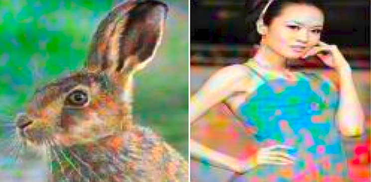
Succesful fully automatic approaches emerged only recently [Iizuka et al.(2016)Iizuka, Simo-Serra, and Ishikawa, Larsson et al.(2016)Larsson, Maire, and Shakhnarovich, Zhang et al.(2016)Zhang, Isola, and Efros, Isola et al.(2016)Isola, Zhu, Zhou, and Efros, Deshpande et al.(2016)Deshpande, Lu, Yeh, and Forsyth, Cao et al.(2017)Cao, Zhou, Zhang, and Yu] based on deep architectures. A straight-forward approach is to train a convolutional feedforward model to independently predict a color value for each pixel [Iizuka et al.(2016)Iizuka, Simo-Serra, and Ishikawa, Larsson et al.(2016)Larsson, Maire, and Shakhnarovich, Zhang et al.(2016)Zhang, Isola, and Efros]. However, these techniques do not model crucial interactions between pixel colors of natural images, and thus, probabilistic sampling yields high-frequency patterns of low perceptual quality (see Figure 1). Predicting the mode or expectation of the learned distribution instead results in grayish, and still often noisy colorizations (see, e.g, Figure 6). Recent unpublished work [Isola et al.(2016)Isola, Zhu, Zhou, and Efros] proposes to train colorization model using generative adversarial networks (GANs) [Goodfellow et al.(2014)Goodfellow, Pouget-Abadie, Mirza, Xu, Warde-Farley, Ozair, Courville, and Bengio]. GANs, however, are known to suffer from unstable training and lack of a consistent objective, which often prevents a quantitative comparison of models.

A shared limitation of the models discussed above is their lack of diversity. They can only produce one colored version from each grayscale image, despite the fact that are typically multiple plausible colorizations. [Cao et al.(2017)Cao, Zhou, Zhang, and Yu] for instance addresses the problem in the framework of conditional GANs. To our knowledge, the only work besides ours aiming at representing a fully probabilistic multi-modal joint distribution of pixel colors is [Deshpande et al.(2016)Deshpande, Lu, Yeh, and Forsyth]. It relies on the variational autoencoder framework [Kingma and Welling(2014)], which, however, tends to produce more blurry outputs than other image generating techniques. In contrast, the autoregressive [van den Oord et al.(2016b)van den Oord, Kalchbrenner, and Kavukcuoglu, Salimans et al.(2017)Salimans, Karpathy, Chen, Knigma, and Bulatov] network that we employ is able to produce crisp high-quality and diverse colorizations.

3 Probabilistic Image Colorization

In this section we present our Probabilistic Image Colorization model (PIC). We first introduce the technical background, then formulate the proposed probabilistic model and conclude with parametrization and optimization details.

3.1 Background

Let $X$ be a natural image containing $n$ pixels, indexed in raster scan order: from top to bottom and from left to right; the value of the $i$-th pixel is denoted as $X_{i}$. We assume that images are encoded in the LAB color space, which has three channels: the luminance channel (L) and the two chrominance channels (a and b). We denote by $X^{L}$ and $X^{ab}$ the projection of $X$ to its luminance channel and chrominance channels respectively. By convention a Lab triplet belongs to the range $[0;100]\times[-127;128]\times[-128;127]$. Consequently, each pixel in $X^{ab}$ can take $256\times 256=65536$ possible values.

Our goal is to predict a probabilistic distribution of image colors from an input gray image (luminance channel), i.ewe model the conditional distribution $p(X^{ab}|X^{L})$ from a set of training images, $\mathcal{D}$. This is a challenging task, as $X^{ab}$ is a high dimensional object with a rich internal structure.

3.2 Modeling the joint distribution of image colors

To tackle the aforementioned task we rely on recent advances in autoregressive probabilistic models [van den Oord et al.(2016b)van den Oord, Kalchbrenner, and Kavukcuoglu, Salimans et al.(2017)Salimans, Karpathy, Chen, Knigma, and Bulatov]. The main insight is to use the chain rule in order to decompose the distribution of interest into elementary per-pixel conditional distributions; all of these distributions are modeled using a shared deep convolutional neural network:

$$p(X^{ab}|X^{L})=\prod_{i=1}^{n}p(X_{i}^{ab}|X_{i-1}^{ab},\dots,X_{1}^{ab};\ X^{L}).$$ (1)

Note, that (1) makes no assumptions on the modeled distribution. It is only an application of the chain rule of probability theory. At training time, all variables in the factors are observed, so a model can be efficiently trained by learning all factors in parallel. At test time, we can draw a sample from the joint distribution using a pixel-level sequential procedure: we first sample $X_{1}^{ab}$ from $p(X_{1}^{ab}|X^{L})$, then sample $X_{i}^{ab}$ from $p(X_{i}^{ab}|X_{i-1}^{ab},\dots X_{1}^{ab};X^{L})$ for all $i$ in $\{2\dots n\}$.

We denote the deep autoregressive neural network for modeling factors from (1) as $f^{\theta}$, where $\theta$ is a vector of parameters. The autoregressive network $f^{\theta}$ outputs a vector of normalized probabilities over the set, $\mathcal{C}$, of all possible chrominance (a, b) pairs. For brevity, we denote a predicted probability for the pixel value $X_{i}^{ab}$ as $f^{\theta}_{i}$. To model the dependency on the observed grayscale image view $X^{L}$ we additionally introduce a deep neural network $g^{w}(X^{L})$, which produces a suitable embedding of $X^{L}$. To summarize, formally, each factor in (1) has the following functional form:

$$p(X_{i}^{ab}|X_{i-1}^{ab},\dots,X_{1}^{ab};\ X^{L})=f^{\theta}_{i}(X_{i-1}^{ab},\dots,X_{1}^{ab};\ g^{w}(X^{L}))$$ (2)

Note, that the autoregressive network $f^{\theta}$ outputs a probability distribution over all color values in $\mathcal{C}$. The standard way to encode such a distribution over discrete values is to parametrize $f^{\theta}$ to output a score for each of the possible color values in $\mathcal{C}$ and then apply the softmax operation to obtain a normalized distribution. In our case, however, the output space is huge (65536 values per pixel), and the standard approach has crucial shortcomings: it will result in a very slow convergence of the training procedure and will require a vast amount of data to generalize. It is possible to alleviate this shortcoming by quantizing the colorspace at the expense of a slight drop in colorization accuracy and possible visible quantization artifacts. Furthermore, it still results in a large number of classes, typically a few hundreds, leading to slow convergence; additional heuristics, such as soft label encoding [Zhang et al.(2016)Zhang, Isola, and Efros], are then required to speed up the training.

Instead, we approximate the distribution in (2) with a mixture of $10$ logistic distributions, as described in [Salimans et al.(2017)Salimans, Karpathy, Chen, Knigma, and Bulatov]. This requires $f^{\theta}$ to output the mixture weights as well as the first and second-order statistics of each mixture. In practice, we need less than 100 output values per pixel to encode those, which is significantly fewer than for the standard discrete distribution representation. This model is powerful enough to represent a multimodal discrete distribution over all values in $\mathcal{C}$. Furthermore, since the representation is partially continuous, it can make use of the distance of the color values in the real space, resulting in faster convergence.

In the rest of the section section we give details on the architecture for $g^{w}$ and $f^{\theta}$ and on the optimization procedure.

Figure 2: High-level scheme for the proposed model.

3.3 Model architecture and training procedure

We present a high-level overview of our model in Figure 2. It has two major components: the embedding network $g^{w}$ and the autoregressive network $f^{\theta}$. Intuitively, we expect that $g^{w}$, which only has access to the grayscale input, produces an embedding encoding information about plausible image colors based on the semantics available in the grayscale image. The autoregressive network then makes use of this embedding to produce the final colorization, while being able to model complex interactions between image pixels.

Our design choices for parametrizing networks $g^{w}$ and $f^{\theta}$ are motivated by [Salimans et al.(2017)Salimans, Karpathy, Chen, Knigma, and Bulatov], as it reports state-of-the-art results for the challenging and related problem of natural image modeling. In particular, we use gated residual blocks as the main building component for the both networks. Each residual block has 2 convolutions with 3x3 kernels, a skip connection [He et al.(2016)He, Zhang, Ren, and Sun] and gating mechanism [van den Oord et al.(2016a)van den Oord, Kalchbrenner, Espeholt, Vinyals, and Graves, Salimans et al.(2017)Salimans, Karpathy, Chen, Knigma, and Bulatov]. Convolutions are preceded by concatenated [Shang et al.(2016)Shang, Sohn, Almeida, and Lee] exponential linear units [Clevert et al.(2016)Clevert, Unterthiner, and Hochreiter] as non-linearities and parametrized as proposed in [Salimans and Kingma(2016)]. If specified, the first convolution of the residual block may have a dilated receptive field [Yu and Koltun(2016)]; we use dilation to increase the network’s field-of-view without reducing its spatial resolution.

The embedding network $g^{w}$ is a standard feed-forward deep convolutional neural network. It consist of gated residual blocks and (strided) convolutions. We give more precise details on the architecture in the experimental section.

For parametrizing $f^{\theta}$ we use the PixelCNN++ architecture from [Salimans et al.(2017)Salimans, Karpathy, Chen, Knigma, and Bulatov]. On a high level, the network consists of two flows of residual blocks, where the output of every convolution is properly shifted to achieve sequential dependency: $X_{i}^{ab}$ depends only on $X_{i-1}^{ab},\dots,X_{1}^{ab}$. Conditioning on the external input, $X^{L}$, is achieved by biasing the output of the first convolution of every residual block by the embedding $g^{w}(X^{L})$. We use no down- or up-sampling layers. For more detailed explanation of this architecture see our implementation or [Salimans et al.(2017)Salimans, Karpathy, Chen, Knigma, and Bulatov].

Spatial chromatic subsampling.

It is known that the human visual system resolves color less precisely than luminance information [Van der Horst and Bouman(1969)]. We exploit this fact by modeling the chrominance channels at a lower resolution than the input luminance. This allows us to reduce computational and memory requirements without losing perceptual quality. Note that image compression schemes such as JPEG or previously proposed techniques for automatic colorization also make use of chromatic subsampling.

Optimization.

We train the parameters $\theta$ and $w$ by minimizing the negative log-likelihood of the chrominance channels in the training data:

$$\arg\min\limits_{\theta,w}\sum_{X\in\mathcal{D}}-\log p(X^{ab}|X^{L})$$ (3)

We use the Adam optimizer [Kingma and Ba(2014)] with an initial learning rate of 0.001, momentum of 0.95 and second momentum of 0.9995. We also apply Polyak parameter averaging [Polyak and Juditsky(1992)].

CIFAR-10 embedding $g^{w}(X^{L})$
Operation	Res.	Width	D
Conv. 3x3/1	32	32	–
Resid. block $\times$ 2	32	32	–
Conv. 3x3/2	16	64	–
Resid. block $\times$ 2	16	64	–
Conv. 3x3/1	16	128	–
Resid. block $\times$ 2	16	128	–
Conv. 3x3/1	16	256	–
Resid. block $\times$ 3	16	256	2
Conv. 3x3/1	16	256	–

ILSVRC 2012 embedding $g^{w}(X^{L})$
Operation	Res.	Width	D
Conv. 3x3/1	128	64	–
Resid. block $\times$ 2	128	64	–
Conv. 3x3/2	64	128	–
Resid. block $\times$ 2	64	128	–
Conv. 3x3/2	32	256	–
Resid. block $\times$ 2	32	256	–
Conv. 3x3/1	32	512	–
Resid. block $\times$ 3	32	512	2
Conv. 3x3/1	32	512	–
Resid. block $\times$ 3	32	512	4
Conv. 3x3/1	32	512	–

Table 1: Architecture of $g^{w}$ for the CIFAR-10 and ILSVRC 2012 datasets. The notation “$\times\ k$” in the Operation column means the corresponding operation is repeated $k$ times. Res. is the layer’s spatial resolution, Width is the number of channels and D is the dilation rate.

4 Experiments

In this section we present quantitative and qualitative evaluation of the proposed probabilistic image colorization (PIC) technique. We evaluate our model on two challenging image datasets: CIFAR-10 and ImageNet ILSVRC 2012. We also qualitatively compare our method to previously proposed colorization approaches and perform additional studies to better understand various components of our model. We will make our Tensorflow implementation publicly available soon.

4.1 CIFAR-10 experiments

We first study the colorization abilities of our method on the CIFAR-10 dataset, which contains 50000 training images and 10000 test images of 32x32 pixels, categorized in 10 semantic classes. We fix the architecture of the embedding network $g^{w}$ as specified in Table 1 (left). For the autoregressive network $f^{\theta}$ we use 4 residual blocks and 160 output channels for every convolution. We subsample the spatial chromatic resolution by a factor of 2, i.emodel the color channels on the resolution of 16x16. We train the resulting model as explained in Section 3 with batch size of 64 images for 150 epochs. The learning rate decays after every training iteration with constant multiplicative rate 0.99995.

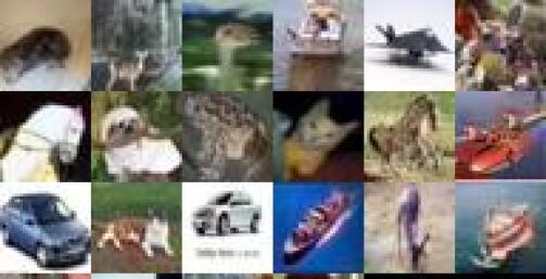
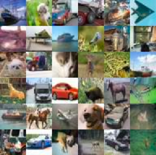
In Figure 3 we visualize random test images colorized by PIC (left) and the corresponding real CIFAR-10 color images (right). We note that the samples produced by PIC appear to have natural colors and are hardly distinguishable from the real ones. This speaks in favour of our model being appropriate for modeling the color distribution of natural images.

We also report that PIC achieves a negative log-likelihood of 2.72, measured in bits-per-dimension. Intuitively, this measure indicates the average amount of uncertainty in the image colors under the trained model. This is a principled measure that can be used to perform model selection and compare various probabilistic colorization techniques.

4.2 ILSVRC 2012 experiments

After preliminary experiments on the CIFAR-10 dataset we now present experimental evaluation of PIC on the much more challenging ILSVRC 2012. This dataset has 1.2 million high-resolution training images spread over 1000 different semantic categories, and a hold-out set of 50000 validation images. In our experiments we rescale all images to 128x128 pixels, which is enough to capture essential image details and remain a challenging scenario. Note, however, that in principle our method is applicable and scales to higher resolutions.

As ILSVRC images are of higher resolution and contain more details than CIFAR-10 images, we use a slightly bigger architecture for the embedding function $g^{w}$ as specified in Table 1 (right) and a chroma subsampling factor of 4, as in [Zhang et al.(2016)Zhang, Isola, and Efros]. The autoregressive component $f^{\theta}$ has 4 residual blocks and 160 channels for every convolution.

Figure 3: Colorized image samples from our model (left) and the corresponding original CIFAR-10 images (right). Images are selected randomly from the test set.

We run the optimization algorithm for 20 epochs using batches of 64 images, with learning rate decaying multiplicatively after every iteration with the constant of 0.99999.

In Figure 4 we present successfully colorized images from the validation set. These demonstrate that our model is capable of producing spatially coherent and semantically plausible colors. Moreover, as expected, in the case where the color is ambiguous, the produced samples often demonstrate wide color diversity. Nevertheless, if the color is mostly determined by the semantics of the object (grass or sky), then PIC produces consistent colors.

To provide further insight, we also highlight two failure cases in Figure 5: First, PIC may not fully capture complex long-range pixel interactions interactions, e.g, if an object is split due to occlusion, the two parts may have different colors. Second, for some complex images with unusual objects PIC may fail to understand semantics of the image and produce not visually plausible colors.

Our model achieves a negative log-likelihood of 2.51 bits-per-dimension. Note that purely generative model from [van den Oord et al.(2016b)van den Oord, Kalchbrenner, and Kavukcuoglu], which is based on the similar but deeper architecture, reports a negative log-likehood of 3.86 for the ILSVRC validation images modeled on the same resolution. As our model has access to additional information (grayscale input), it is not surprising that we achieve better likelihood; Nevertheless, this result confirms that PIC learns non-trivial colorization model and strengthens our qualitative evaluation.

 

Figure 4: Colorized samples from our model illustrate its ability to produce diverse (top) or consistent (bottom) samples depending whether the image semantics are ambiguous or not.

4.3 Importance of the autoregressive component

One of the main novelties of our model is the autoregressive component, $f^{\theta}$, which drastically increases the colorization performance by modeling the joint distribution over all pixels. In this section we perform an ablation study in order to investigate the importance of the autoregressive component alone. Note that without $f^{\theta}$, our model essentially becomes a standard feed-forward neural network, similar to recent colorization techniques [Zhang et al.(2016)Zhang, Isola, and Efros, Larsson et al.(2016)Larsson, Maire, and Shakhnarovich], Specifically, we use PIC pretrained on the ILSVRC dataset, discard the autoregressive component $f^{\theta}$, and finetune the remaining embedding network, $g^{w}$, for the task of image colorization. At test time, we use maximum a posteriori (MAP) sampling from this model. Stochastic sampling from the output of $g^{w}$ would produce very noisy colorizations as the pixelwise predicted distributions are independent. Alternatively, one could predict the mean color of the predicted distribution for each pixel, but that would produce mostly gray colors.

Figure 5: Illustration of failure cases: PIC may fail to reflect very long-range pixel interactions (top) and, e.g, assign different colors to disconnected parts of an occluded object, or it may fail to understand semantics of complex scenes with unusual objects (bottom).

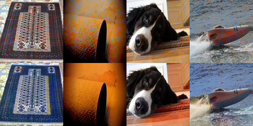
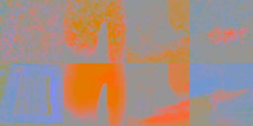
From comparing the output samples of PIC and $g^{w}$, it appears the benefit brought by the autoregressive component is two-fold: first, it explicitly models relationships between neighboring pixels, which leads to visually smoother samples as can be seen in Figure 6. Second, the samples generated from PIC tend to display more saturated colors. This is due to the fact that our model allows for proper probabilistic sampling and, thus, can produce rare and globally consistent colors. We also verify that PIC produces more vivid colors by computing the average perceptual saturation [Lübbe(2010)]. Based on 1000 random image samples, the PIC model and $g^{w}$ have an average saturation of 36.4% and 32.7%, respectively.

Figure 6: Comparison on ImageNet validation set between MAP samples from the embedding network $g_{w}$ (top) and random samples from the autoregressive PIC model (bottom). Colored image (left) and predicted chrominances for fixed $\mathbf{L}=50$ (right)

4.4 Model selection and gating non-linearity

Figure 7: Comparison of CIFAR-10 colorization samples obtained without gating (left) and with gating (right).

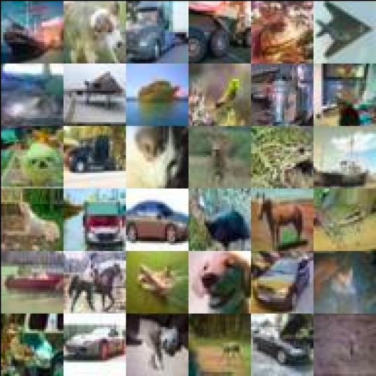
Recently it was demonstrated that gating non-linearity is useful for the task of natural image modeling [van den Oord et al.(2016b)van den Oord, Kalchbrenner, and Kavukcuoglu]. Thus, we expect that gating should be also beneficial for colorization, which is closely related to image modeling.

One way to verify whether gating is useful is to perform qualitative sample analysis. We illustrate samples from the PIC model, as well as the samples from the identical model without gating non-linearity in Figure 7. We observe that even though the samples obtained with the gating mechanism appear to have higher visual quality, i.ehave slightly more saturated colors and better global consistency, it is hard to make definitive conclusion.

Thus, we also perform quantitative analysis using the likelihood measure. PIC with gating achieves the negative log-likelihood of 2.72, while its counterpart without gating achieves 2.78. The quantitative evaluation is consistent with our preliminary qualitative evaluation.

We argue that the negative log-likelihood on the hold-out image set may be used as a principled measure for model selection. Importantly, our metric measures how well the joint distribution of image colors is explained by the model. Unlike all previous metrics, which were used to evaluate image colorization performance, our metric accounts for intrinsic uncertainty of the task and, at the same time, for modeling complex interactions between pixels within one image.

4.5 Qualitative comparison to baselines.

In Figure 4.5 we present a few colorization results on the ImageNet validation set for our model (one sample) as well as three recent colorization baselines. Zhang et al., 2016 [Zhang et al.(2016)Zhang, Isola, and Efros] proposes a deep VGG architecture trained on ImageNet for automatic colorization. The main innovation is that they treat colorization as a classification rather than regression task, combined with class-rebalancing in the training loss to favor rare colors and more vibrant samples. Larsson et al., 2016 [Larsson et al.(2016)Larsson, Maire, and Shakhnarovich] is very similar to the first baseline, except for a few architectural differences (e.g, use of hypercolumns) and heuristics. Iizuka et al., 2016 [Iizuka et al.(2016)Iizuka, Simo-Serra, and Ishikawa] proposes a non-probabilistic model with a regression objective. Their architecture is also more complex as as they use two distinct flows for local and global features. We also note that their model was trained on the MIT Places dataset, while ours and the two previous baselines use ImageNet. We use the publicly available implementation for each baseline.

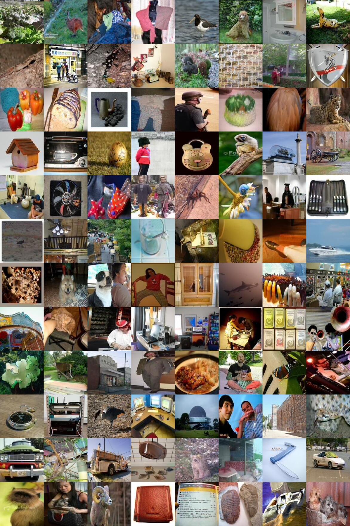
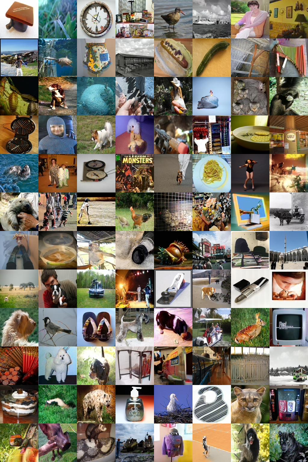
In general, we observe that our model is highly competitive with other approaches and tends to produce more saturated colors on average. We will also include more samples from our model in the appendix, see Figures 9 and 10.

Input	[Zhang et al.]	[Larsson et al.]	[Iizuka et al.]	Ours	Original
* #1 in 3

* #1 in 1 2 3 5 &

Figure 8: Qualitative results from several recent automatic colorization methods compared to the original (right) and sample from our method (first to last column).

5 Conclusion

Deep feedforward networks achieve promising results on the task of colorizing natural gray images. The generated samples however often suffer of a lack of diversity and color vibrancy. We tackle both aspects by modelling the full joint distribution of pixel color values using an autoregressive network conditioned on a learned embedding of the grayscale image. The fully probabilistic nature of this framework provides us with a proper and straightforward sampling mechanism, hence the ability to generate diverse samples from a given grayscale input. Furthermore, the data likelihood can be efficiently computed from the model and used as a quantitative evaluation metric. We report quantitative and qualitative evaluations of our model, and show that colorizations sampled from our architecture often display vivid colors, indicating that the model captures well the underlying color distribution of natural images, without requiring any ad hoc heuristics during training.

6 Appendix

Figure 9: Random colorized images from the ILSVRC 2012 validation set (part 1).

Figure 10: Random colorized images from the ILSVRC 2012 validation set (part2).

References

- [Cao et al.(2017)Cao, Zhou, Zhang, and Yu] Yun Cao, Zhiming Zhou, Weinan Zhang, and Yong Yu. Unsupervised diverse colorization via generative adversarial networks. arXiv preprint arXiv:1702.06674, 2017.
- [Charpiat et al.(2008)Charpiat, Hofmann, and Schölkopf] Guillaume Charpiat, Matthias Hofmann, and Bernhardt Schölkopf. Automatic image colorization via multimodal predictions. In European Conference on Computer Vision (ECCV), 2008.
- [Clevert et al.(2016)Clevert, Unterthiner, and Hochreiter] Djork-Arné Clevert, Thomas Unterthiner, and Sepp Hochreiter. Fast and accurate deep network learning by exponential linear units (ELUs). In International Conference on Learning Representations (ICLR), 2016.
- [Deshpande et al.(2015)Deshpande, Rock, and Forsyth] Aditya Deshpande, Jason Rock, and David A. Forsyth. Learning large-scale automatic image colorization. In International Conference on Computer Vision (ICCV), 2015.
- [Deshpande et al.(2016)Deshpande, Lu, Yeh, and Forsyth] Aditya Deshpande, Jiajun Lu, Mao-Chuang Yeh, and David A. Forsyth. Learning diverse image colorization. arXiv preprint arXiv:1612.01958, 2016.
- [Goodfellow et al.(2014)Goodfellow, Pouget-Abadie, Mirza, Xu, Warde-Farley, Ozair, Courville, and Bengio] Ian Goodfellow, Jean Pouget-Abadie, Mehdi Mirza, Bing Xu, David Warde-Farley, Sherjil Ozair, Aaron Courville, and Yoshua Bengio. Generative adversarial networks. In Conference on Neural Information Processing Systems (NIPS), 2014.
- [He et al.(2016)He, Zhang, Ren, and Sun] Kaiming He, Xiangyu Zhang, Shaoqing Ren, and Jian Sun. Deep residual learning for image recognition. In Conference on Computer Vision and Pattern Recognition (CVPR), 2016.
- [Iizuka et al.(2016)Iizuka, Simo-Serra, and Ishikawa] Satoshi Iizuka, Edgar Simo-Serra, and Hiroshi Ishikawa. Let there be color!: Joint end-to-end learning of global and local image priors for automatic image colorization with simultaneous classification. ACM Transactions on Graphics (Proceedings of SIGGRAPH), 2016.
- [Isola et al.(2016)Isola, Zhu, Zhou, and Efros] Phillip Isola, Jun-Yan Zhu, Tinghui Zhou, and Alexei A. Efros. Image-to-image translation with conditional adversarial networks. arXiv preprint arXiv:1611.07004, 2016.
- [Kingma and Ba(2014)] Diederik P. Kingma and Jimmy Ba. Adam: A method for stochastic optimization. CoRR, abs/1412.6980, 2014.
- [Kingma and Welling(2014)] Diederik P Kingma and Max Welling. Auto-encoding variational bayes. In International Conference on Learning Representations (ICLR), 2014.
- [Kingma et al.(2016)Kingma, Salimans, and Welling] Diederik P. Kingma, Tim Salimans, and Max Welling. Improving variational inference with inverse autoregressive flow. In Conference on Neural Information Processing Systems (NIPS), 2016.
- [Larsson et al.(2016)Larsson, Maire, and Shakhnarovich] Gustav Larsson, Michael Maire, and Gregory Shakhnarovich. Learning representations for automatic colorization. In European Conference on Computer Vision (ECCV), 2016.
- [Levin et al.(2004)Levin, Lischinski, and Weiss] Anat Levin, Dani Lischinski, and Yair Weiss. Colorization using optimization. ACM Transactions on Graphics (Proceedings of SIGGRAPH), 2004.
- [Lübbe(2010)] E. Lübbe. Colours in the Mind - Colour Systems in Reality: A formula for colour saturation. Books on Demand, 2010.
- [Markle and Hunt(1988)] Wilson Markle and Brian Hunt. Coloring a black and white signal using motion detection, 1988. US Patent 4,755,870.
- [Morimoto et al.(2009)Morimoto, Taguchi, and Naemura] Yuji Morimoto, Yuichi Taguchi, and Takeshi Naemura. Automatic colorization of grayscale images using multiple images on the web. ACM Transactions on Graphics (Proceedings of SIGGRAPH), 2009.
- [Novak(1972)] Joseph F. Novak. Method and apparatus for converting monochrome pictures to multi-color pictures electronically, 1972. US Patent 3,706,841.
- [Polyak and Juditsky(1992)] Boris T Polyak and Anatoli B Juditsky. Acceleration of stochastic approximation by averaging. SIAM Journal on Control and Optimization, 1992.
- [Salimans and Kingma(2016)] Tim Salimans and Diederik P Kingma. Weight normalization: A simple reparameterization to accelerate training of deep neural networks. In Conference on Neural Information Processing Systems (NIPS), 2016.
- [Salimans et al.(2017)Salimans, Karpathy, Chen, Knigma, and Bulatov] Tim Salimans, Andrej Karpathy, Xi Chen, Diederik P. Knigma, and Yaroslav Bulatov. PixelCNN++: A PixelCNN implementation with discretized logistic mixture likelihood and other modifications. In International Conference on Learning Representations (ICLR), 2017.
- [Shang et al.(2016)Shang, Sohn, Almeida, and Lee] Wenling Shang, Kihyuk Sohn, Diogo Almeida, and Honglak Lee. Understanding and improving convolutional neural networks via concatenated rectified linear units. In International Conference on Machine Learing (ICML), 2016.
- [van den Oord et al.(2016a)van den Oord, Kalchbrenner, Espeholt, Vinyals, and Graves] Aaron van den Oord, Nal Kalchbrenner, Lasse Espeholt, Oriol Vinyals, and Alex Graves. Conditional image generation with pixelCNN decoders. In Conference on Neural Information Processing Systems (NIPS), 2016a.
- [van den Oord et al.(2016b)van den Oord, Kalchbrenner, and Kavukcuoglu] Aaron van den Oord, Nal Kalchbrenner, and Koray Kavukcuoglu. Pixel recurrent neural networks. In International Conference on Machine Learing (ICML), 2016b.
- [Van der Horst and Bouman(1969)] Gerard JC Van der Horst and Maarten A Bouman. Spatiotemporal chromaticity discrimination. Journal of the Optical Society of America (JOSA), 59(11):1482–1488, 1969.
- [Yu and Koltun(2016)] Fisher Yu and Vladlen Koltun. Multi-scale context aggregation by dilated convolutions. In International Conference on Learning Representations (ICLR), 2016.
- [Zhang et al.(2016)Zhang, Isola, and Efros] Richard Zhang, Phillip Isola, and Alexei A Efros. Colorful image colorization. In European Conference on Computer Vision (ECCV), 2016.