Distributionally Robust Groupwise Regularization Estimator

Abstract.

Regularized estimators in the context of group variables have been applied successfully in model and feature selection in order to preserve interpretability. We formulate a Distributionally Robust Optimization (DRO) problem which recovers popular estimators, such as Group Square Root Lasso (GSRL). Our DRO formulation allows us to interpret GSRL as a game, in which we learn a regression parameter while an adversary chooses a perturbation of the data. We wish to pick the parameter to minimize the expected loss under any plausible model chosen by the adversary - who, on the other hand, wishes to increase the expected loss. The regularization parameter turns out to be precisely determined by the amount of perturbation on the training data allowed by the adversary. In this paper, we introduce a data-driven (statistical) criterion for the optimal choice of regularization, which we evaluate asymptotically, in closed form, as the size of the training set increases. Our easy-to-evaluate regularization formula is compared against cross-validation, showing good (sometimes superior) performance.

1. Introduction

Group Lasso (GR-Lasso) estimator is a generalization of the Lasso estimator (see Tibshirani, (1996)). The method focuses on variable selection in settings where some predictive variables, if selected, must be chosen as a group. For example, in the context of the use of dummy variables to encode a categorical predictor, the application of the standard Lasso procedure might result in the algorithm including only a few of the variables but not all of them, which could make the resulting model difficult to interpret. Another example, where the GR-Lasso estimator is particularly useful, arises in the context of feature selection. Once again, a particular feature might be represented by several variables, which often should be considered as a group in the variable selection process.
The GR-Lasso estimator was initially developed for the linear regression case (see Yuan and Lin, (2006)), but a similar group-wise regularization was also applied to logistic regression in Meier et al., (2008). A brief summary of GR-Lasso technique type of methods can be found in Friedman et al., (2010).
Recently, Bunea et al., (2014) developed a variation of the GR-Lasso estimator, called the Group-Square-Root-Lasso (GSRL) estimator, which is very similar to the GR-Lasso estimator. The GSRL is to the GR-Lasso estimator what sqrt-Lasso, introduced in Belloni et al., (2011), is to the standard Lasso estimator. In particular, GSRL has a superior advantage over GR-Lasso, namely, that the regularization parameter can be chosen independently from the standard deviation of the regression error in order to guarantee the statistical consistency of the regression estimator (see Belloni et al., (2011), and Bunea et al., (2014)).

Our contribution in this paper is to provide a DRO representation for the GSRL estimator, which is rich in interpretability and which provides insights to optimally select (using a natural criterion) the regularization parameter without the need of time-consuming cross-validation. We compute the optimal regularization choice (based on a simple formula we derive in this paper) and evaluate its performance empirically. We will show that our method for the regularization parameter is comparable, and sometimes superior, to cross-validation.

In order to describe our contributions more precisely, let us briefly describe the GSRL estimator. We choose the context of linear regression to simplify the exposition, but an entirely analogous discussion applies to the context of logistic regression.
Consider a given a set of training data $\{(X_{1},Y_{1}),\ldots,(X_{n},Y_{n})\}$. The input $X_{i}\in\mathbb{R}^{d}$ is a vector of $d$ predicting variables, and $Y_{i}\in\mathbb{R}$ is the response variable. (Throughout the paper any vector is understood to be a column vector and the transpose of $x$ is denoted by $x^{T}$.) We use $\left(X,Y\right)$ to denote a generic sample from the training data set. It is postulated that

$$Y_{i}=X_{i}^{T}\beta^{\ast}+e_{i},$$

for some $\beta^{\ast}\in\mathbb{R}^{d}$ and errors $\left\{e_{1},...,e_{n}\right\}$. Under suitable statistical assumptions (such as independence of the samples in the training data), one may be interested in estimating $\beta^{\ast}$.
Underlying, we consider the square loss function, i.e. $l\left(x,y;\beta\right)=\left(y-\beta^{T}x\right)^{2}$, for the purpose of this discussion but this choice, as we shall see, is not necessary.

Throughout the paper we will assume the following group structure for the space of predictors. There are $\bar{d}\leq d$ mutually exclusive groups, which form a partition. More precisely, suppose that $G_{1},\ldots,G_{\bar{d}}$ satisfies that $G_{i}\cap G_{j}=\varnothing$ for $i\neq j$, that $G_{1}\cup...\cup G_{\bar{d}}=\{1,...,d\}$, and the $G_{i}$’s are non-empty. We will use $g_{i}$ to denote the cardinality of $G_{i}$ and shall write $G$ for a generic set in the partition and let $g$ denote the cardinality of $G$.
We shall denote by $x\left(G\right)\in\mathbb{R}^{g}$ the sub-vector $x\in\mathbb{R}^{d}$ corresponding to $G$. So, if $G=\{i_{1},...,i_{g}\}$, then $x\left(G\right)=\left(X_{i_{1}},\ldots,X_{i_{g}}\right)^{T}$.
Next, given $p,s\geq 1$, and $\alpha\in\mathbb{R}_{++}^{\bar{d}}$ (i.e. $\alpha_{i}>0$ for $1\leq i\leq\bar{d}$) we define for each $x\in\mathbb{R}^{d}$,

(1) $$\left\|x\right\|_{\alpha\text{-}(p,s)}=\left(\sum_{i=1}^{\bar{d}}\alpha_{i}^{s}\left\|x\left(G_{i}\right)\right\|_{p}^{s}\right)^{1/s},$$

where $\left\|x\left(G_{i}\right)\right\|_{p}$ denotes the $p$-norm of $x\left(G_{i}\right)$ in $\mathbb{R}^{g_{i}}$. (We will study fundamental properties of $\left\|x\right\|_{\alpha\text{-}(p,s)}$ as a norm in Proposition 1.)
Let $P_{n}$ be the empirical distribution function, namely,

$$P_{n}\left(dx,dy\right):=\frac{1}{n}\sum_{i=1}^{n}\mathcal{\delta}_{\left\{(X_{i},Y_{i})\right\}}(dx,dy).$$

Throughout out the paper we use the notation $\mathbb{E}_{P}[\cdot]$ to denote expectation with respect to a probability distribution $P$.
The GSRL estimator takes the form

$$\min_{\beta}\sqrt{\frac{1}{n}\sum_{i=1}^{n}l\left(X_{i,}Y_{i};\beta\right)}+\lambda\left\|\beta\right\|_{\tilde{g}^{-1}-\left(2,1\right)}=\min_{\beta}\left(\mathbb{E}_{P_{n}}^{1/2}\left[l\left(X,Y;\beta\right)\right]+\lambda\left\|\beta\right\|_{\sqrt{\tilde{g}}-\left(2,1\right)}\right),$$

where $\lambda$ is the so-called regularization parameter. The previous optimization problem can be easily solved using standard convex optimization techniques as explained in Belloni et al., (2011) and Bunea et al., (2014).

Our contributions in this paper can now be explicitly stated. We introduce a notion of discrepancy, $\mathcal{D}_{c}\left(P,P_{n}\right)$, discussed in Section 2, between $P_{n}$ and any other probability measure $P$, such that

(2) $$\min_{\beta}\max_{P:D_{c}\left(P,P_{n}\right)\leq\delta}\mathbb{E}_{P}^{1/2}\left[l\left(X,Y;\beta\right)\right]=\min_{\beta}\left(\mathbb{E}_{P_{n}}^{1/2}\left[l\left(X,Y;\beta\right)\right]+\delta^{1/2}\left\|\beta\right\|_{\alpha-\left(p,s\right)}\right).$$

Using this representation, which we formulate, together with its logistic regression analogue, in Section 2.2.1 and Section 2.2.2, we are able to draw the following insights:

I) GSRL can be interpreted as a game in which we choose a parameter (i.e. $\beta$) and an adversary chooses a “plausible” perturbation of the data (i.e. $P$); the parameter $\delta$ controls the degree in which $P_{n}$ is allowed to be perturbed to produce $P$. The value of the game is dictated by the expected loss, under $E_{P}$, of the decision variable $\beta$.

II) The set $\mathcal{U}_{\delta}\left(P_{n}\right)=\left\{P:\mathcal{D}_{c}\left(P,P_{n}\right)\leq\delta\right\}$ denotes the set of distributional uncertainty. It represents the set of plausible variations of the underlying probabilistic model which are reasonably consistent with the data.

III) The DRO representation (2) exposes the role of the regularization parameter. In particular, because $\lambda=\delta^{1/2}$, we conclude that $\lambda$ directly controls the size of the distributionally uncertainty and should be interpreted as the parameter which dictates the degree to which perturbations or variations of the available data should be considered.

IV) As a consequence of I) to III), the DRO representation (2) endows the GSRL estimator with desirable generalization properties. The GSRL aims at choosing a parameter, $\beta$, which should perform well for all possible probabilistic descriptions which are plausible given the data.

Naturally, it is important to understand what types of variations or perturbations are measured by the discrepancy $\mathcal{D}_{c}\left(P,P_{n}\right)$. For example, a popular notion of the discrepancy is the Kullback-Leibler (KL) divergence. However, KL divergence has the limitation that only considers probability distributions which are supported precisely on the available training data, and therefore potentially ignores plausible variations of the data which could have an adverse impact on generalization risk.
In the rest of the paper we answer the following questions. First, in Section 2 we explain the nature of the discrepancy $\mathcal{D}_{c}\left(P,P_{n}\right)$, which we choose as an Optimal Transport discrepancy. We will see that $\mathcal{D}_{c}\left(P,P_{n}\right)$ can be computed using a linear program.
Intuitively, $\mathcal{D}_{c}\left(P,P_{n}\right)$ represents the minimal transportation cost for moving the mass encoded by $P_{n}$ into a sinkhole which is represented by $P$. The cost of moving mass from location $u=\left(x,y\right)$ to $w=\left(x^{\prime},y^{\prime}\right)$ is encoded by a cost function $c\left(u,w\right)$ which we shall discuss and this will depend on the $\alpha$-$\left(p,s\right)$ norm that we defined in (1). The subindex $c$ in $\mathcal{D}_{c}\left(P,P_{n}\right)$ represents the dependence on the chosen cost function.
The next item of interest is the choice of $\delta$, again the discussion of items I) to III) of the DRO formulation (2) provides a natural way to optimally choose $\delta$. The idea is that every model $P\in\mathcal{U}_{\delta}\left(P_{n}\right)$ should intuitively represent a plausible variation of $P_{n}$ and therefore $\beta^{P}=\arg\min\left\{\mathbb{E}_{P}[l\left(X,Y;\beta\right)]:\beta\right\}$ is a plausible estimate of $\beta^{\ast}$. The set $\{\beta^{P}:P\in\mathcal{U}_{\delta}\left(P_{n}\right)\}$ therefore yields a confidence region for $\beta^{\ast}$ which is increasing in size as $\delta$ increases. Hence, it is natural to minimize $\delta$ to guarantee a target confidence level (say 95%). In Section 3 we explain how this optimal choice can be asymptotically computed as $n\rightarrow\infty$.
Finally, it is of interest to investigate if the optimal choice of $\delta$ (and thus of $\lambda$) actually performs well in practice. We compare performance of our (asymptotically) optimal choice of $\lambda$ against cross-validation empirically in Section 4. We conclude that our choice is quite comparable to cross validation.

Before we continue with the program that we have outlined, we wish to conclude this Introduction with a brief discussion of work related to the methods discussed in this paper. Connections between regularized estimators and robust optimization formulations have been studied in the literature. For example, the work of Xu et al., (2009) investigates determinist perturbations on the predictor variables to quantify uncertainty. In contrast, our DRO approach quantifies perturbations from the empirical measure. This distinction allows us to statistical theory which is key to optimize the size of the uncertainty, $\delta$ (and thus the regularization parameter) in a data-driven way. The work of Shafieezadeh-Abadeh et al., (2015) provides connections to regularization in the setting of logistic regression in an approximate form. More importantly, Shafieezadeh-Abadeh et al., (2015) propose a data-driven way to choose the size of uncertainty, $\delta$, which is based on the concentration of measure results. The concentration of measure method depends on restrictive assumptions and leads to suboptimal choices, which deteriorate poorly in high dimensions.

The present work is a continuation of the line of research development in Blanchet et al., (2016), which concentrates only on classical regularized estimators without the group structure. Our current contributions require the development of duality results behind the $\alpha$-$\left(p,t\right)$ norm which closely parallels that of the standard duality between $l_{p}$ and $l_{q}$ spaces (with $1/p+1/q=1$) and a number of adaptations and interpretations that are special to the group setting only.

2. Optimal Transport and DRO

2.1. Defining the optimal transport discrepancy

Let $c:\mathbb{R}^{d+1}\times\mathbb{R}^{d+1}\rightarrow[0,\infty]$ be lower semicontinuous and we assume that $c(u,w)=0$ if and only if $u=w$. For reasons that will become apparent in the sequel, we will refer to $c\left(\cdot\right)$ as a cost function.
Given two distributions $P$ and $Q$, with supports $\mathcal{S}_{P}\subseteq\mathbb{R}^{d+1}$ and $\mathcal{S}_{Q}\subseteq\mathbb{R}^{d+1}$, respectively, we define the optimal transport discrepancy, $\mathcal{D}_{c}$, via

(3) $$\mathcal{D}_{c}\left(P,Q\right)=\inf_{\pi}\{E_{\pi}\left[c\left(U,W\right)\right]:\pi\in\mathcal{P}\left(\mathcal{S}_{P}\times\mathcal{S}_{Q}\right),\text{ }\pi_{U}=P,\text{ }\pi_{W}=Q\},$$

where $\mathcal{P}\left(\mathcal{S}_{P}\times\mathcal{S}_{Q}\right)$ is the set of probability distributions $\pi$ supported on $\mathcal{S}_{P}\times\mathcal{S}_{Q}$, and $\pi_{U}$ and $\pi_{W}$ denote the marginals of $U$ and $W$ under $\pi$, respectively.
If, in addition, $c\left(\cdot\right)$ is symmetric (i.e. $c\left(u,w\right)=c\left(w,u\right)$), and there exists $\varrho\geq 1$ such that $c^{1/\varrho}\left(u,w\right)\leq c^{1/\varrho}\left(u,v\right)+c^{1/\varrho}\left(v,w\right)$ (i.e. $c^{1/\varrho}\left(\cdot\right)$ satisfies the triangle inequality), it can be easily verified (see Villani, (2008)) that $\mathcal{D}_{c}^{1/\varrho}\left(P,Q\right)$ is a metric on the probability measures. For example, if $c\left(u,w\right)=\left\|u-w\right\|_{q}^{\varrho}$ for $q\geq 1$ (where $\left\|u-w\right\|_{q}$ denotes the $l_{q}$ norm in $\mathbb{R}^{d+1}$) then $\mathcal{D}_{c}\left(\cdot\right)$ is known as the Wasserstein distance of order $\varrho$.
Observe that (3) is obtained by solving a linear programming problem. For example, suppose that $Q=P_{n}$, so $\mathcal{S}_{P_{n}}=\{\left(X_{i},Y_{i}\right)\}_{i=1}^{n}$, and let $P\$ be supported in some finite set $\mathcal{S}_{P}$ then, using $U=\left(X,Y\right)$, we have that $D_{c}\left(P,P_{n}\right)$ is obtained by computing

(4) $$\left.\min_{\pi}\sum_{u\in\mathcal{S}_{P}}\sum_{w\in\mathcal{S}_{P_{n}}}c\left(u,w\right)\pi\left(u,w\right)\right.$$

s.t. $$\left.\sum_{u\in\mathcal{S}_{P}}\pi\left(u,w\right)=\frac{1}{n}\text{ }\forall\text{ }w\in\mathcal{S}_{P_{n}}\right.$$

$$\left.\sum_{w\in\mathcal{S}_{P_{n}}}\pi\left(u,w\right)=P\left(\left\{u\right\}\right)\text{ }\forall\text{ }u\in\mathcal{S}_{P}\right.$$

$$\left.\pi\left(u,w\right)\geq 0\text{ }\forall\text{ }\left(u,w\right)\in\mathcal{S}_{P}\times\mathcal{S}_{P_{n}}\right..$$

A completely analogous linear program (LP), albeit an infinite dimensional one, can be defined if $\mathcal{S}_{P}$ has infinitely many elements. This LP has been extensively studied in great generality in the context of Optimal Transport under the name of Kantorovich’s problem (see Villani, (2008))).
Note that Kantorovich’s problem is always feasible (take $\pi$ with independent marginals, for example). Moreover, under our assumptions on $c$, if the optimal value is finite, then there is an optimal solution $\pi^{\ast}$ (see Chapter 1 of Villani, (2008))).
It is clear from the formulation of the previous LP that $\mathcal{D}_{c}\left(P,P_{n}\right)$ can be interpreted as the minimal cost of transporting mass from $P_{n}$ to $P$, assuming that the marginal cost of transporting the mass from $u\in\mathcal{S}_{P}$ to $w\in\mathcal{S}_{P_{n}}$ is $c\left(u,w\right)$. It is also not difficult to realize from the assumption that $c\left(u,w\right)=0$ if and only if $u=w$ that $\mathcal{D}_{c}\left(P,P_{n}\right)=0$ if and only if $P=P_{n}$. We shall discuss, for instance, how to choose $c\left(\cdot\right)$ to recover (2) and the corresponding logistic regression formulation of GR-Lasso.

2.2. DRO Representation of GSRL Estimators

In this section, we will construct a cost function $c\left(\cdot\right)$ to obtain the GSRL (or GR-Lasso) estimators. We will follow an approach introduced in Blanchet et al., (2016) for the context of square-root Lasso (SR-Lasso) and regularized logistic regression estimators.

2.2.1. GSRL Estimators for Linear Regression

We start by assuming precisely the linear regression setup described in the Introduction and leading to (2). Given $\alpha=(\alpha_{1},...,\alpha_{\bar{d}})^{T}\in R_{++}^{\bar{d}}$ define $\alpha^{-1}=\left(\alpha_{1}^{-1},...,\alpha_{\bar{d}}^{-1}\right)^{T}$. Now, underlying there is a partition $G_{1},...,G_{\bar{d}}$ of $\{1,...,d\}$ and given $q,t\in[1,\infty]$ we introduce the cost function

(5) $$c\left(\left(x,y\right),\left(x^{\prime},y^{\prime}\right)\right)=\left\{\begin{array}[c]{ccc}\left\|x-x^{\prime}\right\|_{\alpha^{-1}\text{-}(q,t)}^{\varrho}&\text{if}&y=y^{\prime}\\ \infty&\text{if}&y\neq y^{\prime}\end{array}\right.,$$

where, following (1), we have that

$$\left\|x-x^{\prime}\right\|_{\alpha^{-1}\text{-}(q,t)}^{\varrho}=\left(\sum_{i=1}^{\bar{d}}\alpha_{i}^{-t}\left\|x\left(G_{i}\right)-x^{\prime}\left(G_{i}\right)\right\|_{q}^{t}\right)^{\varrho/t}.$$

Then, we obtain the following result.

Theorem 1 (DRO Representation for Linear Regression GSRL).

Suppose that $q,t\in[1,\infty]$ and $\alpha\in R_{++}^{\bar{d}}$ are given and $c\left(\cdot\right)$ is defined as in (5) for $\varrho=2$. Then, if $l\left(x,y;\beta\right)=\left(y-x^{T}\beta\right)^{2}$ we obtain

$$\quad\min_{\beta\in\mathbb{R}^{d}}\sup_{P:D_{c}\left(P,P_{n}\right)\leq\delta}\left(\mathbb{E}_{P}\left[l\left(X,Y;\beta\right)\right]\right)^{1/2}=\min_{\beta\in\mathbb{R}^{d}}\left({E_{P_{n}}\left[l\left(X,Y;\beta\right)\right]}\right)^{1/2}+\sqrt{\delta}\left\|\beta\right\|_{\alpha\text{-}(p,s)},$$

where $1/p+1/q=1$, and $1/s+1/t=1$.

We remark that choosing $p=q=2$, $t=\infty$, $s=1$, and $\alpha_{i}=\sqrt{g_{i}}$ for $i\in\{1,...,\bar{d}\}$ we end up obtaining the GSRL estimator formulated in Bunea et al., (2014)).
We note that the cost function $c\left(\cdot\right)$ only allows mass transportation on the predictors (i.e $X$), but no mass transportation is allowed on the response variable $Y$. This implies that the GSRL estimator implicitly assumes that distributional uncertainty is only present on prediction variables (i.e. variations on the data only occurs through the predictors).

2.2.2. GR-Lasso Estimators for Logistic Regression

We now discuss GR-Lasso for classification problems. We consider a training data set of the form $\{(X_{1},Y_{1}),\ldots,(X_{n},Y_{n})\}$. Once again, the input $X_{i}\in\mathbb{R}^{d}$ is a vector of $d$ predictor variables, but now the response variable $Y_{i}\in\{-1,1\}$ is a categorical variable. In this section we shall consider as our loss function the log-exponential function, namely,

(6) $$l\left(x,y;\beta\right)=\log\left(1+\exp\left(-y\beta^{T}x\right)\right).$$

This loss function is motivated by a logistic regression model which we shall review in the sequel. But for the DRO representation formulation it is not necessary to impose any statistical assumption. We then obtain the following theorem.

Theorem 2 (DRO Representation for Logistic Regression GR-Lasso).

Suppose that $q,t\in[1,\infty]$ and $\alpha\in R_{++}^{\bar{d}}$ are given and $c\left(\cdot\right)$ is defined as in (5) for $\varrho=1$. Then, if $l\left(x,y;\beta\right)$ is defined as in (6) we obtain

$$\min_{\beta\in\mathbb{R}^{d}}\sup_{P:D_{c}\left(P,P_{n}\right)\leq\delta}\mathbb{E}_{P}\left[l\left(X,Y;\beta\right)\right]=\min_{\beta\in\mathbb{R}^{d}}E_{P_{n}}\left(l\left(X,Y;\beta\right)\right)+\delta\left\|\beta\right\|_{\alpha\text{-}(p,s)},$$

where $1\leq q,t\leq\infty$, $1/p+1/q=1$ and $1/s+1/t=1$.

We note that by taking $p=q=2$, $t=\infty$, $s=1$, $\alpha_{i}=\sqrt{g_{i}}$ for $i\in\{1,...,\bar{d}\}$, and $\lambda=\delta$ we recover the GR-Lasso logistic regression estimator from Meier et al., (2008).

As discussed in the previous subsection, the choice of $c\left(\cdot\right)$ implies that the GR-Lasso estimator implicitly assumes that distributionally uncertainty is only present on prediction variables.

3. Optimal Choice of Regularization Parameter

Let us now discuss the mathematical formulation of the optimal criterion that we discussed for choosing $\delta$ (and therefore the regularization parameter $\lambda$). We define

$$\Lambda_{\delta}\left(P_{n}\right)=\{\beta^{P}:P\in\mathcal{U}_{\delta}\left(P_{n}\right)\},$$

as discussed in the Introduction, $\Lambda_{\delta}\left(P_{n}\right)$ is a natural confidence region for $\beta^{\ast}$ because each element $P$ in the distributional uncertainty set $\mathcal{U}_{\delta}\left(P_{n}\right)$ can be interpreted as a plausible variation of the empirical data $P_{n}$. Then, given a confidence level $1-\chi$ (say $1-\chi=.95$) we wish to choose

$$\delta_{n}^{\ast}=\inf\{\delta:P\left(\beta^{\ast}\in\Lambda_{\delta}\left(P_{n}\right)\right)>1-\chi\}.$$

Note that in the evaluation of $P\left(\beta^{\ast}\in\Lambda_{\delta}\left(P_{n}\right)\right)$ the random element is $P_{n}$. So, we shall impose natural probabilistic assumptions on the data generating process in order to asymptotically evaluate $\delta_{n}^{\ast}$ as $n\rightarrow\infty$.

3.1. The Robust Wasserstein Profile Function

In order to asymptotically evaluate $\delta_{n}^{\ast}$ we must recall basic properties of the so-called Robust Wassertein Profile function (RWP function) introduced in Blanchet et al., (2016).
Suppose for each $\left(x,y\right)$, the loss function $l\left(x,y;\cdot\right)$ is convex and differentiable, then under natural moment assumptions which guarantee that expectations are well defined, we have that for

$$P\in\mathcal{U}_{\delta}\left(P_{n}\right)=\{P:D_{c}\left(P,P_{n}\right)\leq\delta\},$$

the parameter $\beta^{P}$ must satisfy

(7) $$\mathbb{E}_{P}\left[\nabla_{\beta}l\left(X,Y;\beta^{P}\right)\right]=0.$$

Now, for any given $\beta$, let us define

$$\mathcal{M}\left(\beta\right)=\left\{P:\mathbb{E}_{P}\left[\nabla_{\beta}l\left(X,Y;\beta\right)\right]=0\right\},$$

which is the set of probability measures $P$, under which $\beta$ is the optimal risk minimization parameter. We would like to choose $\delta$ as small as possible so that

(8) $$\mathcal{U}_{\delta}\left(P_{n}\right)\cap\mathcal{M}\left(\beta^{\ast}\right)\neq\varnothing$$

with probability at least $1-\chi$. But note that (8) holds if and only if there exists $P$ such that $D_{c}\left(P,P_{n}\right)\leq\delta$ and $\mathbb{E}_{P}\left[\nabla_{\beta}l\left(X,Y;\beta^{\ast}\right)\right]=0$.
The RWP function is defined

(9) $$R_{n}\left(\beta\right)=\min\{D_{c}\left(P,P_{n}\right):\mathbb{E}_{P}\left[\nabla_{\beta}l\left(X,Y;\beta\right)\right]=0\}.$$

In view of our discussion following (8), it is immediate that $\beta^{\ast}\in\Lambda_{\delta}\left(P_{n}\right)$ if and only if $R_{n}\left(\beta^{\ast}\right)\leq\delta$, which then implies that

$$\delta_{n}^{\ast}=\inf\{\delta:P\left(R_{n}\left(\beta^{\ast}\right)\leq\delta\right)>1-\chi\}.$$

Consequently, we conclude that $\delta_{n}^{\ast}$ can be evaluated asymptotically in terms of the $1-\chi$ quantile of $R_{n}\left(\beta^{\ast}\right)$ and therefore we must identify the asymptotic distribution of $R_{n}\left(\beta^{\ast}\right)$ as $n\rightarrow\infty$. We illustrate intuitively the role of the RWP function and $\mathcal{M}\left(\beta\right)$ in Figure 1, where RWP function $R_{n}\left(\beta^{\ast}\right)$ could be interpreted as the discrepancy distance between empirical measure $P_{n}$ and the manifold $\mathcal{M}\left(\beta^{\ast}\right)$ associated with $\beta^{\ast}$.

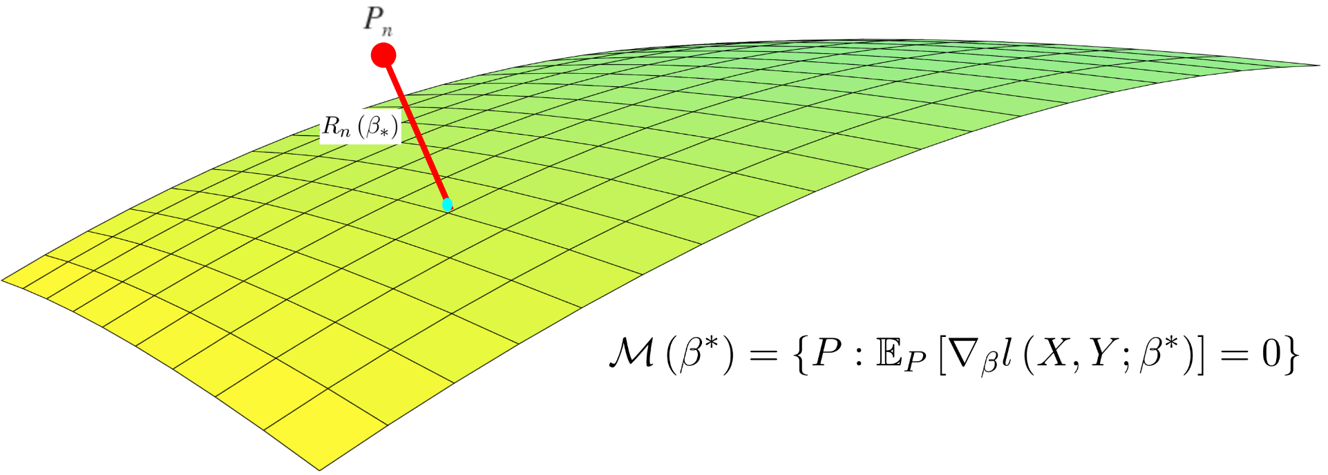
Figure 1. Intuitive Plot for the RWP function $R_{n}\left(\beta\right)$ and the set $\mathcal{M}\left(\beta\right)$.

Typically, under assumptions supporting the underlying model (as in the generalized linear setting we considered), we will have that $\beta^{\ast}$ is characterized by the estimating equation (7). Therefore, under natural statistical assumptions one should expect that $R_{n}\left(\beta^{\ast}\right)\rightarrow 0$ as $n\rightarrow\infty$ at a certain rate and therefore $\delta_{n}^{\ast}\rightarrow 0$ at a certain (optimal) rate. This then yields an optimal rate of convergence to zero for the underlying regularization parameter. The next subsections will investigate the precise rate of convergence analysis of $\delta_{n}^{\ast}$.

3.2. Optimal Regularization for GSRL Linear Regression

We assume, for simplicity, that the training data set $\{(X_{1},Y_{1}),\ldots,(X_{n},Y_{n})\}$ is i.i.d. and that the linear relationship $Y_{i}=\beta^{\ast\;T}X_{i}+e_{i}$, holds with the errors $\left\{e_{1},...,e_{n}\right\}$ being i.i.d. and independent of $\{X_{1},\ldots,X_{n}\}$. Moreover, we assume that both the entries of $X_{i}$ and the errors have finite second moment and the errors have zero mean.
Since in our current setting $l\left(x,y;\beta\right)=\left(y-x^{T}\beta\right)^{2}$, then the RWP function (9) for linear regression model is given as,

(10) $$R_{n}\left(\beta\right)=\min_{P}\left\{D_{c}\left(P,P_{n}\right):\mathbb{E}_{P}\left[X\left(Y-X^{T}\beta\right)\right]=0\right\}.$$

Theorem 3 (RWP Function Asymptotic Results: Linear Regression).

Under the assumptions imposed in this subsection and the cost function as given in (5), with $\varrho=2$,

$$nR_{n}\left(\beta^{\ast}\right)\Rightarrow L_{1}:=\max_{\zeta\in\mathbb{R}^{d}}\left\{2\sigma\zeta^{T}Z-\mathbb{E}\left[\left\|e\zeta-\left(\zeta^{T}X\right)\beta^{\ast}\right\|_{\alpha\text{-}(p,s)}^{2}\right]\right\},$$

as $n\rightarrow\infty$, where $\Rightarrow$ means convergence in distribution and $Z\sim\mathcal{N}\left(0,\Sigma\right)$ with $\Sigma=Var(X)$. Moreover, we can observe the more tractable stochastic upper bound,

$$L_{1}\overset{D}{\leq}L_{2}:=\frac{\mathbb{E}\left[e^{2}\right]}{\mathbb{E}\left[e^{2}\right]-\left(\mathbb{E}\left[\left|e\right|\right]\right)^{2}}\left\|Z\right\|_{\alpha^{-1}\text{-}(q,t)}^{2}.$$

We now explain how to use Theorem 3 to set the regularization parameter in GSRL linear regression:

1. Estimate the $1-\chi$ quantile of $\left\|Z\right\|_{\alpha^{-1}\text{-}(q,t)}^{2}$. We use use $\hat{\eta}_{1-\chi}$ to denote the estimator for this quantile. This step involves estimating $\Sigma$ from the training data.

2. The regularization parameter $\lambda$ in the GSRL linear regression takes the form

   $$\lambda=\sqrt{\delta}=\hat{\eta}_{1-\chi}^{1/2}\left(n(1-\left(\mathbb{E}\left|e\right|\right)^{2}/\mathbb{E}e^{2})\right)^{-1/2}.$$

   Note that the denominator in the previous expression must be estimated from the training data.

Note that the regularization parameter for GSRL for linear regression chosen via our RWPI asymptotic result does not depends on the magnitude of error $e$ (see also the discussion in Bunea et al., (2014)).
It is also possible to formulate the optimal regularization results for high-dimension setting, where the number of predictors growth with sample size. We discuss the results in the Appendix namely Section B.3.

3.3. Optimal Regularization for GR-Lasso Logistic Regression

We assume that the training data set $\{(X_{1},Y_{1}),\ldots,(X_{n},Y_{n})\}$ is i.i.d.. In addition, we assume that the $X_{i}$’s have a finite second moment and also that they possess a density with respect to the Lebesgue measure. Moreover, we assume a logistic regression model; namely,

(11) $$P\left(Y_{i}=1|X_{i}\right)=1/\left(1+\exp\left(-X_{i}^{T}\beta^{\ast}\right)\right),$$

and $P\left(Y_{i}=-1|X_{i}\right)=1-P\left(Y_{i}=1|X_{i}\right)$.
In the logistic regression setting, we consider the log-exponential loss defined in (6). Therefore, the RWP function, (9), for logistic regression is

(12) $$R_{n}\left(\beta\right)=\min\left\{D_{c}\left(P,P_{n}\right):\mathbb{E}_{P}\left[\frac{YX}{1+\exp\left(YX^{T}\beta\right)}\right]=0\right\}.$$

Theorem 4 (RWP Function Asymptotic Results: Logistic Regression).

Under the assumptions imposed in this subsection and the cost function as given in (5) with $\varrho=1$,

$$\sqrt{n}R_{n}\left(\beta^{\ast}\right)\Rightarrow L_{3}:=\sup_{\zeta\in A}\quad\zeta^{T}Z,$$

as $n\rightarrow\infty$, where

$$Z\sim\mathcal{N}\left(0,\mathbb{E}\left[\frac{XX^{T}}{\left(1+\exp\left(YX^{T}\beta^{\ast}\right)\right)^{2}}\right]\right)$$

and

$$A=\left\{\zeta\in\mathbb{R}^{d}:\mathrm{ess}\sup_{X,Y}\left\|\zeta^{T}\frac{y\left(1+\exp\left(YX^{T}\beta^{\ast}\right)\right)I_{d\times d}-XX^{T}}{\left(1+\exp\left(YX^{T}\beta^{\ast}\right)\right)^{2}}\right\|_{\alpha\text{-}(p,s)}\leq 1\right\}.$$

Further, the limit law $L_{3}$ follows the simpler stochastic bound,

$$L_{3}\overset{D}{\leq}L_{4}:=\left\|\tilde{Z}\right\|_{\alpha^{-1}\text{-}(q,t)},$$

where $\tilde{Z}\sim\mathcal{N}\left(0,\Sigma\right)$.

We now explain how to use Theorem 4 to set the regularization parameter in GR-Lasso logistic regression.

1. Estimate the $1-\chi$ quantile of $L_{4}$. We use use $\hat{\eta}_{1-\chi}$ to denote the estimator for this quantile. This step involves estimating $\Sigma$ from the training data.

2. We choose the regularization parameter $\lambda$ in the GR-Lasso problem to be,

   $$\lambda=\delta=\hat{\eta}_{1-\chi}/\sqrt{n}.$$

4. Numerical Experiments

We proceed to numerical experiments on both simulated and real data to verify the performance of our method for choosing the regularization parameter. We apply “grpreg” in R, from Breheny and Breheny, (2016), to solve GR-Lasso for logistic regression. For GSRL for linear regression, we consider apply the “grpreg” solver for the GR-Lasso problem combined with the iterative procedure discussed in Section 2 of Sun and Zhang, (2011) (see also Section 5 of Li et al., (2015) for the Lasso counterpart of such numerical procedure).

Data preparation for simulated experiments: We borrow the setting from example III in Yuan and Lin, (2006), where the group structure is determined by the third order polynomial expansion. More specifically, we assume that we have 17 random variables $Z_{1},\dots,Z_{16}$ and $W$, they are i.i.d. and follow the normal distribution. The covariates $X_{1},\dots,X_{16}$ are given as $X_{i}=\left(Z_{i}+W\right)/\sqrt{2}$. For the predictors, we consider each covariate and its second and third order polynomial, i.e. $X_{i}$, $X_{i}^{2}$ and $X_{i}^{3}$. In total, we have $48$ predictors.
For linear regression: The response $Y$ is given by

$$Y=\beta_{3,1}X_{3}+\beta_{3,2}X_{3}^{2}+\beta_{3,3}X_{3}^{3}+\beta_{5,1}X_{5}+\beta_{5,2}X_{5}^{2}+\beta_{5,3}X_{5}^{3}+e,$$

where $\beta_{(\cdot,\cdot)}$ coefficients draw randomly and $e$ represents an independent random error.
For classification: We consider $Y$ simulated by a Bernoulli distribution, i.e.

$$Y\sim Ber\left({1}/{\left[1+\exp\left(-\left(\beta_{3,1}X_{3}+\beta_{3,2}X_{3}^{2}+\beta_{3,3}X_{3}^{3}+\beta_{5,1}X_{5}+\beta_{5,2}X_{5}^{2}+\beta_{5,3}X_{5}^{3}\right)\right)\right]}\right).$$

We compare the following methods for linear regression and logistic regression: 1) groupwise regularization with asymptotic results (in Theorem 3, 4) selected tuning parameter (RWPI GRSL and RWPI GR-Lasso), 2) groupwise regularization with cross-validation (CV GRSL and CV GR-Lasso), and 3) ordinary least square and logistic regression (OLS and LR).

We report the error as the square loss for linear regression and log-exponential loss for logistic regression. The training error is calculated via the training data. The size of the training data is taken to be $n=50,100,500$ and $1000$. The testing error is evaluated using a simulated data set of size $1000$ using the same data generating process described earlier. The mean and standard deviation of the error are reported via $200$ independent runs of the whole experiment, for each sample size $n$.

The detailed results are summarized in Table 1 for linear regression and Table 2 for logistic regression. We can see that our procedure is very comparable to cross validation, but it is significantly less time consuming and all of the data can be directly used to estimate the model parameter, by-passing significant data usage in the estimation of the regularization parameter via cross validation

	RWPI GSRL		CV GSRL		OLS
Sample Size	Training	Testing	Training	Testing	Training	Testing
$n=50$	$5.64\pm 1.16$	$9.15\pm 3.58$	$3.18\pm 1.07$	$7.66\pm 2.69$	$0.07\pm 0.09$	$80.98\pm 30.53$
$n=100$	$4.67\pm 0.70$	$5.83\pm 1.38$	$3.61\pm 0.74$	$5.22\pm 1.05$	$2.09\pm 0.44$	$73.35\pm 16.51$
$n=500$	$4.09\pm 0.29$	$4.16\pm 0.27$	$3.93\pm 0.3$	$4.12\pm 0.27$	$3.63\pm 0.27$	$73.08\pm 10.40$
$n=1000$	$4.02\pm 0.19$	$4.11\pm 0.26$	$3.95\pm 0.19$	$4.11\pm 0.26$	$3.82\pm 0.19$	$72.28\pm 8.05$

Table 1. Linear Regression Simulation Results.

	RWPI GR-Lasso		CV GR-Lasso		Logistic Regression
Sample Size	Training	Testing	Training	Testing	Training	Testing
$n=50$	$.683\pm.016$	$.702\pm.014$	$.459\pm.118$	$.628\pm.099$	$.002\pm.001$	$5.288\pm 1.741$
$n=100$	$.593\pm.038$	$.618\pm.029$	$.450\pm.061$	$.551\pm.037$	$.042\pm.041$	$4.571\pm 1.546$
$n=500$	$.513\pm.021$	$.518\pm.019$	$.461\pm.025$	$.493\pm.018$	$.083\pm.057$	$1.553\pm.355$
$n=1000$	$.492\pm.016$	$.488\pm.017$	$.491\pm.017$	$.488\pm.019$	$.442\pm.018$	$.510\pm.028$

Table 2. Logistic Regression Simulation Results.

We also validated our method using the Breast Cancer classification problem with data from the UCI machine learning database discussed in Lichman, (2013). The data set contains $569$ samples with one binary response and $30$ predictors. We consider all the predictors and their first, second, and third order polynomial expansion. Thus, we end up having $90$ predictors divided into $30$ groups. For each iteration, we randomly split the data into a training set with $112$ samples and the rest in the testing set. We repeat the experiment $500$ times to observe the log-exponential loss function for the training and testing error. We compare our asymptotic results based GR-Lasso logistic regression (RWPI GR-Lasso), cross-validation based GR-Lasso logistic regression (CV GR-Lasso), vanilla logistic regression (LR), and regularized logistic regression (LRL1). We can observe, even when the sample size is small as in the example, our method still provides very comparable results (see in Table 3).

LR		LRL1		RWPI GR-Lasso		CV GR-Lasso
Training	Testing	Training	Testing	Training	Testing	Training	Testing
$0.0\pm 0.0$	$15.267\pm 5.367$	$.510\pm.215$	$.414\pm.173$	$.186\pm.032$	$.240\pm.098$	$.198\pm.041$	$.213\pm.041$

Table 3. Numerical results for breast cancer data set.

5. Conclusion and Extensions

Our discussion of GSRL as a DRO problem has exposed rich interpretations which we have used to understand GSRL’s generalization properties by means of a game theoretic formulation. Moreover, our DRO representation also elucidates the crucial role of the regularization parameter in measuring the distributional uncertainty present in the data. Finally, we obtained asymptotically valid formulas for optimal regularization parameters under a criterion which is naturally motivated, once again, thanks to our DRO formulation. Our easy-to-implement formulas are shown to perform well compared to (time-consuming) cross validation.

We strongly believe that our discussion in this paper can be easily extended to a wide range of machine learning estimators. We envision formulating the DRO problem considering different types of models and cost functions. We plan to investigate algorithms which solve the DRO problem directly (even if no direct regularization representation, as the one we considered here, exists). Moreover, it is natural to consider different types of cost functions which might improve upon the simple choice which, as we have shown, implies the GSRL estimator. Questions related to alternative choices of cost functions are also under current research investigations, and our progress will be reported in the near future.

Appendix A Technical Proofs

We will first derive some properties for $\alpha$-$(p,s)$ norm we defined in (1), then we move to the proof for DRO problem in Section A.2 and the optimal selection of regularization parameter in Section A.3. We will focus on the proof for linear regression and leave the part for logistic regression, which follows the similar techniques, in the Appendix B.

A.1. Basic Properties of the $\alpha$-$(p,s)$ Norm

The following Proposition, which describes basic properties of the $\alpha$-$(p,s)$ norm, will be very useful in our proofs.

Proposition 1.

For $\alpha-(p,s)$ norm defined for $\mathbb{R}^{d}$ as in (1) and the notations therein, we have the following properties:
I) The dual norm of $\alpha-(p,s)$ norm is $\alpha^{-1}\text{-}(q,t)$ norm, where $\alpha^{-1}=\left(1/\alpha_{1},\ldots,1/\alpha_{\bar{d}}\right)^{T}$, $1/p+1/q=1$, and $1/s+1/t=1$ (i.e. $p,q$ are conjugate and $s,t$ are conjugate).
II) The Hölder inequality holds for the $\alpha\text{-}(p,s)$ norm, i.e. for $a,b\in\mathbb{R}^{d}$, we have,

$$a^{T}b\leq\left\|a\right\|_{\alpha\text{-}(p,s)}\left\|b\right\|_{\alpha^{-1}\text{-}(q,t)},$$

where the equality holds if and only if $sign(a(G_{j})_{i})=sign(b(G_{j})_{i})$ and

$$\left|\alpha_{j}a(G_{j})_{i}\right|\left\|\frac{1}{\alpha_{j}}b(G_{j})\right\|_{q}^{q/p-t/s}\left\|b\right\|_{\alpha^{-1}\text{-}(q,t)}^{t/s}={\left|\frac{1}{\alpha_{j}}b(G_{j})_{i}\right|^{q/p}}.$$

is true for all $j=1,\ldots,\bar{d}$ and $i=1,\ldots,g_{j}$.
The triangle inequality holds, i.e. for $a,b\in\mathbb{R}^{d}$ and $a\neq 0$, we have

$$\left\|a\right\|_{\alpha\text{-}(p,s)}+\left\|b\right\|_{\alpha\text{-}(p,s)}\geq\left\|a+b\right\|_{\alpha\text{-}(p,s)},$$

where the equality holds if and only if, there exists nonnegative $\tau$, such that $\tau a=b$.

Proof of Proposition 1.

We first proceed to prove II). Let us consider any $a,b\in\mathbb{R}^{d}$. We can assume $a,b\neq 0$, otherwise the claims are immediate. The inner product (or dot product) of $a$ and $b$ an be written as:

$$a^{T}b=\sum_{j=1}^{\bar{d}}\left[\sum_{i=1}^{g_{j}}a(G_{j})_{i}b(G_{j})_{i}\right]\leq\sum_{j=1}^{\bar{d}}\left[\sum_{i=1}^{g_{j}}\left|a(G_{j})_{i}\right|\cdot\left|b(G_{j})_{i}\right|\right].$$

The equality holds for the above inequality if and only if $a(G_{j})_{i}$ and $b(G_{j})_{i}$ shares the same sign. For each fixed $j=1,\ldots,\bar{d}$, we consider the term in the bracket,

$$\sum_{i=1}^{g_{j}}\left|a(G_{j})_{i}\right|\cdot\left|b(G_{j})_{i}\right|=\sum_{i=1}^{g_{j}}\alpha_{j}\left|a(G_{j})_{i}\right|\cdot\left|b(G_{j})_{i}\right|/\alpha_{j}\leq\left\|\alpha_{j}a(G_{j})\right\|_{p}\cdot\left\|\frac{1}{\alpha_{j}.}b(G_{j})\right\|_{q}.$$

The above inequality is due to Hölder’s inequality for $p-$norm and the equality holds if and only if

$$\left\|\frac{1}{\alpha_{j}.}b(G_{j})\right\|_{q}^{q}\left|\alpha_{j}a(G_{j})_{i}\right|^{p}=\left\|\alpha_{j}a(G_{j})\right\|_{p}^{p}\left|\frac{1}{\alpha_{j}}b(G_{j})_{i}\right|^{q},$$

is true for all $i=\overline{1,g_{j}}$. Combining the above result for each $j=1,\ldots,\bar{d}$, we have,

$$a^{T}b\leq\sum_{j=1}^{\bar{d}}\left\|\alpha_{j}a(G_{j})\right\|_{p}\cdot\left\|\frac{1}{\alpha_{j}}b(G_{j})\right\|_{q}\leq\left\|a\right\|_{\alpha\text{-}(p,s)}\cdot\left\|b\right\|_{\alpha^{-1}\text{-}(q,t)},$$

where the final inequality is due to Hölder inequality applied to the vectors

(13) $$\tilde{a} =\left(\alpha_{1}\left\|a(G_{1})\right\|_{p},\ldots,\alpha_{\bar{d}}\left\|a(G_{\bar{d}})\right\|_{p}\right)^{T},\text{ }\text{and }\tilde{b}=\left(\frac{1}{\alpha_{1}}\left\|b_{G_{1}}\right\|_{q},\ldots,\frac{1}{\alpha_{\bar{d}}}\left\|b(G_{\bar{d}})\right\|_{q}\right)^{T}.$$

This proves the Hölder type inequality stated in the theorem. We can further observe that the final inequality becomes equality if and only if

$$\left\|b\right\|_{\alpha^{-1}-(q,t)}^{t}\left\|\alpha_{j}a(G_{j})\right\|_{p}^{s}=\left\|a\right\|_{\alpha-(p,s)}^{s}\left\|\frac{1}{\alpha_{j}}b(G_{j})\right\|_{q}^{t},$$

holds for all $j=1,\ldots,\bar{d}$. Combining the conditions for equalities hold for each inequality, we conclude condition II) in the statement of the proposition.
Now we proceed to prove I). Recall the definition of a dual norm, i.e.

$$\left\|b\right\|_{\alpha\text{-}(p,s)}^{\ast}=\sup_{a:\left\|a\right\|_{\alpha\text{-}(p,s)}=1}a^{T}b$$

. Now, choose $b\in\mathbb{R}^{d}$, $b\neq 0$, and let us take $a$ satisfying, $\left\|a\right\|_{\alpha-(p,s)}=1$ and

$$a(G_{j})_{i}=\frac{sign(b(G_{j})_{i})}{\alpha_{j}}\frac{\left|\frac{1}{\alpha_{j}}b(G_{j})_{i}\right|^{q/p}}{\left\|\frac{1}{\alpha_{j}}b(G_{j})\right\|_{q}^{q/p-t/s}\left\|b\right\|_{\alpha^{-1}\text{-}(q,t)}^{t/s}}.$$

By part II), we have that

$$\left\|b\right\|_{\alpha-(p,s)}^{\ast}=\sup_{a:\left\|a\right\|_{\alpha-(p,s)}=1}a^{T}b=\left\|a\right\|_{\alpha-(p,s)}\left\|b\right\|_{\alpha^{-1}-(q,t)}=\left\|b\right\|_{\alpha^{-1}-(q,t)}.$$

Thus we proved part I). Finally, let us discuss the triangle inequality. For any $a,b\in\mathbb{R}^{d}$ and $a,b\neq 0$ we have

$$\quad\quad\left\|a\right\|_{\alpha\text{-}(p,s)}+\left\|b\right\|_{\alpha\text{-}(p,s)}$$

$$=\left[\sum_{j=1}^{\bar{d}}\alpha_{j}\left\|a(G_{j})\right\|_{p}^{s}\right]^{1/s}+\left[\sum_{j=1}^{\bar{d}}\alpha_{j}\left\|b(G_{j})\right\|_{p}^{s}\right]^{1/s}$$

$$\geq\left[\sum_{j=1}^{\bar{d}}\alpha_{j}\left(\left\|a(G_{j})\right\|_{p}^{s}+\left\|b(G_{j})\right\|_{p}^{s}\right)\right]^{1/s}$$

$$\geq\left[\sum_{j=1}^{\bar{d}}\alpha_{j}\left\|a(G_{j})+b(G_{j})\right\|_{p}^{s}\right]^{1/s}$$

$$=\left\|a+b\right\|_{\alpha\text{-}(p,s)}.$$

For the above derivation, the first equality is due to definition in (1), Second equality is applying the triangle inequality of $s$-norm for $\tilde{a}$ and $\tilde{b}$ defined in (13), where the equality holds if and only if, there exist positive number $\tilde{\tau}$, such that $\tilde{\tau}\tilde{a}=\tilde{b}$. Third inequality is due to triangle equality of $p$-norm to $a(G_{j})$ and $b(G_{j})$ for each $j=1,\ldots,\bar{d}$, where the equality holds if and only if, there exists nonnegative numbers $\tau_{j}$, such that $\tau_{j}a(G_{j})=b(G_{j})$. Combining the equality condition for second and third estimate above, we can conclude the equality condition for the triangle inequality for $\alpha\text{-}(p,s)$ norm is if and only if there exists a non-negative number $\tau$, such that $\tau a=b$. ∎

A.2. Proof of DRO for Linear Regression

Proof of Theorem 1.

Let us apply the strong duality results, as in the Appendix of Blanchet et al., (2016), for worst-case expected loss function, which is a semi-infinity linear programming problem, and write the worst-case loss as,

$$\sup_{P:D_{c}\left(P,P_{n}\right)\leq\delta}\mathbb{E}_{P}\left[\left(Y-X^{T}\beta\right)^{2}\right]=\min_{\gamma\geq 0}\left\{\gamma\delta-\frac{1}{n}\sum_{i=1}^{n}\sup_{u}\left\{\left(y_{i}-u^{T}\beta\right)^{2}-\gamma\left\|x_{i}-u\right\|_{\alpha^{-1}\text{-}(q,t)}^{2}\right\}\right\}.$$

For each $i$, let us consider the inner optimization problem over $u$. We can denote $\Delta=u-x_{i}$ and $e_{i}=y_{i}-x_{i}^{T}\beta$ for notation simplicity, then the $i-$th inner optimization problem becomes,

$$e_{i}^{2}+\sup_{\Delta}\left\{\left(\Delta^{T}\beta\right)^{2}-2e_{i}\Delta^{T}\beta-\gamma\left\|\Delta\right\|_{\alpha^{-1}-(q,t)}^{2}\right\}$$

$$= e_{i}^{2}+\sup_{\Delta}\left\{\left(\sum_{j}\left|\Delta_{j}\right|\left|\beta_{j}\right|\right)^{2}+2\left|e_{i}\right|\sum_{j}\left|\Delta_{j}\right|\left|\beta_{j}\right|-\gamma\left\|\Delta\right\|_{\alpha^{-1}-(q,t)}^{2}\right\}$$

$$= e_{i}^{2}\sup_{\left\|\Delta\right\|_{\alpha^{-1}\text{-}(q,t)}}\left\{\left\|\beta\right\|_{\alpha\text{-}(p,s)}^{2}\left\|\Delta\right\|_{\alpha^{-1}\text{-}(q,t)}^{2}+2\left\|\beta\right\|_{\alpha\text{-}(p,s)}\left|e_{i}\right|\left\|\Delta\right\|_{\alpha^{-1}\text{-}(q,t)}-\gamma\left\|\Delta\right\|_{\alpha^{-1}\text{-}(q,t)}^{2}\right\}$$

(16) $$= \left\{\begin{array}[c]{rcl}e_{i}^{2}\frac{\gamma}{\gamma-\left\|\beta\right\|_{\alpha\text{-}(p,s)}^{2}}&\text{ if }\gamma>\left\|\beta\right\|_{\alpha\text{-}(p,s)}^{2},&\\ +\infty\text{ }&\text{ if }\gamma\leq\left\|\beta\right\|_{\alpha\text{-}(p,s)}^{2}.&\end{array}\right.,$$

where the development uses the duality results developed in Proposition 1. The last equality is optimize over $\Delta$ for two different cases of $\lambda$.
Since optimization over $\gamma$ is a minimization, the outer player will always select $\gamma$ that avoids an infinite value of the game. Then we can write the worst-case expected loss function as,

(17) $$\sup_{P:D_{c}\left(P,P_{n}\right)\leq\delta}\mathbb{E}_{P}\left[\left(Y-X^{T}\beta\right)^{2}\right]$$

$$= \min_{\gamma>\left\|\beta\right\|_{\alpha\text{-}(p,s)}^{2}}\left\{\gamma\delta-\gamma\frac{E_{P_{n}}l\left(X,Y;\beta\right)}{\gamma-\left\|\beta\right\|_{\alpha\text{-}(p,s)}^{2}}\right\}$$

$$= \left(\sqrt{E_{P_{n}}l\left(X,Y;\beta\right)}+\sqrt{\delta}\left\|\beta\right\|_{\alpha\text{-}(p,s)}\right)^{2}.$$

The first equality in (17) is a plug-in from the result in (16). For the second equality, we can observe the target function is convex and differentiable and as $\gamma\rightarrow\infty$ and $\gamma\rightarrow\left\|\beta\right\|_{\alpha\text{-}(p,s)}^{2}$, the value function will be infinity. We can solve this convex optimization problem which leads to the result above. We further take square root and take minimization over $\beta$ on both sides, we proved the claim of the theorem. ∎

A.3. Proof for Optimal Selection of Regularization for Linear Regression

Proof for Theorem 3.

For linear regression with the square loss function, if we apply the strong duality result for semi-infinity linear programming problem as in Section B of Blanchet et al., (2016), we can write the scaled RWP function for linear regression as

(18) $$nR_{n}\left(\beta^{\ast}\right)=\sup_{\zeta}\left\{-\zeta^{T}Z_{n}-\mathbb{E}_{P_{n}}\phi\left(X_{i},Y_{i},\beta^{\ast},\zeta\right)\right\},$$

where $Z_{n}=\frac{1}{\sqrt{n}}\sum_{i=1}^{n}e_{i}X_{i}$ and

$$\phi\left(X_{i},Y_{i},\beta^{\ast},\zeta\right)=\sup_{\Delta}\left\{e_{i}\zeta^{T}\Delta-\left(\beta^{\ast\;T}\Delta\right)\left(\zeta^{T}X_{i}\right)-\left(\left\|\Delta\right\|_{\alpha^{-1}\text{-}(q,t)}^{2}+n^{-1/2}\left(\beta^{\ast\;T}\Delta\right)\left(\zeta^{T}\Delta\right)\right)\right\}.$$

Follow the similar discussion in the proof of Theorem 4 in Blanchet et al., (2016). Applying Lemma 2 in Blanchet et al., (2016), we can argue that the optimizer $\zeta$ can be restrict on a compact set asymptotically with high probability. We can apply the uniform law of large number estimate as in Lemma 3 of Blanchet et al., (2016) to the second term in (18) and we obtain

(19) $$nR_{n}\left(\beta^{\ast}\right)=\sup_{\zeta}\{-\zeta^{T}Z_{n}-\mathbb{E}\phi\left(X,Y,\beta,\zeta\right)]\}+o_{P}(1).$$

For any fixed $X,Y$, as $n\rightarrow\infty$, we can simplify the contribution of $\phi\left(\cdot\right)$ inside sup in (19). This is done by applying the duality result (Hölder-type inequality) in Proposition 1 and noting that $\phi\left(\cdot\right)$ becomes quadratic in $\left\|\Delta\right\|_{\alpha^{-1}\text{-}(q,t)}$. This results in the simplified expression

$$nR_{n}\left(\beta^{\ast}\right)=\sup_{\zeta}\left\{-\zeta^{T}Z_{n}-\mathbb{E}\left[\left\|e\zeta-(\zeta^{T}X)\beta^{\ast}\right\|_{\alpha\text{-}(p,s)}^{2}\right]\right\}+o_{P}(1).$$

Since we can observe that, $Z_{n}\Rightarrow\sigma Z$, then as $n\rightarrow\infty$ we proved the first argument. For this step we need to show that the feasible region can be compactified with high probability. This compactification argument is done using a technique similar to Lemma 2 in Blanchet et al., (2016).
By the definition of $L_{1}$, we can apply Hölder inequality to the first term, and split the optimization into optimizing over direction $\left\|\zeta^{\prime}\right\|_{\alpha\text{-}(p,s)}=1$ and magnitude $a\geq 0$. Thus, we have

$$L_{1}\leq\max_{\zeta^{\prime}:\left\|\zeta^{\prime}\right\|_{\alpha\text{-}(p,s)}=1}\max_{a\geq 0}\left\{2a\sigma\left\|Z\right\|_{\alpha^{-1}\text{-}(q,t)}-a^{2}\mathbb{E}\left[\left\|e\zeta^{\prime}-(\zeta^{\prime T}X)\beta^{\ast}\right\|_{\alpha\text{-}(p,s)}^{2}\right]\right\}.$$

It is easy to solve the quadratic programming problem in $a$ and we conclude that

$$L_{1}\leq\frac{\sigma^{2}\left\|Z\right\|_{\alpha^{-1}\text{-}(q,t)}^{2}}{\min_{\zeta^{\prime}:\left\|\zeta^{\prime}\right\|_{\alpha\text{-}(p,s)}=1}\mathbb{E}\left[\left\|e\zeta^{\prime}-(\zeta^{\prime T}X)\beta^{\ast}\right\|_{\alpha\text{-}(p,s)}^{2}\right]}.$$

For the denominator, we have estimates as follows:

$$\min_{\zeta^{\prime}:\left\|\zeta^{\prime}\right\|_{\alpha\text{-}(p,s)}=1}\mathbb{E}\left[\left\|e\zeta^{\prime}-(\zeta^{\prime T}X)\beta^{\ast}\right\|_{\alpha\text{-}(p,s)}^{2}\right]$$

$$\geq\min_{\zeta^{\prime}:\left\|\zeta^{\prime}\right\|_{\alpha\text{-}(p,s)}=1}\mathbb{E}\left[\left|e\right|-\left|\zeta^{T}X\right|\left\|\beta^{\ast}\right\|_{\alpha\text{-}(p,s)}\right]^{2}$$

$$\geq Var(\left|e\right|)+\min_{\zeta^{\prime}:\left\|\zeta^{\prime}\right\|_{\alpha\text{-}(p,s)}=1}\left(\left\|\beta^{\ast}\right\|_{\alpha\text{-}(p,s)}\mathbb{E}\left|\zeta^{\prime T}X\right|-\mathbb{E}\left|e\right|\right)^{2}\geq Var(\left|e\right|).$$

The first estimate is due to the triangle inequality in Proposition 1, the second estimate follows using Jensen’s inequality, the last inequality is immediate. Combining these inequalities we conclude

$$L_{1}\leq\sigma^{2}\left\|Z\right\|_{\alpha^{-1}\text{-}(q,t)}^{2}/Var(\left|e\right|).$$

∎

Appendix B Additional Materials

In this Section, we will provide the proofs for DRO representation and asymptotic result for logistic regression, which were discussed in Theorem 2 and Theorem 4, in Section B.1 and Section B.2. In addition, we will provide the results under the high dimension setting for linear regression, where the number of predictors growth with the sample size, as a generalization of Theorem 3, which we proved in Section B.3.

B.1. Proof of DRO for Logistic Regression

Proof for Theorem 2.

By applying strong duality results for semi-infinity linear programming problem in Blanchet et al., (2016), we can write the worst case expected loss function as,

$$\quad\sup_{P:D_{c}\left(P,P_{n}\right)\leq\delta}\mathbb{E}_{P}\left[\log\left(1+\exp\left(-Y\beta^{T}X\right)\right)\right]$$

$$=\min_{\gamma\geq 0}\left\{\gamma\delta-\frac{1}{n}\sum_{i=1}^{n}\sup_{u}\left\{\log\left(1+\exp\left(-Y_{i}\beta^{T}u\right)\right)-\gamma\left\|X_{i}-u\right\|_{\alpha^{-1}\text{-}(q,t)}\right\}\right\}.$$

For each $i$, we can apply Lemma 1 in Shafieezadeh-Abadeh et al., (2015) and the dual norm result in Proposition 1 to deal with the inner optimization problem. It gives us,

$$\sup_{u}\left\{\log\left(1+\exp\left(-Y_{i}\beta^{T}u\right)\right)-\gamma\left\|X_{i}-u\right\|_{\alpha^{-1}\text{-}(q,t)}\right\}$$

$$= \left\{\begin{array}[c]{ccc}\log\left(1+\exp\left(-Y_{i}\beta^{T}X_{i}\right)\right)&\text{if}&\left\|\beta\right\|_{\alpha\text{-}(p,s)}\leq\gamma,\\ \infty&\text{if}&\left\|\beta\right\|_{\alpha\text{-}(p,s)}>\gamma.\end{array}\right.$$

Moreover, since the outer player wishes to minimize, $\gamma$ will be chosen to satisfy $\gamma\geq\left\|\beta\right\|_{\alpha\text{-}(p,s)}$. We then conclude

$$\min_{\gamma\geq 0}\left\{\gamma\delta-\frac{1}{n}\sum_{i=1}^{n}\sup_{u}\left\{\log\left(1+\exp\left(-Y_{i}\beta^{T}u\right)\right)-\gamma\left\|X_{i}-u\right\|_{\alpha^{-1}\text{-}(q,t)}\right\}\right\}$$

$$=\min_{\gamma\geq\left\|\beta\right\|_{\alpha\text{-}(p,s)}}\left\{\delta\gamma+\frac{1}{n}\sum_{i=1}^{n}\log\left(1+\exp\left(-Y_{i}\beta^{T}X_{i}\right)\right)\right\}$$

$$=\frac{1}{n}\sum_{i=1}^{n}\log\left(1+\exp\left(-Y_{i}\beta^{T}X_{i}\right)\right)+\delta\left\|\beta\right\|_{\alpha\text{-}(p,s)},$$

where the last equality is obtained by noting that the objective function is continuous and monotone increasing in $\gamma$, thus $\gamma=\left\|\beta\right\|_{\alpha\text{-}(p,s)}$ is optimal. Hence, we conclude the DRO formulation for GR-Lasso logistic regression. ∎

B.2. Proof of Optimal Selection of Regularization for Logistic Regression

Proof of Theorem 4.

We can apply strong duality result for semi-infinite linear programming problem in Section B of Blanchet et al., (2016), and write the scaled RWP function evaluated at $\beta^{\ast}$ in the dual form as,

$$\sqrt{n}R_{n}\left(\beta^{\ast}\right)=\max_{\zeta}\left\{\zeta^{T}Z_{n}-\mathbb{E}_{P_{n}}\phi\left(X,Y,\beta^{\ast},\zeta\right)\right\},$$

where $Z_{n}=\frac{1}{n}\sum_{i}^{n}\frac{Y_{i}X_{i}}{1+\exp\left(Y_{i}X_{i}^{T}\beta^{\ast}\right)}$ and

$$\phi\left(X,Y,\beta^{\ast},\zeta\right)=\max_{u}\left\{Y\zeta^{T}\left(\frac{X}{1+\exp\left(YX^{T}\beta^{\ast}\right)}-\frac{u}{1+\exp\left(Yu^{T}\beta^{\ast}\right)}\right)-\left\|X-u\right\|_{\alpha^{-1}\text{-}(q,t)}\right\}.$$

We proceed as in our proof of Theorem 3 in this paper and also adapting the case $\rho=1$ for Theorem 1 in Blanchet et al., (2016). We can apply Lemma 2 in Blanchet et al., (2016) and conclude that the optimizer $\zeta$ can be taken to lie within a compact set with high probability as $n\rightarrow\infty$. We can combine the uniform law of large number estimate as in Lemma 3 of Blanchet et al., (2016) and obtain

$$\sqrt{n}R_{n}\left(\beta\right)=\max_{\zeta}\left\{\zeta^{T}Z_{n}-\mathbb{E}_{P}\phi\left(X,Y,\beta^{\ast},\zeta\right)\right\}+o_{P}(1).$$

For the optimization problem defining $\phi\left(\cdot\right)$, we can apply results in Lemma 5 in Section A.3 of Blanchet et al., (2016), we know, for any choice of $\tilde{\zeta}$, if,

$$\mathrm{ess}\sup_{X,Y}\left\|\tilde{\zeta}^{T}\frac{y\left(1+\exp\left(YX^{T}\beta^{\ast}\right)\right)I_{d\times d}-XX^{T}}{\left(1+\exp\left(YX^{T}\beta^{\ast}\right)\right)^{2}}\right\|_{\alpha\text{-}(p,s)}>1,$$

we have $\mathbb{E}\left[\phi\left(X,Y,\beta^{\ast},\tilde{\zeta}\right)\right]=\infty$. Since the outer optimization problem is maximization over $\zeta$, the player will restrict $\zeta$ within the set $A$, where

$$A=\left\{\zeta\in\mathbb{R}^{d}:\mathrm{ess}\sup_{X,Y}\left\|\zeta^{T}\frac{y\left(1+\exp\left(YX^{T}\beta^{\ast}\right)\right)I_{d\times d}-XX^{T}}{\left(1+\exp\left(YX^{T}\beta^{\ast}\right)\right)^{2}}\right\|_{\alpha\text{-}(p,s)}\leq 1\right\}.$$

Moreover, it is easy to calculate, if $\zeta\in A$, we have $\mathbb{E}[\phi\left(X,Y,\beta^{\ast},\zeta\right)]=0$, thus we have the scaled RWP function has the following estimate, as $n\rightarrow\infty$

$$\sqrt{n}R_{n}\left(\beta\right)=\max_{\zeta\in A}\zeta^{T}Z_{n}+o_{P}(1).$$

Letting $n\rightarrow\infty$, we obtain the exact asymptotic result.

For the stochastic upper bound, let us recall for the definition of the set $A$ and consider the following estimate

$$\left\|\zeta^{T}\frac{y\left(1+\exp\left(YX^{T}\beta^{\ast}\right)\right)I_{d\times d}-XX^{T}}{\left(1+\exp\left(YX^{T}\beta^{\ast}\right)\right)^{2}}\right\|_{\alpha\text{-}(p,s)}$$

$$\geq \left\|\frac{Y\zeta}{1+\exp\left(Y\beta^{\ast\;T}X\right)}\right\|_{\alpha\text{-}(p,s)}-\left\|\frac{\zeta^{T}X\beta^{\ast}}{\left(1+\exp\left(Y\beta^{\ast\;T}X\right)\right)^{2}}\right\|_{\alpha\text{-}(p,s)}$$

$$\geq \left(\frac{1}{1+\exp\left(Y\beta^{\ast\;T}X\right)}-\frac{\left\|X\right\|_{\alpha^{-1}\text{-}(q,t)}\left\|\beta^{\ast}\right\|_{\alpha\text{-}(p,s)}}{\left(1+\exp\left(Y\beta^{\ast\;T}X\right)\right)\left(1+\exp\left(-Y\beta^{\ast\;T}X\right)\right)}\right)\left\|\zeta\right\|_{\alpha\text{-}(p,s)}.$$

The first inequality is due to application of triangle inequality in Proposition 1, while the second estimate follows from Hölder’s inequality and $Y\in\{-1,+1\}$. Since we assume positive probability density for the predictor $X$, we can argue that, if $\left\|\zeta\right\|_{\alpha\text{-}(p,s)}=\left(1-\epsilon\right)^{-2}>1$ and $\epsilon>0$ is chosen arbitrarily small, we can conclude from the above estimate that, we have

$$\left\|\zeta^{T}\frac{y\left(1+\exp\left(YX^{T}\beta^{\ast}\right)\right)I_{d\times d}-XX^{T}}{\left(1+\exp\left(YX^{T}\beta^{\ast}\right)\right)^{2}}\right\|_{\alpha\text{-}(p,s)}>1.$$

Thus, we proved the claim that $A\subset\left\{\zeta,\left\|\zeta\right\|_{\alpha\text{-}(p,s)}\leq 1\right\}$. The stochastic upper bound is derived by replacing $A$ by $\left\{\zeta,\left\|\zeta\right\|_{\alpha\text{-}(p,s)}\leq 1\right\}$, i.e.

$$L_{3}=\sup_{\zeta\in A}\zeta^{T}Z\leq\sup_{\left\|\zeta\right\|_{\alpha\text{-}(p,s)}\leq 1}\zeta^{T}Z=\left\|Z\right\|_{\alpha^{-1}\text{-}(q,t)},$$

where the final estimation is due to dual norm structure in Proposition 1. Since we know, $\frac{1}{1+\exp\left(YX^{T}\beta\right)}\leq 1$, it is easy to argue, $Var(\tilde{Z})-Var(Z)$ is positive semidefinite, thus, we know $\left\|Z\right\|_{\alpha^{-1}\text{-}(q,t)}$ is stochastic dominated by $L_{4}:=\left\|\tilde{Z}\right\|_{\alpha^{-1}\text{-}(q,t)}$. Hence, we obtain $L_{3}\leq L_{4}$. ∎

B.3. Technical Results for Optimal Regularization in GSRL for High Dimensional Linear Regression

We conclude the section by exploring the behavior of the optimal distributional uncertainty (in the sense of optimality presented in Section 3) as the dimension increases. This is an analog of the high-dimension result for SR-Lasso as Theorem 6 in Blanchet et al., (2016).

Theorem 5 (RWP Function Asymptotic Results for High-dimension).

Suppose that assumptions in Theorem 3 hold and select $p=2$, $s=1$ let us write$\tilde{g}^{-1}=\left(\sqrt{g_{1}},\ldots,\sqrt{g_{\bar{d}}}\right)^{T}$ (so $\alpha_{j}=\sqrt{g_{j}}$) and ${\tilde{g}}^{-1/2}=\left(1/\sqrt{g_{1}},\ldots,1/\sqrt{g_{\bar{d}}}\right)^{T}$ respectively. Moreover, let us define $C\left(n,d\right)$

$$C\left(n,d\right)=\frac{\mathbb{E}\left\|X\right\|_{\sqrt{\bar{d}}\text{-}(2,1)}}{\sqrt{n}}=\frac{\mathbb{E}\left[\max_{i=1}^{\bar{d}}\sqrt{g_{i}}\left\|X\left(G_{i}\right)\right\|_{2}\right]}{\sqrt{n}}.$$

Assume that largest eigenvalue of $\Sigma$ is of order $o\left(nC\left(n,d\right)^{2}\right)$, that $\beta^{\ast}$ satisfies a weak sparsity condition, namely, $\left\|\beta^{\ast}\right\|_{\sqrt{\tilde{g}}\text{-}(2,1)}=o\left(1/C\left(n,d\right)\right)$. Then,

$$nR_{n}\left(\beta^{\ast}\right)\lesssim_{D}\frac{\left\|Z_{n}\right\|_{{\tilde{g}}^{-1/2}\text{-}(2,\infty)}}{Var\left(\left|e\right|\right)},$$

as $n,d\rightarrow\infty$, where $Z_{n}:=n^{-1/2}\sum_{i=1}^{n}e_{i}X_{i}$.

Proof.

For linear regression model with square loss function, the RWP function is defined as in equation (10). By considering the cost function as in Theorem 1 and applying the strong duality results in the Appendix of Blanchet et al., (2016), we can write the scaled RWP function in the dual form as,

$$nR_{n}\left(\beta^{\ast}\right)= \sup_{\zeta}\big{\{}-\zeta^{T}Z_{n}$$

$$-\frac{1}{\sqrt{n}}\sum_{i=1}^{n}\sup_{\Delta}\{e_{i}\zeta^{T}\Delta-\left(\beta^{\ast\;T}\Delta\right)\left(\zeta^{T}X_{i}\right)-\left(\sqrt{n}\left\|\Delta\right\|_{{\tilde{g}}^{-1/2}\text{-}(2,\infty)}^{2}+\left(\beta^{\ast\;T}\Delta\right)\left(\zeta^{T}\Delta\right)\right)\}\big{\}}.$$

For each $i-$th inner optimization problem, we can apply Hölder inequality in Proposition 1 for the term $\left(\beta^{\ast\;T}\Delta\right)\left(\zeta^{T}\Delta\right)$, we have an upper bound for the scaled RWP function, i.e.

$$nR_{n} \left(\beta^{\ast}\right)\leq\sup_{\zeta}\big{\{}-\zeta^{T}Z_{n}$$

$$-\frac{1}{\sqrt{n}}\sum_{i=1}^{n}\sup_{\Delta}\{\left(e_{i}\zeta-\left(\zeta^{T}X_{i}\right)\beta^{\ast}\right)^{T}\Delta-\sqrt{n}\left(1-\frac{\left\|\beta^{\ast}\right\|_{\tilde{g}^{-1}\text{-}(p,s)}\left\|\zeta\right\|_{\tilde{g}^{-1}\text{-}(p,s)}}{\sqrt{n}}\right)\left\|\Delta\right\|_{{\tilde{g}}^{-1/2}\text{-}(q,t)}^{2}\}\big{\}}.$$

Since the coefficients for each inner optimization problem is negative and we can get an upper bound for RWP function if we do not fully optimize the inner optimization problem. For each $i$, let us take $\Delta$ to the direction satisfying the Hölder inequality in Property 1 for the term $\left(e_{i}\zeta-\left(\zeta^{T}X_{i}\right)\beta^{\ast}\right)^{T}\Delta$ and only optimize the magnitude of $\Delta$, for simplicity let us denote $\gamma=\left\|\Delta\right\|_{{\tilde{g}}^{-1/2}\text{-}(q,t)}$.
We have,

$$nR_{n} \left(\beta^{\ast}\right)\leq\sup_{\zeta}\big{\{}-\zeta^{T}Z_{n}$$

$$-\frac{1}{\sqrt{n}}\sum_{i=1}^{n}\sup_{\gamma}\{\gamma\left\|e_{i}\zeta-\left(\zeta^{T}X_{i}\right)\beta^{\ast}\right\|_{\sqrt{g}\text{-}(p,s)}-\sqrt{n}\left(1-\frac{\left\|\beta^{\ast}\right\|_{\tilde{g}^{-1}\text{-}(p,s)}\left\|\zeta\right\|_{\sqrt{\tilde{g}}\text{-}(p,s)}}{\sqrt{n}}\right)\gamma^{2}\}\big{\}}.$$

For each inner optimization problem it is of quadratic form in $\gamma$, especially, when $n$ is large the coefficients for the second order term will be negative, thus, as $n\rightarrow\infty$, we can solve the inner optimization problem and obtain,

$$nR_{n}\left(\beta^{\ast}\right)$$

$$\leq\sup_{\zeta}\big{\{}-\zeta^{T}Z_{n}-\frac{1}{4\left(1-{\left\|\beta^{\ast}\right\|_{g^{-1}\text{-}(p,s)}\left\|\zeta\right\|_{\tilde{g}^{-1}\text{-}(p,s)}}{n}^{-1/2}\right)}\frac{1}{{n}}\sum_{i=1}^{n}\left\|e_{i}\zeta-\left(\zeta^{T}X_{i}\right)\beta_{\ast}\right\|_{\tilde{g}^{-1}\text{-}(p,s)}^{2}\big{\}}$$

$$=\sup_{a\geq 0}\sup_{\zeta:\left\|\zeta\right\|_{\sqrt{\tilde{g}}\text{-}(p,s)}=1}\big{\{}-a\zeta^{T}Z_{n}-\frac{a^{2}}{4\left(1-\left\|\beta^{\ast}\right\|_{\tilde{g}^{-1}\text{-}(p,s)}an^{-1/2}\right)}\frac{1}{{n}}\sum_{i=1}^{n}\left\|e_{i}\zeta-\left(\zeta^{T}X_{i}\right)\beta^{\ast}\right\|_{\tilde{g}^{-1}\text{-}(p,s)}^{2}\big{\}}.$$

The equality above is due to changing to polar coordinate for the ball under $\tilde{g}^{-1}\text{-}(p,s)$ norm. For the first term, $\zeta^{T}Z_{n}$, when $\left\|\zeta\right\|_{\tilde{g}^{-1}\text{-}(p,s)}=1$, we can apply Hölder inequality again, i.e. $\left|\zeta^{T}Z_{n}\right|\leq\left\|Z_{n}\right\|_{{\tilde{g}}^{-1/2}\text{-}(q,t)}$. Then, only the second term in the previous display involves the direction of $\zeta$, thus we can have

$$nR_{n}\left(\beta^{\ast}\right)\leq \sup_{a\geq 0}\big{\{}a\left\|Z_{n}\right\|_{{\tilde{g}}^{-1/2}\text{-}(q,t)}$$

$$-\frac{a^{2}}{4\left(1-{\left\|\beta^{\ast}\right\|_{\sqrt{g}\text{-}(p,s)}a}{n}^{-1/2}\right)}\inf_{\zeta:\left\|\zeta\right\|_{\tilde{g}^{-1}\text{-}(p,s)}=1}\frac{1}{{n}}\sum_{i=1}^{n}\left\|e_{i}\zeta-\left(\zeta^{T}X_{i}\right)\beta^{\ast}\right\|_{\sqrt{g}\text{-}(p,s)}^{2}\big{\}}.$$

By the weak sparsity assumption, we have $\left\|\beta^{\ast}\right\|_{\tilde{g}^{-1}\text{-}(p,s)}{n}^{-1/2}\rightarrow 0$ as $n\rightarrow\infty$, the supremum over $a$ is attained at

$$a_{{\ast}}=\frac{2\left\|Z_{n}\right\|_{{\tilde{g}}^{-1/2}\text{-}(q,t)}}{\inf_{\zeta:\left\|\zeta\right\|_{\sqrt{\tilde{g}}\text{-}(p,s)}=1}\frac{1}{{n}}\sum_{i=1}^{n}\left\|e_{i}\zeta-\left(\zeta^{T}X_{i}\right)\beta^{\ast}\right\|_{g^{-1}\text{-}(p,s)}^{2}}+o(1),$$

as $n\rightarrow\infty$. Therefore, we have the upper bound estimator for the scaled RWP function,

(20) $$nR_{n}\left(\beta^{\ast}\right)\leq\frac{\left\|Z_{n}\right\|_{{\tilde{g}}^{-1/2}\text{-}(q,t)}^{2}}{\inf_{\zeta:\left\|\zeta\right\|_{\tilde{g}^{-1}\text{-}(p,s)}=1}\frac{1}{{n}}\sum_{i=1}^{n}\left\|e_{i}\zeta-\left(\zeta^{T}X_{i}\right)\beta_{\ast}\right\|_{g^{-1}\text{-}(p,s)}^{2}}+o_{p}(1).$$

To get the final result, we try to find a lower bound for the infimum in the denominator. For the objective function in the denominator, since we optimize on the surface $\left\|\zeta\right\|_{\tilde{g}^{-1}\text{-}(p,s)}=1$, and due to the triangle inequality analysis in Proposition 1, we have

$$\quad\frac{1}{{n}}\sum_{i=1}^{n}\left\|e_{i}\zeta-\left(\zeta^{T}X_{i}\right)\beta^{\ast}\right\|_{\tilde{g}^{-1}\text{-}(p,s)}^{2}$$

$$\geq\frac{1}{{n}}\sum_{i=1}^{n}\left(\left|e_{i}\right|\left\|\zeta\right\|_{\tilde{g}^{-1}\text{-}(p,s)}-\left|\zeta^{T}X_{i}\right|\left\|\beta^{\ast}\right\|_{\sqrt{\tilde{g}}\text{-}(p,s)}\right)^{2}$$

$$=\frac{1}{{n}}\sum_{i=1}^{n}\left|e_{i}\right|^{2}+\left\|\beta^{\ast}\right\|_{\tilde{g}^{-1}\text{-}(p,s)}^{2}\frac{1}{{n}}\sum_{i=1}^{n}\left|\zeta^{T}X_{i}\right|^{2}-2\left\|\beta^{\ast}\right\|_{\tilde{g}^{-1}\text{-}(p,s)}\mathbb{E}\left[\left|e_{i}\right|\right]\frac{1}{{n}}\sum_{i=1}^{n}\left|\zeta^{T}X_{i}\right|-\epsilon_{n}\left(\zeta\right),$$

where $\epsilon_{n}\left(\zeta\right)=2\left\|\beta^{\ast}\right\|_{\tilde{g}^{-1}\text{-}(p,s)}\frac{1}{{n}}\sum_{i=1}^{n}\left(\left|e_{i}\right|-\mathbb{E}\left[\left|e_{i}\right|\right]\right)$. Let us denote the pseudo error to be $\tilde{e}_{i}=\left|e_{i}\right|-\mathbb{E}\left[\left|e_{i}\right|\right]$, which has mean zero and $Var\left[\tilde{e}_{i}\right]\leq Var\left[e_{i}\right]$. Since $e_{i}$ is independent of $X_{i}$ we have that

$$\mathbb{E}\left[\tilde{e}_{i}\left|\zeta^{T}X_{i}\right|\right]=0,$$

$$Var\left[\tilde{e}_{i}\left|\zeta^{T}X_{i}\right|\right]=Var\left[\tilde{e}_{i}\right]\zeta^{T}\Sigma\zeta\leq Var\left[{e}_{i}\right]\zeta^{T}\Sigma\zeta.$$

By our assumptions on the eigenstructure of $\Sigma$, i.e. $\lambda_{\max}\left(\Sigma\right)=o\left(nC(n,d)^{2}\right)$, for the case $p=2$ and $s=1$, we have

$$\sup_{\zeta:\left\|\zeta\right\|_{\tilde{g}^{-1}\text{-}(2,1)}=1}\zeta^{T}\Sigma\zeta\leq\sup_{\zeta:\left\|\zeta\right\|_{\tilde{g}^{-1}\text{-}(2,1)}=1}\lambda_{\max}\left(\Sigma\right)\left\|\zeta\right\|_{2}\leq\lambda_{\max}\left(\Sigma\right)=o\left(nC(n,d)^{2}\right).$$

Then, we have the variance of $\frac{1}{{n}}\sum_{i=1}^{n}\left|\zeta^{T}X_{i}\right|$ is of order $o\left(C(n,d)^{2}\right)$ uniformly on $\left\|\zeta\right\|_{\tilde{g}^{-1}\text{-}(p,s)}=1$. Combining this estimate with the weak sparsity assumption that we have imposed, we have

$$\epsilon_{n}\left(\zeta\right)=o_{p}(1).$$

Since the estimate is uniform over $\left\|\zeta\right\|_{\sqrt{\tilde{g}}\text{-}(2,1)}=1$, we have that for $n$ sufficiently large,

$$\frac{1}{{n}}\sum_{i=1}^{n}\left\|e_{i}\zeta-\left(\zeta^{T}X_{i}\right)\beta^{\ast}\right\|_{\tilde{g}^{-1}\text{-}(2,1)}^{2}$$

$$\geq\frac{1}{{n}}\sum_{i=1}^{n}\left|e_{i}\right|^{2}-\left(\mathbb{E}\left[\left|e_{i}\right|\right]\right)^{2}+\inf_{\zeta:\left\|\zeta\right\|_{\tilde{g}^{-1}\text{-}(2,1)}=1}\left(\left\|\beta^{\ast}\right\|_{\tilde{g}^{-1}\text{-}(2,1)}\frac{1}{{n}}\sum_{i=1}^{n}\left|\zeta^{T}X_{i}\right|-\mathbb{E}\left[\left|e_{i}\right|\right]\right)^{2}+o_{p}(1)$$

$$\geq Var_{n}\left[\left|e_{i}\right|\right]+o_{p}(1).$$

Combining the above estimate and equation (20), when $p=q=2$, $s=1$ and $t=\infty$, we have that

$$nR_{n}\left(\beta^{\ast}\right)\leq\frac{\left\|Z_{n}\right\|_{{\tilde{g}}^{-1/2}\text{-}(2,\infty)}^{2}}{Var\left[\left|e\right|\right]}+o_{p}(1),$$

as $n\rightarrow\infty$. ∎

References

- Belloni et al., [2011] Belloni, A., Chernozhukov, V., and Wang, L. (2011). Square-root Lasso: pivotal recovery of sparse signals via conic programming. Biometrika, 98(4):791–806.
- Blanchet et al., [2016] Blanchet, J., Kang, Y., and Murthy, K. (2016). Robust Wasserstein profile inference and applications to machine learning. arXiv preprint arXiv:1610.05627.
- Breheny and Breheny, [2016] Breheny, P. and Breheny, M. P. (2016). Package ‘grpreg’.
- Bunea et al., [2014] Bunea, F., Lederer, J., and She, Y. (2014). The group square-root Lasso: Theoretical properties and fast algorithms. IEEE Transactions on Information Theory, 60(2):1313–1325.
- Friedman et al., [2010] Friedman, J., Hastie, T., and Tibshirani, R. (2010). A note on the group Lasso and a sparse group Lasso. arXiv preprint arXiv:1001.0736.
- Li et al., [2015] Li, X., Zhao, T., Yuan, X., and Liu, H. (2015). The Flare package for high dimensional linear regression and precision matrix estimation in R. JMLR, 16:553–557.
- Lichman, [2013] Lichman, M. (2013). UCI machine learning repository.
- Meier et al., [2008] Meier, L., Van De Geer, S., and Bühlmann, P. (2008). The group Lasso for logistic regression. Journal of the Royal Statistical Society: Series B, 70(1):53–71.
- Shafieezadeh-Abadeh et al., [2015] Shafieezadeh-Abadeh, S., Esfahani, P. M., and Kuhn, D. (2015). Distributionally robust logistic regression. In Advances in NIPS 28, pages 1576–1584.
- Sun and Zhang, [2011] Sun, T. and Zhang, C.-H. (2011). Scaled sparse linear regression. arXiv preprint arXiv:1104.4595.
- Tibshirani, [1996] Tibshirani, R. (1996). Regression shrinkage and selection via the Lasso. Journal of the Royal Statistical Society. Series B, 58(1):267–288.
- Villani, [2008] Villani, C. (2008). Optimal Transport: old and new. Springer Science & Business Media.
- Xu et al., [2009] Xu, H., Caramanis, C., and Mannor, S. (2009). Robust regression and Lasso. In Advances in NIPS 21, pages 1801–1808.
- Yuan and Lin, [2006] Yuan, M. and Lin, Y. (2006). Model selection and estimation in regression with grouped variables. Journal of the Royal Statistical Society: Series B, 68(1):49–67.