Incremental Learning Through Deep Adaptation

Abstract

Given an existing trained neural network, it is often desirable to learn new capabilities without hindering performance of those already learned. Existing approaches either learn sub-optimal solutions, require joint training, or incur a substantial increment in the number of parameters for each added domain, typically as many as the original network. We propose a method called Deep Adaptation Networks (DAN) that constrains newly learned filters to be linear combinations of existing ones. DANs precisely preserve performance on the original domain, require a fraction (typically 13%, dependent on network architecture) of the number of parameters compared to standard fine-tuning procedures and converge in less cycles of training to a comparable or better level of performance. When coupled with standard network quantization techniques, we further reduce the parameter cost to around 3% of the original with negligible or no loss in accuracy. The learned architecture can be controlled to switch between various learned representations, enabling a single network to solve a task from multiple different domains. We conduct extensive experiments showing the effectiveness of our method on a range of image classification tasks and explore different aspects of its behavior.

1 Introduction

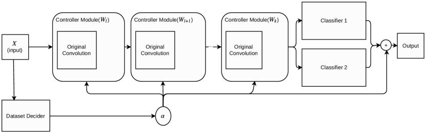
Figure 1: Overview of proposed method. For newly learned domains, controller modules are attached to convolutions of a base network, whose parameter are frozen. A switching variable $\alpha$ allows to switch the behavior of the network between the original behaviour of the convolution and a re-parametrized one for the new domain. $\alpha$ can be determined either manually or via a sub-network (“Dataset Decider”) which determines the source domain of the image, switching accordingly between different sets of control parameters. $\alpha$ Also controls which of the classifiers to apply. Other layers (e.g, non-linearities, batch-normalization, skip layers) not shown for presentation purposes. We visualize one added task, though an arbitrary number of tasks can be added.

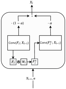
Figure 2: Controller modules: filters of a convolutional layer of a base network are modified by re-combining their weights through a controller module, where a switching $\alpha$ variable can choose between the original filters $F_{l}$ and newly created ones $F_{l}^{a}$. We show a controller module for a single added task, but any number of controllers can be added, with $\alpha$ then being a vector instead of scalar.

While deep neural networks continue to show remarkable performance gains in various areas such as image classification [1], semantic segmentation [2], object detection [3], speech recognition [4] medical image analysis [5] - and many more - it is still the case that typically, a separate model needs to be trained for each new task. Given two tasks of a totally different modality or nature, such as predicting the next word in a sequence of words versus predicting the class of an object in an image, it stands to reason that each would require a different architecture or computation. A more restricted scenario - and the one we aim to tackle in this work - is that of learning a representation which works well on several related domains. Such a scenario was recently coined by Rebuffi et al.[6] as multiple-domain learning (MDL) to set it aside from multi-task learning - where different tasks are to be performed on the same domain. An example of MDL is image-classification where the images may belong to different domains, such as drawings, natural images, etc. In such a setting it is natural to expect that solutions will:

1. Utilize the same computational pipeline

2. Require a modest increment in the number of required parameters for each added domain

3. Retain performance of already learned datasets (avoid “catastrophic forgetting”)

4. Be learned incrementally, dropping the requirement for joint training such as in cases where the training data for previously learned tasks is no longer available.

Our goal is to enable a network to learn a set of related tasks one by one while adhering to the above requirements. We do so by augmenting a network learned for one task with controller modules which utilize already learned representations for another. The parameters of the controller modules are optimized to minimize a loss on a new task. The training data for the original task is not required at this stage. The network’s output on the original task data stays exactly as it was; any number of controller modules may be added to each layer so that a single network can simultaneously encode multiple distinct domains, where the transition from one domain to another can be done by setting a binary switching variable or controlled automatically. The resultant architecture is coined DAN, standing for Deep Adaptation Networks. We demonstrate the effectiveness of our method on the recently introduced Visual Decathlon Challenge [6] whose task is to produce a classifier to work well on ten different image classification datasets. Though adding only 13% of the number of original parameters for each newly learned task (the specific number depends on the network architecture), the average performance surpasses that of fine tuning all parameters - without the negative side effects of doubling the number of parameters and catastrophic forgetting. In this work, we focus on image classification in various datasets, hence in our experiments the word “task” refers to a specific dataset/domain. The proposed method is extensible to multi-task learning, such as a single network that performs both image segmentation and classification, but this paper does not pursue this.

Our main contribution is the introduction of an improved alternative to transfer learning, which is as effective as fine-tuning all network parameters towards a new task, precisely preserves old task performance, requires a fraction (network dependent, typically 13%) of the cost in terms of new weights and is able to switch between any number of learned tasks. Experimental results verify the applicability of the method to a wide range of image-classification datasets.

We introduce two variants of the method, a fully-parametrized version, whose merits are described above and one with far fewer parameters, which significantly outperforms shallow transfer learning (i.e. feature extraction) for a comparable number of parameters. In the next section, we review some related work. Sec. 3 details the proposed method. In Sec. 4 we present various experiments, including comparison to related methods, as well as exploring various strategies on how to make our method more effective, followed by some discussion & concluding remarks.

2 Related Work

2.1 Multi-task Learning

In multi-task learning, the goal is to train one network to perform several tasks simultaneously on the same input. This is usually done by jointly training on all tasks. Such training is advantageous in that a single representation is used for all tasks. In addition, multiple losses are said to act as an additional regularizer. Some examples include facial landmark localization [7], semantic segmentation [8], 3D-reasoning [9], object and part detection [10] and others. While all of these learn to perform different tasks on the same dataset, the recent work of [11] explores the ability of a single network to perform tasks on various image classification datasets. We also aim to classify images from multiple datasets but we propose doing so in a manner which learns them one-by-one rather than jointly. Concurrent with our method is that of [6] which introduces dataset-specific additional residual units. We compare to this work in Sec 4. Our work bears some resemblance to [12], where two networks are trained jointly, with additional “cross-stitch” units, allowing each layer from one network to have as additional input linear combinations of outputs from a lower layer in another. However, our method does not require joint training and requires significantly fewer parameters.

2.2 Incremental Learning

Adding a new ability to a neural net often results in so-called “catastrophic forgetting” [13], hindering the network’s ability to perform well on old tasks. The simplest way to overcome this is by fixing all parameters of the network and using its penultimate layer as a feature extractor, upon which a classifier may be trained [14, 15]. While guaranteed to leave the old performance unaltered, it is observed to yield results which are substantially inferior to fine-tuning the entire architecture [3]. The work of Li and Hoiem [16] provides a succinct taxonomy of several variants of such methods. In addition, they propose a mechanism of fine-tuning the entire network while making sure to preserve old-task performance by incorporating a loss function which encourages the output of the old features to remain constant on newly introduced data. While their method adds a very small number of parameters for each new task, it does not guarantee that the model retains its full ability on the old task. Rusu et al.[17] shows new representations can be added alongside old ones while leaving the old task performance unaffected. However, this comes at a cost of duplicating the number of parameters of the original network for each added task. In Kirkpatrick et al.[18] the learning rate of neurons is lowered if they are found to be important to the old task. Our method fully preserves the old representation while causing a modest increase in the number of parameters for each added task. Recently, Sarwar et al.[19] have proposed to train a network incrementally by sharing a subset of early layers and splitting later ones. By construction, their method also preserves the old representation. However, as their experiments show, re-learning the parameters of the new network branches, whether initialized randomly with a similar distribution or simply copying the old ones results in worse performance than learning without any network sharing. Our method, while also re-utilizing existing weights, attains results which are on average better than simple transfer learning or learning from scratch.

2.3 Network Compression

Multiple works have been published on reducing the number weights of a neural network as a means to represent it compactly [20, 21], gain speedups [22] or avoid over-fitting [23], using combinations of coding, quantization, pruning and tensor decomposition. Such methods can be used in conjunction with ours to further improve results, as we show in Sec. 4.

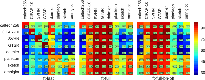
(a)

Figure 3: Transferability of various datasets to each other (ft-last) fine tuning only the last layer (full) fine-tuning all layers (ft-full-bn-off) fine tuning all layers while disallowing batch-normalization layers’ weights to be updated. Overall, networks tend to be more easily transferable to problems from related domains (e.g., natural / drawing). Zoom in to see numbers. It is recommended to view this figure in color on-line.

3 Approach

We begin with some notation. Let $T$ be some task to be learned. Specifically, we use a deep convolutional neural net (DCNN) in order to learn a classifier to solve $T$, which is an image classification task. Most contemporary DCNN’s follow a common structure: for each input $x$, the DCNN computes a representation of the input by passing it through a set of $l$ layers $\phi_{i}$, $i\in 1\ldots l$ interleaved with non-linearities. The initial (lower) layers of the network are computational blocks, e.g. convolutions with optional residual units in more recent architectures [24]. Our method applies equally to networks with or without residual connections. At least one fully connected layer $f_{i}$, $i\in 1\ldots c$ is attached to the output of the last convolutional layer. Let $\Phi_{F_{N}}=\sigma(\phi_{l})\circ\ldots\sigma(\phi_{2})\circ\sigma(\phi_{1})$ be the composition of all of the convolutional layers of the network $N$, interleaved by non-linearities. We use an architecture where all non-linearities $\sigma$ are the same function, with no tunable parameters. Denote by $\Phi_{F_{N}}(x)$ the feature part of $N$. Similarly, denote by $\Phi_{C_{N}}=f_{c}\circ\ldots\sigma(f_{2})\circ\sigma(f_{1})$ the classifier part of $N$, i.e. the composition of all of the fully-connected layers of $N$. The output of $N$ is then simply defined as:

$$N(x)=\Phi_{C_{N}}\circ\Phi_{F_{N}}(x)$$ (1)

We do not specify batch-normalization layers in the above notation for brevity. It is possible to drop the $\Phi_{C_{N}}$ term, if the network is fully convolutional, as in [2].

3.1 Adapting Representations

Assume that we are given two tasks, $T_{1}$ and $T_{2}$, to be learned, and that we have learned a base network $N$ to solve $T_{1}$. We assume that a good solution to $T_{2}$ can be obtained by a network with the same architecture as $N$ but with different parameters. We augment $N$ so that it will be able to solve $T_{2}$ as well by attaching a controller module to each of its convolutional layers. Each controller module uses the existing weights of the corresponding layer of $N$ to create new convolutional filters adapted to the new task $T_{2}$: for each convolutional layer $\phi_{l}$ in $N$, let $F_{l}\in\mathcal{R}^{C_{o}\times C_{i}\times k\times k}$ be the set of filters for that layer, where $C_{o}$ is the number of output features, $C_{l}$ the number of inputs, and $k\times k$ the kernel size (assuming a square kernel). Denote by $b_{l}\in\mathcal{R}^{C}$ the bias. Denote by $\tilde{F_{l}}\in\mathcal{R}^{C_{o}\times D}$ the matrix whose rows are flattened versions of the filters of $F_{l}$, where $D=C_{i}\cdot k\cdot k$; let $f\in\mathcal{R}^{C_{i}\times k\times k}$ be a filter from $F_{l}$ whose values are

$$f^{1}=\left(\begin{array}[]{ccc}f_{11}^{1}&\cdots&f_{1k}^{1}\\ &\ddots\\ &&f_{kk}^{1}\end{array}\right),\cdots,f^{i}=\left(\begin{array}[]{ccc}f_{11}^{i}&\cdots&f_{1k}^{i}\\ &\ddots\\ &&f_{kk}^{i}\end{array}\right)$$ (2)

The flattened version of $f$ is a row vector:

$$\tilde{f}=(f_{11}^{1},\cdots,f_{kk}^{1},\cdots,\cdots f_{11}^{i},\cdots,f_{kk}^{i})\in\mbox{$\mathcal{R^{D}}$}$$ (3)

“Unflattening” a row vector $\tilde{f}$ reverts it to its tensor form $f\in\mathcal{R}^{C_{i}\times k\times k}.$ This way, we can write

$$\tilde{F_{l}^{a}}=W_{l}\cdot\tilde{F_{l}}$$ (4)

where $W_{l}\in\mathcal{R}^{C_{o}\times C_{o}}$ is a weight matrix defining linear combinations of the flattened filters of $F_{l}$, resulting in $C_{o}$ new filters. Unflattening $\tilde{F_{l}^{a}}$ to its original shape results in $F_{l}^{a}\in\mathcal{R}^{C_{o}\times C_{i}\times k\times k}$, which we call the adapted filters of layer $\phi_{l}$. Using the symbol $X\otimes Y$ as shorthand for flatten $Y$$\rightarrow$matrix multiply by $X$$\rightarrow$unflatten, we can write:

$$F_{l}^{a}=W_{l}\otimes F_{l}$$ (5)

If the convolution contains a bias, we instantiate a new weight vector $b_{l}^{a}$ instead of the original $b_{l}$. The output of layer $\phi_{l}$ is computed as follows: let $x_{l}$ be the input of $\phi_{l}$ in the adapted network. For a given switching parameter $\alpha\in\{0,1\}$, we set the output of the modified layer to be the application of the switched convolution parameters and biases:

$$x_{l+1}=[\alpha(W_{l}\otimes F_{l})+(1-\alpha)F_{l}]\ast x_{l}+\alpha b_{l}^{a}+(1-\alpha)b_{l}$$ (6)

The above formulation is for switching between two different behaviours - that of a base network and that of the controller modules learned for a new task.

To allow the network to perform multiple tasks, we turn $\alpha$ to a vector $\alpha\in\{0,1\}^{n}$ where $n$ is the overall number of tasks, so that $\alpha_{j}=1$if we want to perform the $j$’th task and 0 otherwise. The output of the $l$ layer will be then determined similarly to Equation 6:

$$x_{l+1}={\sum}_{i=1}^{n}\alpha_{i}(F_{l}^{a_{i}}\ast x_{l}+b_{l}^{i})$$

Where $F_{l}^{a_{i}}$, $b_{l}^{i}$ are the set of adapted filters / bias for the $i$’th task and we define for $F_{l}^{a_{1}}=F_{l},b_{l}^{1}=b_{l}$ to include the original task.

A set of fully connected layers $f_{i}^{a}$ are learned from scratch, attaching a new “head” to the network for each new task. Throughout training & testing, the weights of $F$ (the filters of $N$) are kept fixed and serve as basis functions for $F^{a}$. The weights of the controller modules are learned via back-propagation given the loss function. Weights of any batch normalization (BN) layers are either kept fixed or learned anew. The batch-normalized output is switched between the values of the old and new BN layers, similarly to Eq. 6. A visualization of the resulting DAN can be seen in Fig. 1 and a single control module in Fig. 2.

Net	C-10	GTSR	SVHN	Caltech	Dped	Oglt	Plnk	Sketch	Perf.	#par
VGG-B(S)	92.5	98.2	96.2	88.2	92.9	86.9	74.5	69.2	87.32	8
VGG-B(P)	93.2	99.0	95.8	92.6	98.7	83.8	73.2	65.4	87.71	8
$\mathbf{DAN}_{\mathbf{caltech-256}}$	77.9	93.6	91.8	88.2	93.8	81.0	63.6	49.4	79.91	2.54
$DAN_{sketch}$	77.9	93.3	93.2	86.9	94.0	85.4	69.6	69.2	83.7	2.54
$DAN_{noise}$	68.1	90.9	90.4	84.6	91.3	80.6	61.7	42.7	76.29	1.76
$DAN_{imagenet}$	91.6	97.6	94.6	92.2	98.7	81.3	72.5	63.2	86.46	2.76
$DAN_{imagenet+sketch}$	91.6	97.6	94.6	92.2	98.7	85.4	72.5	69.2	87.76	3.32

TABLE I: Perf: top-1 accuracy (%, higher is better) on various datasets and parameter cost (#par., lower is better) for a few baselines and several variants of our method. Rows 1,2: independent baseline performance. VGG-B: VGG [25] architecture B. (S) - trained from scratch. (P) - pre-trained on ImageNet. Rows 3-7: (ours) controller network performance; $DAN_{sketch}$ as a base network outperforms $DAN_{caltech-256}$ on most datasets. A controller network based on random weights ($DAN_{noise}$) works quite well given that its number of learned parameters is a fifth of the other methods. $DAN_{imagenet}$: controller networks initialized from VGG-B model pretrained on ImageNet. $DAN_{imagenet+sketch}$: selective control network based on both VGG-B(P) & Sketch. We color code the first, second and third highest values in each column (lowest for #par). #par: amortized number of weights learned to achieve said performance for all tasks divided by number of tasks addressed (lower is better).

We denote a network learned for a dataset/task $S$ as $N_{S}$. A controller learned using $N_{S}$ as a base network will be denoted as $DAN_{S}$, where DAN stands for Deep Adaptation Network and $DAN_{S\rightarrow T}$ means using $DAN_{S}$ for a specific task $T$. While in this work we apply the method to classification tasks it is applicable to other tasks as well.

3.2 Additional Design Choices

In the following, we mention some additional design choices of possible ways to augment a network with controllers, as well as provide some analysis on the incurred cost of parameters.

3.2.1 Weaker parametrization

A weaker variant of our method is one that forces the matrices $W_{l}$ to be diagonal, e.g, only scaling the output of each filter of the original network. We call this variant “diagonal” (referring only to scaling coefficients, such as by a diagonal matrix) and the full variant of our method “linear” (referring to a linear combination of filters). The diagonal variant can be seen as a form of explicit regularization which limits the expressive power of the learned representation. While requiring significantly fewer parameters, it results in poorer classification accuracy, but as will be shown later, also outperforms regular feature-extraction for transfer learning, especially in network compression regimes.

3.2.2 Multiple Controllers

The above description mentions one base network and one controller network. However, any number of controller networks can be attached to a single base network, regardless of already attached ones. In this case $\alpha$ is extended to one-hot vector of values determined by another sub-network, allowing each controller network to be switched on or off as needed.

3.2.3 Parameter Cost

The number of new parameters added for each task depends on the number of filters in each layer and the number of parameters in the fully-connected layers. As the latter are not reused, their parameters are fully duplicated. Let $M=C_{o}\times D$ be the filter dimensions for some conv. layer $\phi_{l}$ where $D=C_{i}\times k\times k$. A controller module for $\phi_{l}$ requires $C_{o}^{2}$ coefficients for $F_{l}^{a}$ and an additional $C_{o}$ for $b_{l}^{a}$. Hence the ratio of new parameters w.r.t to the old for $\phi_{l}$ is $\frac{C_{o}\times(C_{o}+1)}{C_{o}\times(D+1)}=\frac{C_{o}+1}{D+1}\approx\frac{C_{o}}{D}$. Example: for $C_{o}=C_{i}=256$ input and output units and a kernel size $k=5$ this equals $\frac{256+1}{256\cdot 5^{2}+1}\approx 0.04$. In the final architecture we use the total number of weights required to adapt the convolutional layers $\Phi_{l}$ combined with a new fully-connected layer amounts to about 13% of the original parameters. For VGG-B, this is roughly 21%. For instance, constructing 10 classifiers using one base network and 9 controller networks requires $(1+0.13*9)\cdot P$=$2.17\cdot P$ parameters where $P$ is the number for the base network alone, compared to $10\cdot P$ required to train each network independently. The cost is dependent on network architecture, for example it is higher when applied on the VGG-B architecture. While our method can be applied to any network with convolutional layers, if $C_{o}\geq D$, i.e., the number of output filters is greater than the dimension of each input filter, it would only increase the number of parameters.

3.3 Limitations

An immediate question that arises from our formulation concerns the expressive power of the resulting adapted networks. We provide some analysis here on this issue. In regular fine-tuning or learning schemes, the weights of each layer may take on arbitrary values, depending on the optimization scheme and training data. In contrast, the proposed method constrains each filter to be a linear combination of the original filters in the corresponding layer. This may, in general, become a strong limiting factor on the performance of the network. The filters $F=f_{1},\dots,f_{k}$ of a layer $l$ can form vectors by flattening their tensor form. $F$ defines a basis of a subspace of filters from which the proposed method creates new ones. As our method defines new filters by applying a linear transformation on $F$, the initial values thereof can have several effects on the resulting networks. Two important scenarios are when (a) network expressibility and (b) network efficiency are affected. We provide examples of when these scenarios can occur and some experiments to demonstrate them.

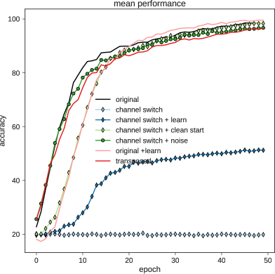
(a)

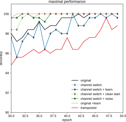
(b)

Figure 4: Demonstration of different possible limits of possible method on a toy example. Transferring from a network where the first layer contains features from an orthogonal sub-space to that required for a task can result in chance accuracy. Please see text for details.

3.3.1 Expressibility

One can easily construct cases where the expressive power of a network is critically hindered by choosing to adapt it from an inappropriate base network. For example, assume that the inputs of a network are RGB images. Also assume that - for some reason - all first-layer filters have coefficients of exactly 0 in the green and blue channels. If information in these channels is critical for the task to be learned by the proposed method, it will clearly fail, as the information resides in an orthogonal feature space to that represented by the base network’s filters.

Residual Connections

The above claim does not hold for networks with residual connections [24]. In Residual connections the output $y_{i}$ of the $i^{\prime}th$ layer is of the following general form:

$$y_{i}=F(x_{i};W_{i})+x_{i}$$ (7)

where $x_{i}$ is the input to this layer and $W_{i}$ is the layer’s parameters. This allows preserving information from the previous layer, as a possible function permitted by this is the identity function. If enough information from the signal $x$ is preserved then the next layer can still recover from not representing it adequately in this layer. Hence, the expressive power of the network is probably less sensitive to the choice of basis function in a single layer. Nevertheless, its efficiency may be compromised, as we describe next.

3.3.2 Efficiency

In some cases, the expressive power of the network is not immediately affected by the choice of basis function but we claim that the efficiency of the network is. We define the efficiency of a network w.r.t to a given image patch as the minimal number of layers (depth) required to discriminate it from others by a single filter. In other words, the depth of the shallowest layer where there exists some filter whose response correlates strongly with the presence of the patch. An example is a 3x3 gray-scale patch with 1 in all corners and 0 otherwise. In the first layer, a filter $v$ of values:

$$v=\left(\begin{array}[]{ccc}+1&-1&+1\\ -1&-1&-1\\ +1&-1&+1\end{array}\right)$$

would perfectly match this patch. On the other hand, one could set 9 filters of the first layer to delta functions with 1 in location $i,j$ for each $i$ and $j$ in ${{1,2,3}}.$ These filters span all possible patches of 3x3 so they do not effect expressibility. However, keeping the first layer fixed, the second layer would be required to create a filter to match $p$, whereas $v$ expressed this directly.

3.3.3 Toy Dataset

To further demonstrate the above claims, we constructed a toy classification task. We first describe the dataset and experiments and then discuss the results.

The task is: given an input image of size 28x28x3, predict the length of a bar in the an image. In this dataset, the images are restricted to be 1-pixel width bars of length $3\cdot k$ where $k\in\{3,4,5,6,7\}$ over a blank background and the class is the corresponding length of the bar. The bar lengths were set to be in increments of 3 as lesser ones caused difficulties for the network to learn, probably due to max-pooling operations.

The dataset is composed of 1000 examples, with a random 75%/25% train/test split. The network we tested is deliberately quite degenerate: it contains one 5x5 filter on the first layer and 20 filters on the second, followed by two fully connected layers of 320x50 and 50x5.

We created 3 variants of this dataset, to test different transfer-learning scenarios on it. The dataset variants are (1) only red horizontal bars, (2) only red vertical bars (referred to as “transposed”) and (3) only green horizontal bars (referred to as “new channel”). Note that we limited our method to operate only on the first layer, which in this case boils down to multiplying the output of the filter by a scalar and learning a new bias.

The network was trained for 50 epochs using the Adam [26] optimizer (SGD did not converge as well in this case) in all scenarios. We tested seven scenarios. These involve different combinations of the images in the dataset, initialization of the first layer and which layers may or may not be modified by the optimizer.

• original: horizontal dataset, first filter fixed to a horizontal green bar, learn other layers

• original+learn : horizontal dataset, learn all layers

• transposed : transposed dataset, first filter fixed to a horizontal bar, learn other layers

• channel switch: new channel dataset, first filter fixed to horizontal green bar, learn other layers

• channel switch + noise: new channel dataset, first filter fixed to horizontal green bar+ Gaussian noise, learn other layers

• channel switch + clean start: new channel dataset, learn all layers

• channel switch + learn: new channel dataset, first filter initialized to a horizontal green bar, learn all layers.

Each experiment was repeated 20 times to account for variability. We plot the mean accuracy on the validation set over the 50 training epochs.

Fig. 4 summarizes the result of these experiments. The left sub-figure shows the mean performance over the 50 epochs and the right one shows the maximal (of the 20 trials) attained for each scenario. These show that in most cases, we can reach good accuracy, however on the average case there are drastic differences between the obtained performance, although this is a very simple dataset. The original scenario, where the first layer is fixed, attains 100% accuracy. Switching the channel from green to red (“channel switch”) but keeping the first filter fixed results in chance accuracy, as excepted: no linear combination of a purely “green” filter can represent information from the red channel. In this case, if we allow all layers to be learned (“channel switch + learn”), indeed the network can finally converge to a good accuracy (Fig. 4 (b)), but the average performance over 20 trials is far from optimal (Fig. 4 (a)) - the network converges to around 50% accuracy (where chance performance is 20%). This confirms that even for very simple cases, bad initialization can be detrimental to the training process.

As a “sanity test”, we make sure that randomly initializing the network and allowing all layers to be learned in the “channel switch” case achieves 100% performance (in both the average and best case). This is indeed the case (“channel switch + clean start”), although we see that the random initialization converges at first much slower than the informed initialization of “original”. Next, we initialize the network as in “original” but with the “channel switch” dataset. However, we add random noise to the first layer’s filter, then keep it fixed (“channel switch + noise”). The optimization is able to recover from this initialization in both the average and best case, as the initial filter is not orthogonal to the green channel.

The “original + learn” is initialized as “original” but allows the first layer to be modified. While on average it initially converges slower than the “original” scenario, on average it performs better.

Finally, the “transposed” case, where the original filter is fixed to be orthogonal to the required shape (horizontal bars), attains average lower performance, and near 100% in the best case. Note that although we cannot generate an horizontal bar by linearly transforming the vertical one, the information is not lost and can be recovered by filters of the second layer, due to their convolutional nature. This is done by a weighted summation of the shifted responses of the horizontal filter with proper coefficients. This is an example of the network “efficiency” being reduced, i.e, delegating to the second layer computations which could be done in the first.

To summarize, we conclude from the experiments on this toy dataset that:

1. Setting some network weights using strong domain-specific knowledge and fixing their values, learning only other layers can lead to fast convergence to a strong solution.

2. An even stronger solution can emerge if all layers are initialized randomly, then allowed to be updated - though convergence will be slower.

3. Initializing some weights to “bad” values can cause on-average dramatically inferior performance to the previous two cases, with occasional but rare instances of good performance.

4. Initializing some weights to “bad” values, fixing them and learning the rest of the weights will totally and irreparably prevent the network from learning.

In the next section, we test our method on richer and more diverse datasets, less degenerate networks (e.g., more than one filter in the first layer), and in some cases residual networks, which all are likely to diminish effects shown on artificial examples.

4 Experiments on Real Datasets

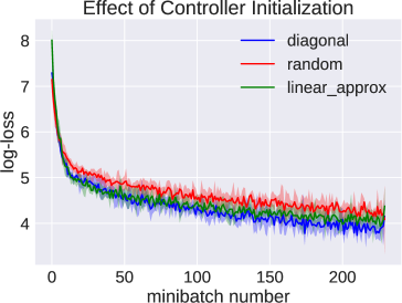
(a)

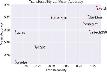
(b)

Figure 5: (a) Controller initialization schemes. Mean loss averaged over 5 experiments for different ways of initializing controller modules, overlaid with minimal and maximal values. Random initialization performs the worst (random). Approximating the behavior of a fine-tuned network is slightly better (linear_approx) and initializing by mimicking the base network (diagonal) performs the best (b) Predictability of a control network’s overall accuracy average over all datasets, given its transferability measure.

We conduct several experiments to test our method and explore different aspects of its behavior. The experimental section is split into two parts, the first being of a more exploratory nature and the second geared toward results in a recent multi-task learning benchmark. We use two different basic network architectures on two (somewhat overlapping) sets of classification benchmarks for the respective parts. The first is VGG-B [25] . We begin by listing the datasets we used (4.0.1), followed by establishing baselines by training a separate model for each using a few initial networks. We proceed to test several variants of our proposed method (4.1) as well as testing different training schemes. Next, we discuss methods of predicting how well a network would fare as a base-network (4.3). We show how to discern the domain of an input image and output a proper classification (4.3.1) without manual choice of the control parameters $\alpha$. In the second part of our experiments we show how our applying our method results in leading scores in the Visual Decathlon Challenge [6], using a different, more recent architecture. Before concluding we demonstrate some useful properties of our method.

All Experiments were performed using the PyTorch framework using a single Titan-X Pascal GPU.

Dataset	DPed	SVHN	GTSR	C-10	Oglt	Plnk	Sketch	Caltech
ft-full	60.1	60	65.8	70.9	80.4	81.6	84.2	82.3
ft-full-bn-off	61.8	64.6	66.2	72.5	78	80.2	82.5	81
ft-last	24.4	33.9	42.5	44	44.1	47	50.3	55.6

TABLE II: Mean transfer learning performance. We show the mean top-1 accuracy (%) attained by fine-tuning a network from each domain to all domains. Out of the datasets above, starting with Caltech-256 proves most generic as a feature extractor (ft-last). However, fine tuning is best when initially training on the Sketch dataset (ft-full).

4.0.1 Datasets and Evaluation

The first part of our evaluation protocol resembles that of [11]: we test our method on the following datasets: Caltech-256 [27], CIFAR-10 [28], Daimler [29] (DPed), GTSR [30], Omniglot [31], Plankton imagery data [32] (Plnk), Human Sketch dataset [33] and SVHN [34]. All images are resized to 64 × 64 pixels, duplicating gray-scale images so that they have 3 channels as do the RGB ones. We whiten all images by subtracting the mean pixel value and dividing by the variance per channel. This is done for each dataset separately. We select 80% for training and 20% for validation in datasets where no fixed split is provided. We use the B architecture described in [25], henceforth referred to as VGG-B. It performs quite well on the various datasets when trained from scratch (See Tab. I. Kindly refer to [11] for a brief description of each dataset.

As a baseline, we train networks independently on each of the 8 datasets. All experiments in this part are done with the Adam optimizer [26], with an initial learning rate of 1e-3 or 1e-4, dependent on a few epochs of trial on each dataset. The learning rate is halved after each 10 epochs. Most networks converge within the first 10-20 epochs, with mostly negligible improvements afterwards. We chose Adam for this part due to its fast initial convergence with respect to non-adaptive optimization methods (e.g, SGD), at the cost of possibly lower final accuracy [35]. The top-1 accuracy (%) is summarized in Table I.

4.1 Controller Networks

To test our method, we trained a network on each of the 8 datasets in turn to be used as a base network for all others. We compare this to the baseline of training on each dataset from scratch (VGG-B(S)) or pretrained (VGG-B(P)) networks. Tab. I summarizes performance on all datasets for two representative base nets: $DAN_{caltech-256}$ (79.9%) and $DAN_{sketch}$ (83.7%). Mean performance for other base nets are shown in Fig. 5 (a). The parameter cost (3.2.3) of each setting is reported in the last column of the table. This (similarly to [6] is the total number of parameters required for a set of tasks normalized by that of a single fully-parametrized network. We also check how well a network can perform as a base-network after it has seen ample training examples: $DAN_{imagenet}$ is based on VGG-B pretrained on ImageNet [36]. This improves the average performance by a significant amount (83.7% to 86.5%). On Caltech-256 we see an improvement from 88.2% (training from scratch). However, for both Sketch and Omniglot the performance is in favor of $DAN_{sketch}$. Note these are the only two domains of strictly unnatural images. Additionally, $DAN_{imagenet}$ is still slightly inferior to the non-pretrained VGG-B(S) (86.5% vs 87.7%), though the latter is more parameter costly.

4.1.1 Multiple Base Networks

Arguably, a good base network should have features generic enough so that a controller network can use them for a broad range of target tasks. In practice this may not necessarily be the case. We conjecture that using a diverse set of features, such as that learned by training on more than one task, will provide a better basis for transfer learning. To use two base-networks simultaneously, we implemented a dual-controlled network by using both $DAN_{caltech-256}$ and $DAN_{sketch}$ and attaching to them controller networks. The outputs of the feature parts of the resulting sub-networks were concatenated before the fully-connected layer. This resulted in the exact same performance as $DAN_{sketch}$ alone. However, by using selected controller-modules per group of tasks, we can improve the results: for each dataset the maximally performing network (based on validation) is the basis for the control module, i.e., we used $DAN_{imagenet}$ for all datasets except Omniglot and Sketch. For the latter two we use $DAN_{sketch}$ as a base net. We call this network $DAN_{imagenet+sketch}$. At the cost of more parameters, it boosts the mean performance to 87.76% - better than using any single base net for controllers or training from scratch. Since it is utilized for 9 tasks (counting ImageNet), its parameter cost (2.76) is still quite good.

4.1.2 Starting from a Randomly Initialized Base Network

We tested how well our method can perform without any prior knowledge, e.g., building a controller network on a randomly initialized base network. The total number of parameters for this architecture is ~12M. However, as 10M have been randomly initialized and only the controller modules and fully-connected layers have been learned, the effective number is actually 2M. Hence its parameter cost is determined to be 0.22. We summarize the results in Tab. I. Notably, the results of this initialization worked surprisingly well; the mean top-1 precision attained by this network was 76.3%, slightly worse than of $DAN_{caltech-256}$ (79.9%). This is better than initializing with $DAN_{daimler}$, which resulted in a mean accuracy of 75%. This is possible because the random values in the base network can still be linearly combined by our method to create ones that are useful for classification.

4.2 Initialization

One question which arises is how to initialize the weights $W$ of a control-module. We tested several options: (1) Setting $W$ to an identity matrix (diagonal). This is equivalent to the controller module starting with a state which effectively mimics the behavior of the base network (2) Setting $W$ to random noise (random) (3) Training an independent network for the new task from scratch, then set $W$ to best linearly approximate the new weights with the base weights (linear_approx). To find the best initialization scheme, we trained $DAN_{sketch\rightarrow caltech256}$ for one epoch with each and observed the loss. Each experiment was repeated 5 times and the results averaged. From Fig. 5(a), it is evident that the diagonal initialization is superior, perhaps counter-intuitively, there is no need to train a fully parametrized target network. Simply starting with the behavior of the base network and tuning it via the control modules results in faster convergence. Hence we train controller modules with the diagonal method. Interestingly, the residual adaptation unit in [6] is initially similar to the diagonal configuration. If all of the filters in their adapter unit are set to 1 (up to normalization), the output of the adapter will be initially the same as that of the controller unit initialized with the identity matrix.

4.3 Transferability

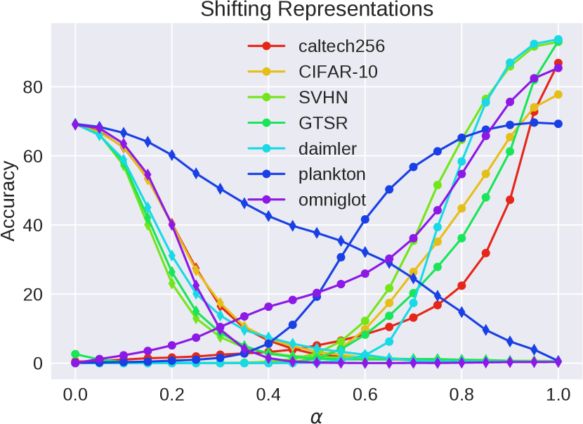
Figure 6: Shifting Representations. Using a single base network $N_{sketch}$, we check the method’s sensitivity to varying values of $\alpha$ by varying it in the range $[0,1]$. Increasing $\alpha$ shifts the network away from the base representation and towards learned tasks - gradually lowering performance on the base task (diamonds) and improving on the learned ones (full circles). The relatively slow decrease of the performance on sketch (blue diamonds) and increase in that of Plankton (blue circles) indicates a similarity between the learned representations.

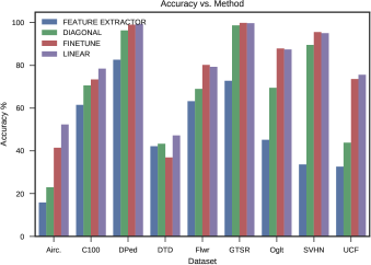
(a)

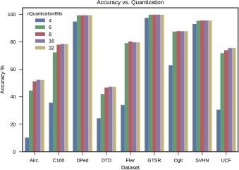
(b)

Figure 7: (a) Accuracy vs. learning method. Using only the last layer (feature extractor) performs worst. finetune: vanilla fine-tuning. Diagonal : our controller modules with a diagonal combination matrix. Linear: our full method. On average, our full method outperforms vanilla fine tuning. (b) Accuracy vs. quantization: with as low as 8 bits, we see no significant effect of network quantization on our method, showing they can be applied together.

How is one to choose a good network to serve as a base-network for others? As an indicator of the representative power of the features of each independently trained network $N$, we test the performance on other datasets, using $N$ for fine tuning. We define the transferability of a source task $S$ w.r.t a target task $T$ as the top-1 accuracy attained by fine-tuning $N$ trained on $S$ to perform on $T$. We test 3 different scenarios, as follows: (1) Fine-tuning only the last layer (a.k.a feature extraction) (ft-last); (2) Fine-tuning all layers of $N$(ft-full); (3) same as ft-full, but freezing the parameters of the batch-normalization layers - this has proven beneficial in some cases - we call this option ft-full-bn-off. The results in Fig 3 show some interesting phenomena. First, as expected, feature extraction (ft_last) is inferior to fine-tuning the entire network. Second, usually training from scratch is the most beneficial option. Third, we see a distinction between natural images (Caltech-256, CIFAR-10, SVHN, GTSR, Daimler) and unnatural ones (Sketch, Omniglot, Plankton); Plankton images are essentially natural but seem to exhibit different behavior than the rest.

It is evident that features from the natural images are less beneficial for the unnatural images. Interestingly, the converse is not true: training a network starting from Sketch or Omniglot works quite well for most datasets, both natural and unnatural. This is further shown in Tab. II: we calculate the mean transferability of each dataset by the mean value of each rows of the transferability matrix from Fig. 3. $DAN_{Caltech-256}$ works best for feature extraction. However, for full fine-tuning using $DAN_{Plankton}$ works as the best starting point, closely followed by $DAN_{Caltech-256}$. For controller networks, the best mean accuracy attained for a single base net trained from scratch is attained using $DAN_{sketch}$ (83.7%). This is close to the performance attained by full transfer learning from the same network (84.2%, see Tab. II) at a fraction of the number of parameters. This is consistent with our transferability measure. To further test the correlation between the transferability and the performance given a specific base network, we used each dataset as a base for control networks for all others and measured the mean overall accuracy. The results can be seen in Fig. 5 (b).

4.3.1 A Unified Network

Finally, we test the possibility of a single network which can both determine the domain of an image and classify it. We train a classifier to predict from which dataset an image originates, using the training images from the 8 datasets. This is learned easily by the network (also VGG-B) which rapidly converges to 99% accuracy. With this “dataset-decider”, named $N_{dc}$ we augment $DAN_{sketch}$ to set for each input image $I$ from any of the datasets $D_{i}$ the controller value $\alpha_{i}$ of $DAN_{sketch\rightarrow D_{i}}$ to 1 if and only if $N_{dc}$ deemed $I$ to originate from $D_{i}$ and to 0 otherwise. This produces a network which applies to each input image the correct controllers, classifying it within its own domain. While the predicted values of $\alpha_{i}$ are real-valued, we set the highest one to 1 and the rest to zero.

4.4 Visual Decathlon Challenge

We now show results on the recent Visual Decathlon Challenge of [6]. The challenge introduces involves 10 different image classification datasets: ImageNet [36]; Aircraft [37]; Cifar-100 [28]; Daimler Pedestrians [29]; Dynamic Textures [38]; GTSR [30]; Flowers [39]; Omniglot [40]; SVHN [34] and UCF-101 [41]. The goal is to achieve accurate classification on each dataset while retaining a small model size, using the train/val/test splits fixed by the authors. All images are resized so the smaller side of each image is 72 pixels. The classifier is expected to operate on images of 64x64 pixels. Each entry in the challenge is assigned a decathlon score, which is a function designed to highlight methods which do better than the baseline on all 10 datasets. Please refer to the challenge website for details about the scoring and datasets: http://www.robots.ox.ac.uk/~vgg/decathlon/. Similarly to [6], we chose to use a wide residual network [42] with an overall depth of 28 and a widening factor of 4, with a stride of 2 in the convolution at the beginning of each basic block. In what follows we describe the challenge results, followed by some additional experiments showing the added value of our method in various settings. In this section we used the recent YellowFin optimizer [43] as it required less tuning than SGD. We use an initial learning rate factor of 0.1 and reduce it to 0.01 after 25 epochs. This is for all datasets with the exception of ImageNet which we train for 150 epochs with SGD with an initial learning rate of 0.1 which is reduced every 35 epochs by a factor of 10. This is the configuration we determined using the available validation data which was then used to train on the validation set as well (as did the authors of the challenge) and obtain results from the evaluation server. Here we trained on the reduced resolution ImageNet from scratch and used the resulting net as a base for all other tasks. Tab. III summarizes our results as well as baseline methods and the those of [6], all using a base architecture of similar capacity. By using a significantly stronger base architecture they obtained higher results (mean of 79.43%) but with a parameter cost of 12, i.e., requiring 12 times the amount of original parameters. All of the rows are copied from [6], including their re-implementation of LWF, except the last which shows our results. The final column of the table shows the decathlon score. A score of 2500 reflects the baseline resulting from finetuning the network learned on ImageNet to each dataset independently. For the same architecture, the best results obtained by the Residual Adapters method is slightly below ours in terms of decathlon score and slightly above them in terms of mean performance. However, unlike them, we avoid joint training over all of the datasets and using dataset-dependent weight decay.

Method	#par	ImNet	Airc.	C100	DPed	DTD	GTSR	Flwr	Oglt	SVHN	UCF	mean	S
Scratch	10	59.87	57.1	75.73	91.2	37.77	96.55	56.3	88.74	96.63	43.27	70.32	1625
Feature	1	59.67	23.31	63.11	80.33	45.37	68.16	73.69	58.79	43.54	26.8	54.28	544
Finetune	10	59.87	60.34	82.12	92.82	55.53	97.53	81.41	87.69	96.55	51.2	76.51	2500
LWF	10	59.87	61.15	82.23	92.34	58.83	97.57	83.05	88.08	96.1	50.04	76.93	2515
Res. Adapt.	2	59.67	56.68	81.2	93.88	50.85	97.05	66.24	89.62	96.13	47.45	73.88	2118
Res. Adapt (Joint)	2	59.23	63.73	81.31	93.3	57.02	97.47	83.43	89.82	96.17	50.28	77.17	2643
DAN (Ours)	2.17	57.74	64.12	80.07	91.3	56.54	98.46	86.05	89.67	96.77	49.38	77.01	2851

TABLE III: Results on Visual Decathlon Challenge. Scratch: training on each task independently. Feature: using a pre-trained network as a feature extractor. Finetune : vanilla fine tuning. Performs well but requires many parameters. Learning-without-forgetting (LWF, [16] slightly outperforms it but with a large parameter cost. Residual adapt. [6] significantly reduce the number of parameters. Results improve when training jointly on all task (Res.Adapt(Joint)). The proposed method (DAN) outperforms residual adapters despite adding each task independently of the others. S is the decathlon challenge score.

4.5 Compression and Convergence

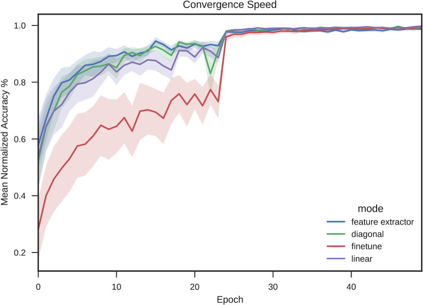
(a)

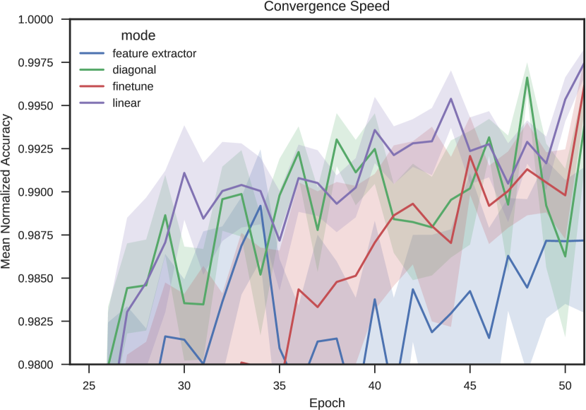
(b)

Figure 8: (a) Our method (linear) converges to a high accuracy faster than fine-tuning. The weaker variant of our method converges as fast as feature-extraction but reaches an overall higher accuracy (7 (a)). (b) zoom in on top-right of (a).

In this section, we highlight some additional useful properties of our method. All experiments in the following were done using the same architecture as in the last section but training was performed only on the training sets of the Visual Decathlon Challenge and tested on the validation sets. First, we check whether the effects of network compression are complementary to ours or can hinder them. Despite the recent trend of sophisticated network compression techniques (for example [20]) we use only a simple method of compression as a proof-of-concept, noting that using recent compression methods will likely produce better results. We apply a simple linear quantization on the network weights, using either 4, 6, 8, 16 or 32 bits to represent each weight, where 32 means no quantization. We do not quantize batch-normalization coefficients. Fig. 7 (b) shows how accuracy is affected by quantizing the coefficients of each network. Using 8 bits results in only a marginal loss of accuracy. This effectively means our method can be used to learn new tasks while requiring an addition of 3.25% of the original amount of parameters. Many maintain performance even at 6 bits (DPed, Flowers, GTSR, Omniglot, SVHN. Next, we compare the effect of quantization on different transfer methods: feature extraction, fine-tuning and our method (both diagonal and linear variants). For each dataset we record the normalized (divided by the max.) accuracy for each method/quantization level (which is transformed into the percentage of required parameters). This is plotted in Fig. 9. Our method requires significantly fewer parameters to reach the same accuracy as fine-tuning. If parameter usage is limited, the diagonal variant of our method significantly outperforms feature extraction. Finally, we show that the number of epochs until nearing the maximal performance is markedly lower for our method. This can be seen in Fig. 8.

4.6 Discussion

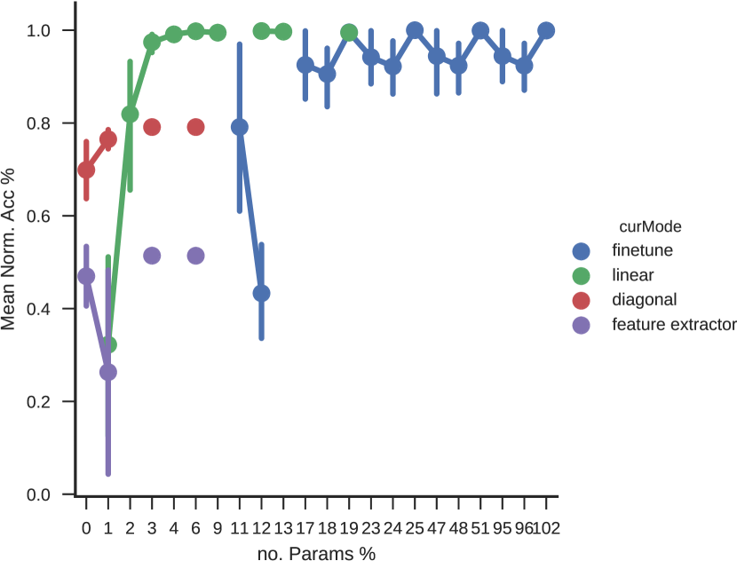
Figure 9: Mean classification accuracy (normalized, averaged over datasets) w.r.t no. parameters. Our method achieve better performance over baselines for a large range of parameter budgets. For very few parameters diagonal (ours) outperforms features extraction. To obtain maximal accuracy our full method requires far fewer parameters (see linear vs finetune).

We have observed that the proposed method converges to a reasonably good solution faster than vanilla fine-tuning and eventually attains slightly better performance. The increase in classification accuracy is despite the network’s expressive power, which is limited by our construction. We conjecture that constraining each layer to be expressed as a linear combination of the corresponding layer in the original network serves to regularize the space of solutions and is beneficial when the tasks are sufficiently related to each other. One could come up with simple examples where the proposed method would likely fail. This might occur if tasks are not of the same kind. For example, one task requires counting of horizontal lines and the other requires counting of vertical ones, and such examples are all that appear in the training sets, then the proposed method will likely work far worse than vanilla fine-tuning or training from scratch. We experimented with such scenarios in Sec. 3.3. Empirically, we did not see this happen in any of our experiments on “real” datasets. This may simply stem from some inherent similarity in image classification tasks which makes some basic set of features useful for most of them. We leave the investigation of this issue, as well as finding ways between striking a balance between reusing features and learning new ones as future work.

5 Conclusions

We have presented a method for transfer learning thats adapts an existing network to new tasks while fully preserving the existing representation. Our method matches or outperforms vanilla fine-tuning, though requiring a fraction of the parameters, which when combined with net compression reaches 3% of the original parameters with no loss of accuracy. The method converges quickly to high accuracy while being on par or outperforming other methods with the same goal. Built into our method is the ability to easily switch the representation between the various learned tasks, enabling a single network to perform seamlessly on various domains. The control parameter $\alpha$ can be cast as a real-valued vector, allowing a smooth transition between representations of different tasks. An example of the effect of such a smooth transition can be seen in Fig. 6 where $\alpha$ is used to linearly interpolate between the representation of differently learned pairs tasks, allowing one to smoothly control transitions between different behaviors. Allowing each added task to use a convex combination of already existing controllers will potentially utilize controllers more efficiently and decouple the number of controllers from the number of tasks.

Amir Rosenfeld received his B.Sc in Computer-Engineering at the Hebrew University of Jerusalem (HUJI) at 2006 and his M.Sc. in Computer Science at HUJI in 2011. He completed his PhD in Computer Science at the Weizmann Institute under the supervision of Prof. Shimon Ullman in 2016. He is currently a postdoctoral fellow at the Laboratory for Active and Attentive Vision, York University. His main research interests include machine learning, computer and human vision, visual attention and adaptive learning systems.

John K. Tsotsos is Distinguished Research Professor of Vision Science at York University. He received his doctorate in Computer Science from the University of Toronto. After a postdoctoral fellowship in Cardiology at Toronto General Hospital, he joined the University of Toronto on faculty in Computer Science and in Medicine. In 1980 he founded the Computer Vision Group at the University of Toronto, which he led for 20 years. He was recruited to York University in 2000 as Director of the Centre for Vision Research. He has been a Canadian Heart Foundation Research Scholar, Fellow of the Canadian Institute for Advanced Research and Canada Research Chair in Computational Vision. He received many awards and honours including several best paper awards, the 2006 Canadian Image Processing and Pattern Recognition Society Award for Research Excellence and Service, the 1st President’s Research Excellence Award by York University in 2009, and the 2011 Geoffrey J. Burton Memorial Lectureship from the United Kingdom’s Applied Vision Association for significant contribution to vision science. He was elected as Fellow of the Royal Society of Canada in 2010 and was awarded its 2015 Sir John William Dawson Medal for sustained excellence in multidisciplinary research, the first computer scientist to be so honoured. Over 125 trainees have passed through his lab. His current research focuses on a comprehensive theory of visual attention in humans. A practical outlet for this theory embodies elements of the theory into the vision systems of mobile robots.

References

- [1] A. Krizhevsky, I. Sutskever, and G. E. Hinton, “Imagenet classification with deep convolutional neural networks,” in Advances in neural information processing systems, 2012, pp. 1097–1105.
- [2] J. Long, E. Shelhamer, and T. Darrell, “Fully convolutional networks for semantic segmentation,” in Proceedings of the IEEE Conference on Computer Vision and Pattern Recognition, 2015, pp. 3431–3440.
- [3] R. Girshick, J. Donahue, T. Darrell, and J. Malik, “Rich feature hierarchies for accurate object detection and semantic segmentation,” in Proceedings of the IEEE conference on computer vision and pattern recognition, 2014, pp. 580–587.
- [4] A. Hannun, C. Case, J. Casper, B. Catanzaro, G. Diamos, E. Elsen, R. Prenger, S. Satheesh, S. Sengupta, A. Coates et al., “Deep speech: Scaling up end-to-end speech recognition,” arXiv preprint arXiv:1412.5567, 2014.
- [5] G. Litjens, T. Kooi, B. E. Bejnordi, A. A. A. Setio, F. Ciompi, M. Ghafoorian, J. A. van der Laak, B. van Ginneken, and C. I. Sánchez, “A survey on deep learning in medical image analysis,” arXiv preprint arXiv:1702.05747, 2017.
- [6] S.-A. Rebuffi, H. Bilen, and A. Vedaldi, “Learning multiple visual domains with residual adapters,” arXiv preprint arXiv:1705.08045, 2017.
- [7] S. Zhu, C. Li, C. C. Loy, and X. Tang, “Face alignment by coarse-to-fine shape searching.” in CVPR. IEEE Computer Society, 2015, pp. 4998–5006.
- [8] K. He, G. Gkioxari, P. Dollár, and R. Girshick, “Mask R-CNN,” arXiv preprint arXiv:1703.06870, 2017.
- [9] D. Eigen and R. Fergus, “Predicting depth, surface normals and semantic labels with a common multi-scale convolutional architecture,” in Proceedings of the IEEE International Conference on Computer Vision, 2015, pp. 2650–2658.
- [10] H. Bilen and A. Vedaldi, “Integrated perception with recurrent multi-task neural networks,” in Proceedings of Advances in Neural Information Processing Systems (NIPS), 2016.
- [11] ——, “Universal representations:The missing link between faces, text, planktons, and cat breeds,” 2017.
- [12] I. Misra, A. Shrivastava, A. Gupta, and M. Hebert, “Cross-stitch Networks for Multi-task Learning.” CoRR, vol. abs/1604.03539, 2016.
- [13] R. M. French, “Catastrophic forgetting in connectionist networks,” Trends in cognitive sciences, vol. 3, no. 4, pp. 128–135, 1999.
- [14] J. Donahue, Y. Jia, O. Vinyals, J. Hoffman, N. Zhang, E. Tzeng, and T. Darrell, “DeCAF: A Deep Convolutional Activation Feature for Generic Visual Recognition.” in Icml, vol. 32, 2014, pp. 647–655.
- [15] A. Sharif Razavian, H. Azizpour, J. Sullivan, and S. Carlsson, “CNN features off-the-shelf: an astounding baseline for recognition,” in Proceedings of the IEEE Conference on Computer Vision and Pattern Recognition Workshops, 2014, pp. 806–813.
- [16] Z. Li and D. Hoiem, “Learning without Forgetting.” CoRR, vol. abs/1606.09282, 2016.
- [17] A. A. Rusu, N. C. Rabinowitz, G. Desjardins, H. Soyer, J. Kirkpatrick, K. Kavukcuoglu, R. Pascanu, and R. Hadsell, “Progressive neural networks,” arXiv preprint arXiv:1606.04671, 2016.
- [18] J. Kirkpatrick, R. Pascanu, N. Rabinowitz, J. Veness, G. Desjardins, A. A. Rusu, K. Milan, J. Quan, T. Ramalho, A. Grabska-Barwinska et al., “Overcoming catastrophic forgetting in neural networks,” Proceedings of the National Academy of Sciences, p. 201611835, 2017.
- [19] S. S. Sarwar, A. Ankit, and K. Roy, “Incremental Learning in Deep Convolutional Neural Networks Using Partial Network Sharing,” 2017.
- [20] S. Han, H. Mao, and W. J. Dally, “Deep compression: Compressing deep neural networks with pruning, trained quantization and huffman coding,” arXiv preprint arXiv:1510.00149, 2015.
- [21] S. Han, J. Pool, J. Tran, and W. Dally, “Learning both weights and connections for efficient neural network,” in Advances in Neural Information Processing Systems, 2015, pp. 1135–1143.
- [22] E. L. Denton, W. Zaremba, J. Bruna, Y. LeCun, and R. Fergus, “Exploiting linear structure within convolutional networks for efficient evaluation,” in Advances in Neural Information Processing Systems, 2014, pp. 1269–1277.
- [23] S. J. Hanson and L. Y. Pratt, “Comparing biases for minimal network construction with back-propagation,” in Proceedings of the 1st International Conference on Neural Information Processing Systems. MIT Press, 1988, pp. 177–185.
- [24] K. He, X. Zhang, S. Ren, and J. Sun, “Deep residual learning for image recognition,” in Proceedings of the IEEE conference on computer vision and pattern recognition, 2016, pp. 770–778.
- [25] K. Simonyan and A. Zisserman, “Very deep convolutional networks for large-scale image recognition,” arXiv preprint arXiv:1409.1556, 2014.
- [26] D. Kingma and J. Ba, “Adam: A method for stochastic optimization,” arXiv preprint arXiv:1412.6980, 2014.
- [27] G. Griffin, A. Holub, and P. Perona, “Caltech-256 object category dataset,” 2007.
- [28] A. Krizhevsky and G. Hinton, “Learning multiple layers of features from tiny images,” 2009.
- [29] S. Munder and D. M. Gavrila, “An experimental study on pedestrian classification,” IEEE transactions on pattern analysis and machine intelligence, vol. 28, no. 11, pp. 1863–1868, 2006.
- [30] J. Stallkamp, M. Schlipsing, J. Salmen, and C. Igel, “Man vs. computer: Benchmarking machine learning algorithms for traffic sign recognition,” Neural networks, vol. 32, pp. 323–332, 2012.
- [31] V. Mnih, K. Kavukcuoglu, D. Silver, A. A. Rusu, J. Veness, M. G. Bellemare, A. Graves, M. Riedmiller, A. K. Fidjeland, G. Ostrovski et al., “Human-level control through deep reinforcement learning,” Nature, vol. 518, no. 7540, pp. 529–533, 2015.
- [32] R. K. Cowen, S. Sponaugle, K. Robinson, and J. Luo, “Planktonset 1.0: Plankton imagery data collected from fg walton smith in straits of florida from 2014–06-03 to 2014–06-06 and used in the 2015 national data science bowl (ncei accession 0127422),” Oregon State University; Hatfield Marine Science Center, 2015.
- [33] M. Eitz, J. Hays, and M. Alexa, “How do humans sketch objects?” ACM Trans. Graph., vol. 31, no. 4, pp. 44–1, 2012.
- [34] Y. Netzer, T. Wang, A. Coates, A. Bissacco, B. Wu, and A. Y. Ng, “Reading digits in natural images with unsupervised feature learning,” in NIPS workshop on deep learning and unsupervised feature learning, vol. 2011, no. 2, 2011, p. 5.
- [35] A. C. Wilson, R. Roelofs, M. Stern, N. Srebro, and B. Recht, “The Marginal Value of Adaptive Gradient Methods in Machine Learning.” CoRR, vol. abs/1705.08292, 2017.
- [36] O. Russakovsky, J. Deng, H. Su, J. Krause, S. Satheesh, S. Ma, Z. Huang, A. Karpathy, A. Khosla, M. Bernstein et al., “Imagenet large scale visual recognition challenge,” International Journal of Computer Vision, vol. 115, no. 3, pp. 211–252, 2015.
- [37] S. Maji, E. Rahtu, J. Kannala, M. Blaschko, and A. Vedaldi, “Fine-grained visual classification of aircraft,” arXiv preprint arXiv:1306.5151, 2013.
- [38] M. Cimpoi, S. Maji, I. Kokkinos, S. Mohamed, and A. Vedaldi, “Describing Textures in the Wild.” CoRR, vol. abs/1311.3618, 2013.
- [39] M.-E. Nilsback and A. Zisserman, “Automated Flower Classification over a Large Number of Classes.” in ICVGIP. IEEE, 2008, pp. 722–729.
- [40] B. M. Lake, R. Salakhutdinov, and J. B. Tenenbaum, “Human-level concept learning through probabilistic program induction,” Science, vol. 350, no. 6266, pp. 1332–1338, 2015.
- [41] K. Soomro, A. R. Zamir, and M. Shah, “UCF101: A dataset of 101 human actions classes from videos in the wild,” 2012.
- [42] S. Zagoruyko and N. Komodakis, “Wide Residual Networks.” CoRR, vol. abs/1605.07146, 2016.
- [43] J. Zhang, I. Mitliagkas, and C. Ré, “YellowFin and the Art of Momentum Tuning,” arXiv preprint arXiv:1706.03471, 2017.