Improved convection cooling in steady channel flows

Abstract

We find steady channel flows that are locally optimal for transferring heat from fixed-temperature walls, under the constraint of a fixed rate of viscous dissipation (enstrophy = $Pe^{2}$), also the power needed to pump the fluid through the channel. We generate the optima with net flux as a continuation parameter, starting from parabolic (Poiseuille) flow, the unique optimum at maximum net flux. Decreasing the flux, we eventually reach optimal flows that concentrate the enstrophy in boundary layers of thickness $\sim Pe^{-2/5}$ at the channel walls, and have a uniform flow with speed $\sim Pe^{4/5}$ outside the boundary layers. We explain the scalings using physical arguments with a unidirectional flow approximation, and mathematical arguments using a decoupled approximation. We also show that with channels of aspect ratio (length/height) $L$, the boundary layer thickness scales as $L^{3/5}$ and the outer flow speed scales as $L^{-1/5}$ in the unidirectional approximation. At the Reynolds numbers near the turbulent transition for 2D Poiseuille flow in air, we find a 60% increase in heat transferred over that of Poiseuille flow.

I Introduction

Heat transfer by forced convection is ubiquitous in residential, commercial, and industrial settings, for example in the heating and cooling of buildings, the cooling of power equipment and vehicles, and the manufacturing and processing of food, chemicals, metals, and other materials kreith2012principles . The development of improved heat transfer technologies are an important part of efforts to improve overall energy efficiency reay2013process . A recent motivation is the rapid growth in cloud-computing data centers, recently estimated to account for about 2% of the world’s energy consumption dai2014optimum . A significant fraction of this energy (5-50%, depending on the data center) is used not to run the computing equipment but to keep it adequately cooled joshi2012energy ; dai2014optimum . The highest performing computing systems are particularly dependent on efficient cooling by forced convection nakayama1986thermal ; zerby2002final ; mcglen2004integrated ; ahlers2011aircraft ; patterson2016energy ; wagner2016test .

Heat transfer enhancement is the process of increasing the heat transferred for a given amount of energy consumed to drive the convecting flow. For example, the heated surface can be roughened to increase turbulence near the surface hart1985heat , or vortex generators can be added near the surface gee1980forced ; tsia1999measurements ; promvonge2010enhanced . A related idea, explored in a set of recent studies, is to place a rigid bluff body or an actively or passively flapping plate near the heated surface fiebig1991heat ; sharma2004heat ; accikalin2007characterization ; gerty2008fluidic ; hidalgo2010heat ; shoele2014computational ; jha2015small ; alben2015flag ; wang2015dynamics . Vorticity shed at the body edges can enhance fluid mixing and thermal boundary layer disruption, sometimes with relatively low energy cost.

Here we study the fluid flows that are optimal for heat transfer in a 2D channel, a basic geometry. We ask: for a given amount of energy consumption, what fluid flow maximizes the rate of heat transfer from a heated surface? To simplify the problem, we focus on the convective cooling of the heated walls of a straight planar channel, one of the most well-studied geometries rohsenow1998handbook ; shah2014laminar , with early work in the 19th and early 20th centuries graetz1882ueber ; leveque1928laws and recent applications such as channel shape optimization de2014shape , and small-scale cooling where slip at the boundaries can play a role haase2015graetz . The rate of heat transfer has been calculated for developed or developing, laminar or turbulent flows. Wall temperature held constant is the most common boundary condition, but other conditions such as nonuniform wall temperatures or prescribed wall heat fluxes have been used rohsenow1998handbook ; shah2014laminar .

As a beginning optimization calculation, we focus on steady 2D flows. It is conceptually straightforward to extend the approach to unsteady and/or 3D flows, but the computational cost is considerably higher. Recent work suggests that steady flows might obtain optimal heat transfer in reduced models of 2D Boussinesq flows souza2015maximal ; souza2015transport ; souza2016optimal . Our main objective is to characterize the optimal steady flow structures as a starting point towards understanding the optimal flows that can be generated by fixed or oscillating obstacles that generate vorticity or turbulence. With an understanding of the optimal steady flow structures, we will also obtain the corresponding scalings of heat transfer with the (fixed) energy budget parameter. Recently, related work has studied the optimal flow for the mixing of a passive scalar in a fluid chien1986laminar ; caulfield2001maximal ; tang2009prediction ; thomases2011stokesian ; foures2014optimal ; camassa2016optimal , sometimes in a channel geometry. Other work has studied optimal flow solutions for Rayleigh-Bénard convection waleffe2015heat ; sondak2015optimal , the transition to turbulence kerswell2014optimization ; kaminski2014transient ; pausch2015direct and heat transport from one solid boundary to another hassanzadeh2014wall ; souza2015transport ; goluskin2016bounds ; tobasco2016optimal ; alben_2017 . Alternative ways to improve heat transfer are to change the spatial and temporal configurations of heat sources and sinks campbell1997optimal ; da2004optimal ; gopinath2005integrated . Other optimal flows for heat transfer have been calculated with alternative definitions or assumptions for the underlying fluid flow karniadakis1988minimum ; mohammadi2001applied ; zimparov2006thermodynamic ; chen2013entransy .

II Problem setup

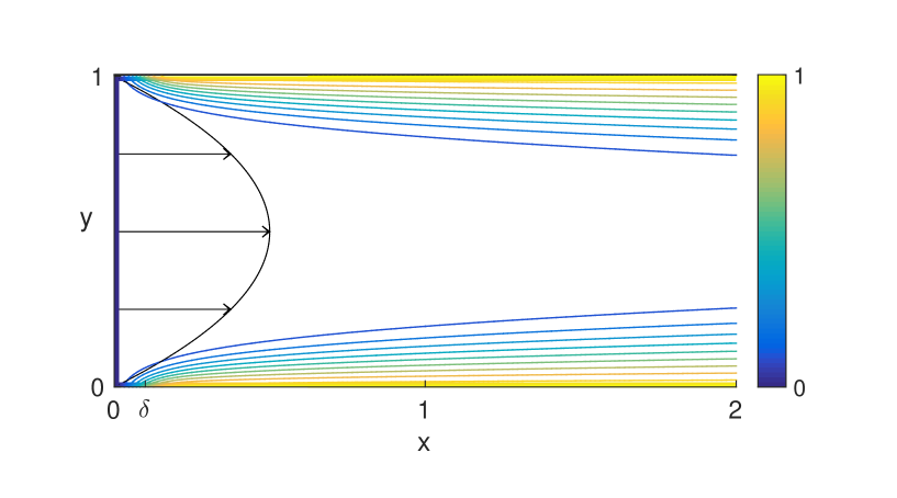
Figure 1: Temperature contours for parabolic (Poiseuille) flow through a channel with height 1 and length 2. At the upstream boundary the fluid temperature is zero. On the top and bottom walls the fluid temperature is $1-e^{-x^{2}/\delta^{2}}$ with the smoothing parameter $\delta$ set to 0.1. The flow is purely horizontal with velocity profile $u(y)=512\sqrt{6}(y-y^{2})$, corresponding to dimensionless parameter values $Pe=1024$ and $L=2$.

We consider steady incompressible 2D fluid flows $\mathbf{u}=(u(x,y),v(x,y))$ in a channel of height $H$ and length $L_{0}$ occupying $0\leq x\leq L_{0}$, $0\leq y\leq H$ (see Figure 1). The fluid temperature field $T(x,y)$ solves the steady advection-diffusion equation

$$\mathbf{u}\cdot\nabla T-\kappa\Delta T =0,$$ (1)

with $\kappa$ the thermal diffusivity of the fluid, equal to $k/\rho c_{p}$, where $k$ is the thermal conductivity, $\rho$ the fluid density and $c_{p}$ the specific heat capacity at constant pressure. At the inflow boundary, $x=0$, cold fluid enters with temperature $T=0$. At the outflow boundary, $x=L_{0}$, we use an outflow boundary condition $\partial_{x}T=0$, so the fluid temperature maintains its value from slightly upstream of the boundary. On the top and bottom walls, $y=0$ and $H$, the temperature is set to $T=1-e^{\displaystyle-x^{2}/\delta^{2}}$, where $\delta$ is a small smoothing parameter. The temperature is nearly unity over most of the walls. We use $\delta$ to avoid a temperature singularity where the walls meet the upstream boundary, and ease the numerical resolution requirements. We work in the regime $\delta\ll H,\delta\ll L_{0}$, and find little dependence of the solutions on $\delta$ in this limit.

The entering cold fluid heats up as it flows past the walls, so the exiting fluid has a higher temperature. Integrating (1) over the channel and using the divergence theorem, we have

$$\int T\mathbf{u}\cdot\mathbf{n}ds=\int\kappa\partial_{n}Tds.$$ (2)

where the integrals are over the entire boundary (top, bottom, upstream, and downstream). We assume no-slip conditions on the top and bottom walls ($\mathbf{u}=0$), leaving only the upstream and downstream sides to contribute to the left side of (2). This term gives the net advection of heat out of the channel (divided by $\rho c_{p}$). The right side gives the net heat flux into the channel by conduction from the boundaries (divided by $\rho c_{p}$). The downstream boundary does not contribute due to the outflow condition $\partial_{x}T=0$. For flows with typical speed $\gg\kappa/H_{0}$ (the usual case in applications), conduction through the upstream boundary is slight and most of the heat flux is from the top and bottom walls.

III Viscous Energy Dissipation Constraint

The problem we consider is to find an incompressible fluid flow $\mathbf{u}$ that maximizes the (steady) rate of heat flux out of the hot walls,

$$\int_{0}^{L_{0}}k\,\left(\partial_{y}T|_{y=H}-\partial_{y}T|_{y=0}\right)dx,$$ (3)

for a given rate of viscous dissipation per unit width in the out-of-plane direction,

$$\dot{E}=2\mu W\iint e_{ij}e_{ij}dA=\mu W\iint(\Delta\psi)^{2}dA.$$ (4)

Here $\mu$ is viscosity, $W$ is the out-of-plane width (along which the flow and temperature are uniform), and $e_{ij}=(\nabla\mathbf{u}+\nabla\mathbf{u}^{T})/2$ is the symmetric part of the rate-of-strain tensor. The last term in (4) involves the stream function $\psi$, which is defined for an incompressible 2D flow by $\mathbf{u}=-\nabla^{\perp}\psi=(\partial_{y}\psi,-\partial_{x}\psi)$. The second equality in (4) is derived in lamb1932hydrodynamics (article 329) and holds for certain boundary conditions including those we will use here (we will have $v\equiv 0$ on the boundaries, which is sufficient for (4)).

A (sufficiently smooth) incompressible flow solves the Navier-Stokes equations

$$\rho\frac{D\mathbf{u}}{Dt}=-\nabla p+\mu\Delta\mathbf{u}+\mathbf{f}\quad;\quad\nabla\cdot\mathbf{u}=0,$$ (5)

for a suitable forcing term $\mathbf{f}$, which represents a force per unit volume applied over the fluid domain. If $\mathbf{f}$ takes the form of a $\delta$-distribution along a rigid or deforming no-slip surface, it represents the surface stress such boundaries apply to the flow, as in the immersed boundary formulation Griffith07 ; shoele2014computational . Much previous work has studied the enhancement of heat transfer by vortices shed from rigid or flexible bodies in the flow gee1980forced ; tsia1999measurements ; promvonge2010enhanced ; shoele2014computational ; rips2017efficient . A smooth $\mathbf{f}$ represents a distribution of forces spread over the flow domain, and can approximate those applied within localized regions such as the no-slip surfaces of vortex-generating obstacles, or powered fans.

Taking the dot product on both sides of the first equation in (5) with $\mathbf{u}$ and integrating over the channel, we obtain the energy balance equation after some manipulations durst2008fluid :

$$\frac{d}{dt}\iint\frac{\rho|\mathbf{u}|^{2}}{2}dA+\int_{0}^{H}\frac{\rho|\mathbf{u}|^{2}}{2}u\Big{|}^{x=L_{0}}_{x=0}dy+\dot{E}/W=\int_{0}^{H}pu\Big{|}^{x=L_{0}}_{x=0}dy+\iint\mathbf{f}\cdot\mathbf{u}dA.$$ (6)

We will assume steady flow, which is the same at the inflow and outflow boundaries, so (6) becomes

$$\dot{E}/W=\int_{0}^{H}pu\Big{|}^{x=L_{0}}_{x=0}dy+\iint\mathbf{f}\cdot\mathbf{u}dA.$$ (7)

The rate of work done by the volume distribution of forces $\mathbf{f}$ and the pressure at the upstream and downstream boundaries equals the rate of viscous dissipation (per unit width). Previous works gee1980forced ; tsia1999measurements ; promvonge2010enhanced ; shoele2014computational ; rips2017efficient considered flows with the cost defined as the “pumping power,” the first term on the right side of (7). Our definition of cost is the rate of viscous dissipation, which by (7) is equal to both terms on the right side of (7): pressure at the boundaries and volume forces in the interior. Thus our cost is the same as the “pumping power,” generalized to include volume forces. In previous work the volume forces are actually surface forces applied by fixed or flexible elastic obstacles in the channel. These do no net time-averaged work on the flow since $\mathbf{u}=0$ on the fixed bodies, and the stored elastic energy remains bounded at large times for moving flexible bodies. Our optimization formulation allows an arbitrary body force distribution $\mathbf{f}$, though we restrict to 2D steady flows and forcing in this work to begin with the simplest case. In Appendix A we describe how to compute $\mathbf{f}$ and $p$ from (5), given $\mathbf{u}$, as the solution to coupled Poisson equations.

IV Dimensionless equations and boundary conditions

We nondimensionalize lengths by the channel height $H$ and time by a diffusion time scale $H^{2}/\kappa$. We have already nondimensionalized temperature by the temperature of the hot boundary (for $x\gg\delta$), relative to the temperature of the entering fluid. Having chosen scales for length, time and temperature, we need to choose a typical mass scale to nondimensionalize (3). Since mass enters the thermal conductivity, for simplicity we instead chose a thermal conductivity scale to be that of the fluid.

We maximize the dimensionless form of (3),

$$Q=\int_{0}^{L}\left(\partial_{y}T|_{y=1}-\partial_{y}T|_{y=0}\right)dx$$ (8)

where $L=L_{0}/H$, over $T$ satisfying the dimensionless form of (1),

$$\partial_{y}\psi\partial_{x}T-\partial_{x}\psi\partial_{y}T-\Delta T =0,$$ (9)

for a flow $\psi(x,y)$ with rate of viscous dissipation fixed by a constant $Pe^{2}$,

$$\int_{0}^{1}\int_{0}^{L}(\Delta\psi)^{2}dxdy=Pe^{2}=\dot{E}H^{2}/W\mu\kappa^{2}.$$ (10)

Here $W$ is the width of the channel in the out-of-plane direction. The optimal flow $\psi$ is found by setting to zero the variations of the Lagrangian

$$\mathcal{L}=\int_{0}^{L}\left(\partial_{y}T|_{y=1}-\partial_{y}T|_{y=0}\right)dx+\int_{0}^{1}\int_{0}^{L}m(x,y)\left(-\nabla^{\perp}\psi\cdot\nabla T-\Delta T\right)dxdy+\lambda\left(\int_{0}^{1}\int_{0}^{L}(\Delta\psi)^{2}dxdy-Pe^{2}\right).$$ (11)

with respect to $T$, $\psi$, and Lagrange multipliers $m$ and $\lambda$ that enforce (9) and (10) respectively. The area integrals are over the fluid domain, the rectangle in figure 1. Taking the variations and integrating by parts, we obtain the following system of three nonlinear partial differential equations (PDEs) plus one integral constraint. We supplement the PDEs with the listed boundary conditions:

PDE/Constraint Upstream BCs Top BCs Bottom BCs Downstream BCs

$$0=\frac{\delta\mathcal{L}}{\delta m}=-\nabla^{\perp}\psi\cdot\nabla T-\Delta T T=0\; T=1-e^{-\displaystyle\frac{x^{2}}{\delta^{2}}} T=1-e^{-\displaystyle\frac{x^{2}}{\delta^{2}}} \partial_{x}T=0$$ (12)

$$0=\frac{\delta\mathcal{L}}{\delta T}=\nabla^{\perp}\psi\cdot\nabla m-\Delta m m=0\; m=1 m=1 \partial_{x}m+m\partial_{y}\psi=0$$ (13)

$$0=\frac{\delta\mathcal{L}}{\delta\psi}=-c\nabla^{\perp}T\cdot\nabla m-2\Delta^{2}\psi \psi=\psi_{top}(3y^{2}-2y^{3}), \psi=\psi_{top}, \psi=0, \psi=\psi_{top}(3y^{2}-2y^{3}),$$ (14)

$$\partial_{x}\psi=0 \partial_{y}\psi=0 \partial_{y}\psi=0 \partial_{x}\psi=0$$ (15)

$$0=\frac{\delta\mathcal{L}}{\delta\lambda}=\int_{0}^{1}\int_{0}^{L}(\Delta\psi)^{2}dxdy-Pe^{2}.$$ (16)

The boundary conditions for $T$ in (12), the usual ones for flow through a heated channel shoele2014computational , have already been discussed.

The top and bottom boundary conditions for $\psi$ in (14) and (15) correspond to the no-slip condition on the channel walls, with a net mass flux $\psi_{top}$ (an additional variable to be discussed) through the channel. At the upstream and downstream boundaries we set $\psi$ so the flow has a parabolic velocity profile (Poiseuille flow) with the same mass flux $\psi_{top}$ (as required for incompressible flow). If instead any incompressible flow is allowed at these boundaries, then the “natural” boundary conditions are used. These are given by setting the boundary terms (not shown) in $\delta\mathcal{L}/\delta\psi$ to zero. These terms involve $\Delta\psi$ and $\partial_{x}\Delta\psi$ together with lower order derivatives of $m$ and $T$. These boundary conditions are not well-posed for the biharmonic operator, as discussed in hsiao2008boundary , and lead to nonconvergence of the finite difference scheme we use. Furthermore, they do not impose inflow and outflow ($u=\partial_{y}\psi>0$) at the corresponding boundaries, so they may violate the basic physical assumptions of the model. It is possible to use other boundary conditions at the upstream and downstream boundaries, but an advantage of imposing Poiseuille flow at these boundaries is that they allow us to generate optimal solutions by continuation from a simple starting solution, Poiseuille flow itself. In (14) we have inserted $c\equiv 1/\lambda$. For the starting Poiseuille flow solution, $\lambda=\pm\infty$ while $c=0$, so $c$ is more convenient for computations.

The boundary conditions for $m$, given in (13), make the boundary terms (not shown) in $\delta\mathcal{L}/\delta m$ equal to zero.

V Solutions

Poiseuille flow,

$$\psi_{Pois}(x,y)\equiv\psi_{top}(3y^{2}-2y^{3}),$$ (17)

with a certain value of $\psi_{top}$ and certain choices $\{\bar{T},\bar{m},\bar{c}\}$ for $\{T,m,c\}$, respectively, gives a convenient starting solution to equations (12)–(16). We can see that it is a solution by first plugging $\psi_{Pois}$ into equation (16). We find that when $\psi_{top}=\bar{\psi}_{top}\equiv Pe/\sqrt{12L}$, the corresponding $\psi_{Pois}$, which we call $\bar{\psi}_{Pois}$, satisfies the equation. Second, $\bar{\psi}_{Pois}$ is a biharmonic function, and it satisfies (14)–(15) with $c=\bar{c}\equiv 0$ and $\psi_{top}=\bar{\psi}_{top}$. Plugging $\bar{\psi}_{Pois}$ into (12) and (13) and solving, we then obtain $\bar{T}$ and $\bar{m}$, respectively.

In fact, this starting solution is the unique solution to (12)–(16) when $\psi_{top}=Pe/\sqrt{12L}$. We can show this by writing any solution as

$$\psi=\psi_{Pois}+\tilde{\psi}.$$ (18)

We will use this decomposition even when $\psi_{top}\neq Pe/\sqrt{12L}$, to write solutions in terms of $\tilde{\psi}$. Plugging (18) into (16), we find after integrating by parts and using homogeneous boundary conditions for $\tilde{\psi}$ that

$$12L\psi_{top}^{2}+\int_{0}^{1}\int_{0}^{L}(\Delta\tilde{\psi})^{2}dxdy=Pe^{2}.$$ (19)

If $\psi_{top}=Pe/\sqrt{12L}$, then $\Delta\tilde{\psi}\equiv 0$, and again using the homogeneous boundary conditions for $\tilde{\psi}$ implies $\tilde{\psi}\equiv 0$.

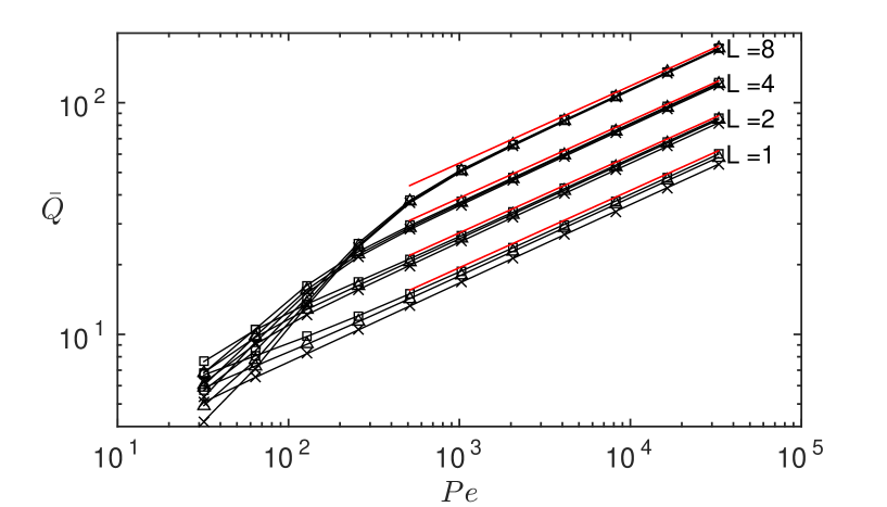
Figure 2: Heat transfer for Poiseuille flow in a channel, denoted $\bar{Q}$, at various $Pe$, $L$ = 1, 2, 4, and 8 (labeled), and $\delta$ = 0.05 (squares), 0.1 (triangles), and 0.2 (crosses). The red lines show, for each $L$, the leading-order term in $Q$ from the similarity solution of worsoe1967heat (based on that of leveque1928laws and reported on page 173 of shah2014laminar ).

The benchmark solution at a given $Pe$ is $\bar{\psi}_{Pois}$, so we first show how $Q$ for this solution, denoted $\bar{Q}$, varies with parameters before giving the results for other optima. Figure 2 plots $\bar{Q}$ versus $Pe$ for four different values of $L$. For each $L$, we have a cluster of three lines (labeled by the value of $L$) giving $Q$ values at three $\delta$, 0.05, 0.1, and 0.2, to show the effect of this smoothing parameter. We find a slight increase in the heat transferred as $\delta\to 0$. The red line gives the leading term for the similarity solution of worsoe1967heat (from shah2014laminar ), which corresponds to the case $\delta=0$. Here the temperature profile is a function of a similarity variable

$$\eta\equiv yPe^{1/3}/x^{1/3}L^{1/6}$$ (20)

near the bottom wall (with a symmetrically reflected boundary layer at the top wall, taking $1-y$ in place of $y$). The combination $Pe^{1/3}/L^{1/6}$ is essentially flow speed to the 1/3-power, since for Poiseuille flow $\bar{\psi}_{top}\equiv Pe/\sqrt{12L}$. The width of the boundary layer in the $y$ direction at a given $x$ scales as $Pe^{-1/3}L^{1/6}$ and the temperature contours in Figure 1 grow like a cube root of $x$ moving downstream. The total heat transferred for the similarity solution is given by worsoe1967heat , and in terms of our parameters ($Pe$ and $L$), it is $\bar{Q}\sim 1.85(4/3)^{1/6}Pe^{1/3}L^{1/2}$, shown by the red lines in Figure 2. At smaller $Pe$ (slower flows) and larger $L$ (longer channels), the values deviate from the red lines because the thermal boundary layers on the top and bottom (shown in Figure 1) are large enough to intersect within the channel, and the solutions are no longer well-approximated by the similarity solution.

Our procedure for generating optimal flows is then the following continuation scheme. For each $Pe$, we start with $\psi_{top}=\bar{\psi}_{top}=Pe/\sqrt{12L}$ and the unique optimum $\{\bar{T},\bar{m},\bar{\psi}_{Pois},\bar{c}\}$. We then decrease $\psi_{top}$ gradually, and compute the solution to (12)–(16) using Newton’s method with the solution at the previous value of $\psi_{top}$ as an initial guess. The best among these solutions is not necessarily a global optimum. For example, there could be optima that are not smoothly continued from the starting solution. However, from the computed solutions we do obtain a local optimum which provides a lower bound on the performance of a global optimum. Furthermore, because there is a unique starting solution, we can characterize the set of possible optima in the vicinity of the starting solution (discussed more fully in the next section, VI).

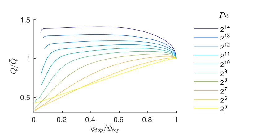
Figure 3: Values of heat transferred $Q$, relative to that of the starting Poiseuille solution $\bar{Q}$, for optimal flows with $Pe$ ranging from $2^{5}$ to $2^{14}$ and $\psi_{top}/\bar{\psi}_{top}$ ranging from 1 down to 0-0.1 (where our Newton’s method stops converging). The channel length $L$ = 2.

In Figure 3 we show the heat transferred for the optimal solutions as the continuation parameter $\psi_{top}/\bar{\psi}_{top}$ ranges from 1 down to 0–0.1 (where our Newton’s method stops converging).

For the smallest $Pe$ = 32 the optimum occurs for $\psi_{top}/\bar{\psi}_{top}$ very close to 1, so Poiseuille flow is almost optimal. As the flow becomes even slower ($u\sim Pe/\sqrt{L}\lesssim 1$) or the channel longer (larger $L$), the temperature is nearly its maximum (unity) all along the outflow boundary, so the heat flux out of this boundary is almost the same as the net flow rate:

$$\int_{0}^{1}T\mathbf{u}\cdot\mathbf{n}|_{x=L}\,dy\approx\int_{0}^{1}1\,\mathbf{u}\cdot\mathbf{n}|_{x=L}\,dy=\psi_{top}.$$ (21)

Since Poiseuille flow maximizes the flow rate at a given $Pe$, it is not surprising that it is nearly optimal. More precisely, if we consider the similarity solution for temperature in a Poiseuille flow mentioned above, the temperature is close to unity throughout the outflow boundary if the boundary layer extends well past the middle of the channel ($y=1/2$) at $x=L$, which means the similarity variable is $\ll 1$ there: $1\gg\eta\equiv yPe^{1/3}/x^{1/3}L^{1/6}\sim Pe^{1/3}/L^{1/2}$ at $y=1/2$ and $x=L$. In the example above, $Pe=32$ and $L=2$, so $Pe^{1/3}/L^{1/2}=2.2$ is not yet in the regime $Pe^{1/3}/L^{1/2}\ll 1$, but is close to it. In this regime, the optimal flow is very close to Poiseuille flow. As $\bar{\psi}_{top}\equiv Pe/\sqrt{12L}$ approaches zero, the upstream and downstream temperature boundary conditions are no longer physically realistic since they assume strong advection ($Pe/\sqrt{L}\gg 1$).

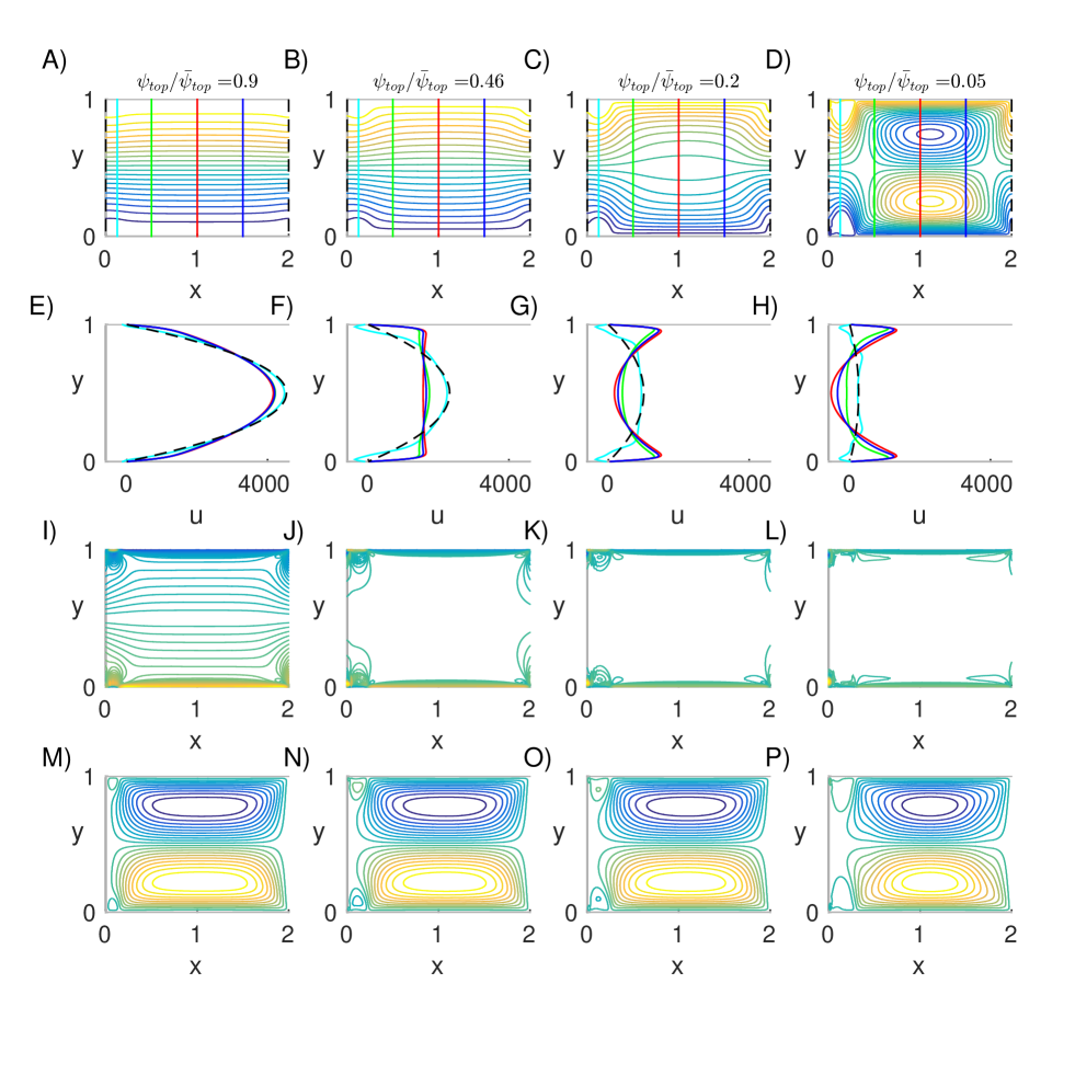
Figure 4: Optimal flows for $Pe=2^{14}$ and four different values of $\psi_{top}/\bar{\psi}_{top}$: 0.9 (first column), 0.46 (second column), 0.2 (third column), and 0.05 (fourth column). The values of $Q$ are: 84.4 (first column), 95.2 (second column), 94.1 (third column), and 91.3 (fourth column). The values of $\tilde{\psi}_{max}$ are (I) 69.5, (J) 141.2, (K) 156.7, and (L) 149.3.

As we move from $Pe=32$ to larger $Pe$ in figure 3, we see that the $Q$-maximizing flow occurs at a decreasing value of $\psi_{top}/\bar{\psi}_{top}$, and moves further from Poiseuille flow. Also, the heat transfer improvement $Q/\bar{Q}$ increases with increasing $Pe$. To understand the corresponding physics, we focus on the highest $Pe$ shown in figure 3: $2^{14}$. At this $Pe$ we plot the flows at four values of $\psi_{top}/\bar{\psi}_{top}$, in the four columns on figure 4. Moving from the first column to the fourth column, we move away from the Poiseuille flow optimum by decreasing the flux $\psi_{top}/\bar{\psi}_{top}$ to 0.9, 0.46, 0.2, and 0.05. The different rows plot different flow quantities for each optimum. The first row shows streamlines for the total flow, $\psi$. The second row shows the horizontal velocity profile along six cross-sections marked in the first row (with corresponding colors). The third row shows contours of the vorticity fields. The fourth row shows streamlines for $\tilde{\psi}$, the total flow minus the Poiseuille flow component, defined in (18).

In the first column, the flow is close to the initial Poiseuille flow optimum. The streamlines (A) are nearly unidirectional, with bending slightly towards the wall at the inflow and away from the wall at the outflow. The flow profiles $u(y)$ (E) are prescribed as Poiseuille flow (black dashed lines) at the inflow and outflow boundaries. The profiles at 1/4 (green), 1/2 (red), and 3/4 (blue) of the channel length are nearly identical and are perturbations of the Poiseuille inflow and outflow, with a slight weakening of the parabolic flow in the center and a strengthening of the flow near the walls. The vorticity (I) has a nearly uniform gradient (as for Poiseuille flow) around $y=1/2$, but with a sharp increase near the boundaries. The $\tilde{\psi}$-component (M) shows two large vortices, equal and opposite, with downstream flow near the walls and upstream flow near $y=1/2$. A smaller pair of oppositely-signed vortices is located on the wall near the inflow boundary, where the wall temperature changes from 0 to 1.

The second column shows the flow that maximizes $Q$ over all $\psi_{top}/\bar{\psi}_{top}$ at this $Pe$. Here $Q$ is 41% higher than that of the initial Poiseuille flow, while the net flow through the channel is reduced to 46% of its initial value. Panel B shows streamlines that are nearly unidirectional as in A, but spread towards the walls. The spacing between the streamlines is nearly uniform, indicating a nearly uniform flow. This is shown clearly in panel F, where the green, red, and blue velocity profiles are all nearly uniform except for sharp boundary layers near the walls. The vorticity is now almost entirely at the walls (panel J), with additional vorticity near the inflow and outflow boundaries at the walls. The $\tilde{\psi}$-component (N) has a spatial distribution similar to that in first column, with somewhat larger vortices at the corners near the inflow boundary. In the third column, the net flow is only 0.2 times its initial value, but $Q$ is still 99% that of the second column. The flow is now very nonuniform near $y=1/2$ (panel C). Panel G shows that it resembles a backward facing parabolic profile. Otherwise, the features are similar to those in the second column. In the fourth column, the net flow is reduced to 0.05 its initial value. The flow divides into regions of downstream flow near the walls and two closed eddies with upstream flow in the center of the channel near $y=1/2$ and $1/2<x<3/2$. However, the flow profiles (H) are not so different from the third column (G). Again we have backward facing parabolic profiles for $1/2<x<3/2$, which cross zero, corresponding to upstream flow. Surprisingly, the $\tilde{\psi}$-component (P) is not much different now, and $Q$ is almost (96%) that of the optimum (second column).

We would like to explain some of the key features of the optimal flows, and in particular, determine for these flows how $Q$ scales with $Pe$ and $L$. We will use a combination of approximations, computations, and asymptotics. First we will give a simple intuitive explanation for what happens as $\psi_{top}/\bar{\psi}_{top}$ is decreased from 1 at a given $Pe$. For a Poiseuille flow with large $Pe$, the temperature is large near the walls and essentially zero elsewhere (as in figure 1, except that in figure 4 $Pe$ is larger ($2^{14}$), so the temperature boundary layer is a factor of $2^{4/3}\approx 2.5$ thinner in Poiseuille flow). To move more heat out of the channel, it is advantageous to increase the downstream flow where the temperature is nonzero (near the walls), which means having a steeper velocity gradient near the no-slip walls. To keep the total enstrophy ($Pe^{2}$) constant, enstrophy is then depleted from the center of the channel (near $y=1/2$), slowing the downstream flow there. Since the temperature is zero there for all $x$, this depletion does not decrease the heat flux through the channel. The net effect of moving enstrophy from the channel center to the walls is to increase the heat flux out. The second column of figure 4 is optimal because the flow is uniform in the center of the channel, so no enstrophy is spent there. All of the enstrophy is in the boundary layers near the walls, giving the maximum possible downstream flow there. In the third and fourth columns, with much smaller net flux prescribed, some enstrophy is put back into the center of the channel, which takes enstrophy from the wall boundary layers and therefore slows them down. However, the velocity gradient is still large enough near the walls to transfer nearly the optimal amount of heat out of the channel. There may be some additional compensating effects for the slower flows, in that there is more time to mix the hotter fluid near the wall with colder fluid away from the wall before the fluid leaves the channel, as proposed by gerty2008fluidic ; hidalgo2010heat ; shoele2014computational ; jha2015small . However, unlike the heat transfer enhancement strategies using vortex shedding, here the optimal flow (second column) is mainly in the $x$-direction, and does not contain a sequence of coherent vortices. The vortices near the inflow boundary are the only occurrence of discrete vortices in the flow.

In the last paragraph we have given the physical intuition for the optimal flow structure. In the next section, we analyze the mathematical structure and asymptotic scalings using a decoupled approximation for the optimal flows. Readers who are less interested in the mathematical details may wish to skip to the following section, which explains the asymptotic scalings for the fully coupled system using a unidirectional flow approximation, and gives physical interpretations.

VI Decoupled approximation

In order to determine how the heat transfer $Q$ scales with $Pe$ and $L$, we use the method of successive approximations lin1988mathematics for the nonlinear equations (12)–(16). When $\psi_{top}$ is close to $\bar{\psi}_{top}$, $\psi\approx\bar{\psi}_{Pois}\approx\psi_{Pois}$, $\|\tilde{\psi}\|\ll\|\psi_{Pois}\|$, $T\approx\bar{T}$, and $m\approx\bar{m}$. This motivates the following approximation to (12)–(16). First we write the $\psi$ equations (14)–(15) in terms of $\tilde{\psi}$ defined in (18) (no approximation yet). Then we approximate $T$ and $m$ in (14)–(15) by their values in the initial Poiseuille solution, $\bar{T}$ and $\bar{m}$, respectively. Then the coupling from $\bar{m}$ and $\bar{T}$ to $\tilde{\psi}$ is one-way:

PDE/Constraint Upstream BCs Top BCs Bottom BCs Downstream BCs

$$0=-\nabla^{\perp}\bar{\psi}_{Pois}\cdot\nabla\bar{T}-\Delta\bar{T} \bar{T}=0\; \bar{T}=1-e^{-\displaystyle\frac{x^{2}}{\delta^{2}}} \bar{T}=1-e^{-\displaystyle\frac{x^{2}}{\delta^{2}}} \partial_{x}\bar{T}=0$$ (22)

$$0=\nabla^{\perp}\bar{\psi}_{Pois}\cdot\nabla\bar{m}-\Delta\bar{m} \bar{m}=0\; \bar{m}=1 \bar{m}=1 \partial_{x}\bar{m}+\bar{m}\partial_{y}\bar{\psi}_{Pois}=0$$ (23)

$$0=-c_{1}\nabla^{\perp}\bar{T}\cdot\nabla\bar{m}-2\Delta^{2}\tilde{\psi}_{1} \tilde{\psi}_{1}=0, \tilde{\psi}_{1}=0, \tilde{\psi}_{1}=0, \tilde{\psi}_{1}=0,$$ (24)

$$\partial_{x}\tilde{\psi}_{1}=0 \partial_{y}\tilde{\psi}_{1}=0 \partial_{y}\tilde{\psi}_{1}=0 \partial_{x}\tilde{\psi}_{1}=0$$ (25)

$$0=\int_{0}^{1}\int_{0}^{L}(\Delta\tilde{\psi}_{1})^{2}dxdy+12L\psi_{top}^{2}-Pe^{2}.$$ (26)

$$0=-\nabla^{\perp}\left({\psi}_{Pois}+\tilde{\psi}_{1}\right)\cdot\nabla T_{1}-\Delta T_{1} T_{1}=0\; T_{1}=1-e^{-\displaystyle\frac{x^{2}}{\delta^{2}}} T_{1}=1-e^{-\displaystyle\frac{x^{2}}{\delta^{2}}} \partial_{x}T_{1}=0$$ (27)

Note that $\tilde{\psi}_{1}$ in (24)–(25) is an approximation to $\tilde{\psi}$ (since $\bar{T}$ and $\bar{m}$ are computed using $\bar{\psi}_{Pois}$ instead of $\psi=\psi_{Pois}+\tilde{\psi}$). Equation (27) computes the temperature field $T_{1}$ for this approximation to the optimal flow, from which we compute the heat transferred, $Q_{1}$.

In (24) $c_{1}$ is an approximation to $c$, computed by plugging $\tilde{\psi}_{1}$ from (24) into (26):

$$c_{1}=\pm 2\sqrt{Pe^{2}-12L\psi_{top}^{2}}\Bigg{/}\sqrt{\int_{0}^{1}\int_{0}^{L}\left(\Delta^{-1}(\nabla^{\perp}\bar{T}\cdot\nabla\bar{m})\right)^{2}dxdy}.$$ (28)

Due to the $\pm$ in (28), there are two branches of approximate optimal flows

$$\tilde{\psi}_{1}=\mp\Delta^{-2}(\nabla^{\perp}\bar{T}\cdot\nabla\bar{m})\sqrt{Pe^{2}-12L\psi_{top}^{2}}\Bigg{/}\sqrt{\int_{0}^{1}\int_{0}^{L}\left(\Delta^{-1}(\nabla^{\perp}\bar{T}\cdot\nabla\bar{m})\right)^{2}dxdy}$$ (29)

leading away from the starting optimum. The negative sign gives a local minimizer of heat transferred $Q_{1}$ and the positive sign gives a local maximizer, so this is the branch we compute. The approximation we have made should be good for $\psi_{top}$ close to $\bar{\psi}_{top}$ but the fourth row of figure 4 gives us hope that it works well for a much larger range of $\psi_{top}$, because there is relatively little change in the spatial distribution of $\tilde{\psi}$ for $0.05\leq\psi_{top}/\bar{\psi}_{top}\leq 0.9$. As $\psi_{top}$ varies, $\tilde{\psi}_{1}$ in (29) has a fixed spatial distribution, scaled by different constants $\sqrt{Pe^{2}-12L\psi_{top}^{2}}$.

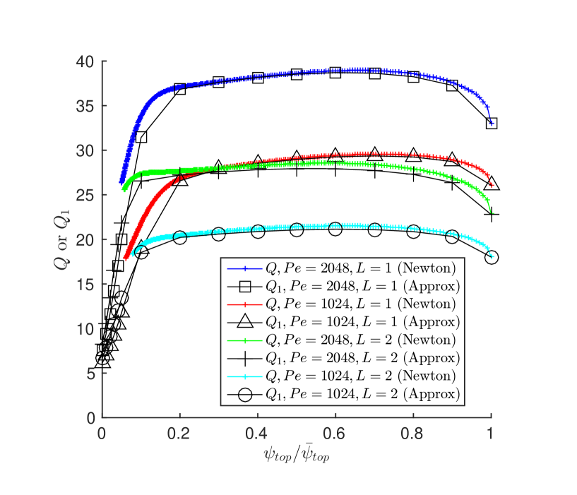
Figure 5: Comparison of the heat transferred by the optimal flows ($Q$, colored lines) computed by solving the nonlinear equations (12)–(16) with that transferred by the approximate optimal flows ($Q_{1}$, black lines), computed by solving (22)–(27). Two channel lengths ($L=1,2$) and two values of $Pe$ (1024 and 2048) are used.

In figure 5 we compare the heat transferred by the approximate optimal flow $\psi_{1}\equiv{\psi}_{Pois}+\tilde{\psi}_{1}$ (using (27)) with that from $\psi={\psi}_{Pois}+\tilde{\psi}$, the flow solution to the full nonlinear equations (12)–(16). We use two channel lengths $L=1,2$ and two values of $Pe$, 1024 and 2048. For each of the four parameter combinations we plot the heat transferred versus $\psi_{top}/\bar{\psi}_{top}$ for the nonlinear solution ($Q$, colored lines) and the approximation ($Q_{1}$, black lines). The agreement is remarkably good over a broad range, $0.1\leq\psi_{top}/\bar{\psi}_{top}\leq 1$. In the approximate flow equation (24) we used $\bar{T}$, the temperature due to the starting Poiseuille flow $\bar{\psi}_{Pois}$, instead of $T$, the temperature due to the actual flows $\psi$, which are quite different from Poiseuille flow, especially for smaller $\psi_{top}/\bar{\psi}_{top}$, as shown by the first row of figure 4.

Although $\bar{\psi}_{Pois}$ is quite different from $\psi$, it turns out that $\bar{T}$ is similar to $T$. The reason, briefly, is that $\bar{T}$ and $T$ both transition from 1 to 0 over thin boundary layers near the wall, so they are only affected by the flows there. In the boundary layers, $\psi$ and $\bar{\psi}_{Pois}$ both have sharp linear flow gradients near the wall, with that from $\psi$ somewhat sharper. The differences between $\psi$ and $\bar{\psi}_{Pois}$ outside the boundary layers have little effect on the temperature field because it is nearly zero there.

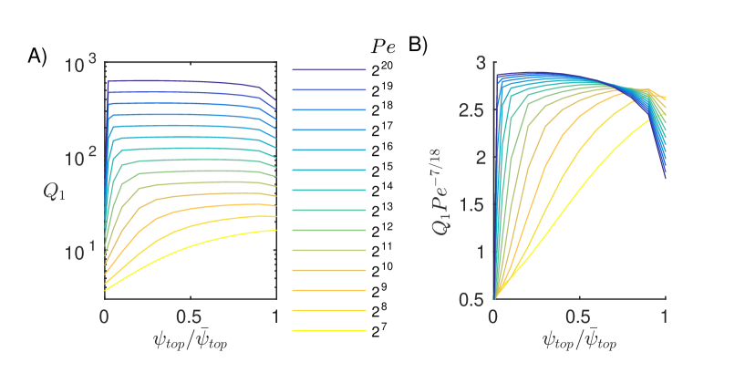
Figure 6: Heat transferred ($Q_{1}$) by the approximate optimal flows. A) $Q_{1}$ versus $\psi_{top}/\bar{\psi}_{top}$ at several values of $Pe$ (listed to the right). B) $Q_{1}$ rescaled by $Pe^{7/18}$.

As $Pe$ grows, it becomes difficult to obtain convergence with Newton’s method for our finite-difference discretization of (12)–(16). The Jacobian matrix contains a biharmonic operator, for which the condition number scales as grid spacing to the $-4$ power. At large $Pe$, a fine grid is needed near the boundaries to resolve the boundary layers in $T$, $m$, and $\psi$. To obtain the asymptotic scaling of $Q$ with $Pe$ at larger $Pe$ than the maximum value in figure 3 ($=2^{14}$), we proceed with calculations of the approximate optimal flow $\psi_{1}\equiv{\psi}_{Pois}+\tilde{\psi}_{1}$ and the resulting temperature field $T_{1}$ in (24), (25), and (27), respectively. These can be calculated using direct solvers for the linear systems in (22)–(27), so we avoid Newton’s method and associated convergence issues. Although the approximate flows do not achieve the optimal heat transfer, their heat transfer is close to that of the optimal flows in figure 5, and they show us how to obtain the right scalings for the optimal flows.

In figure 6A we plot $Q_{1}$, the heat transferred by the approximate optimal flows $\psi_{1}$, up to $Pe=2^{20}$, and across the full range $0\leq\psi_{top}/\bar{\psi}_{top}\leq 1$. When $\psi_{top}/\bar{\psi}_{top}=1$ the solution is $\bar{\psi}_{Pois}$ with heat transfer $\bar{Q}\sim Pe^{1/3}$. The maximum of $Q_{1}$ over $\psi_{top}/\bar{\psi}_{top}$ exceeds $\bar{Q}$, and the difference grows with $Pe$. We will subsequently argue that max($Q_{1}$) $\sim Pe^{7/18}$. In panel B we plot $Q_{1}$ divided by $Pe^{7/18}$ and see an approximate collapse of the maxima of the curves. The slight improvement of 7/18 over 1/3 is due to reconfiguring the flow as $Pe$ increases rather than simply speeding up a given (Poiseuille) flow profile.

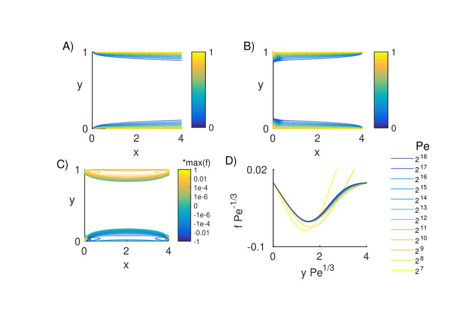
Figure 7: Plots of the components of the source terms for the approximate optimal flow, $\tilde{\psi}_{1}$ in (24). A: Contours of $\bar{T}$ at $Pe=2^{15}$, $L=4$, and $\delta=0.05$. B: Contours of $\bar{m}$ at the same parameters. C: Contours of $f\equiv\partial_{x}\bar{T}\partial_{y}\bar{m}-\partial_{y}\bar{T}\partial_{x}\bar{m}$ at the same parameters. D: Profiles of $f$ along the channel midline at $x=L/2=2$, at various $Pe$, rescaled near $y=0$ to show the asymptotic behavior.

To understand how a $Pe^{7/18}$ scaling arises from the equations, we plot in figure 7 the contributions to the “source term” in the biharmonic equation for $\tilde{\psi}_{1}$ (24). In panel A, we plot the contours of $\bar{T}$ at $Pe=2^{15}$ and $L=4$, showing the same kind of Poiseuille-flow temperature boundary layer as in figure 1, but narrower at this larger $Pe$. Panel B shows the corresponding $\bar{m}$. Since $\bar{m}$ solves the backward advection diffusion equation (23), we have a profile which is almost that of $\bar{T}$ reflected in the $x$-midpoint of the channel. The boundary conditions in (23) are somewhat different than in (22). Along the walls $\bar{m}=1$, close to the values of $\bar{T}$ since $\delta$ is small (0.05 here). At $x=L$, $\partial_{x}\bar{m}+\bar{m}\partial_{y}\bar{\psi}_{Pois}=0$, and since $\partial_{x}\bar{m}$ is exponentially small outside the boundary layer, but $\partial_{y}\bar{\psi}_{Pois}$ is $O(Pe)\gg 1$, $\bar{m}$ is also exponentially small outside the boundary layer. At $x=0$, $\bar{m}=0$, but since we have strong advection in the $-x$ direction, this only affects the solution in a thin layer near $x=0$, too thin to be visible in panel B. In panel C we plot on a logarithmic scale contours of $f\equiv\partial_{x}\bar{T}\partial_{y}\bar{m}-\partial_{y}\bar{T}\partial_{x}\bar{m}$, the source term for $\tilde{\psi}_{1}$ in (24), up to a constant ($c_{1}$). Because $\bar{T}$ and $\bar{m}$ are essentially constant (zero) outside a distance $\sim Pe^{-1/3}$ from the walls, so is the source term. Using the approximate similarity solutions $\bar{T}=g(\eta)$, $\bar{m}=g(\tilde{\eta})$, with $\eta$ in (20) and

$$\tilde{\eta}\equiv yPe^{1/3}/(L-x)^{1/3}L^{1/6},$$ (30)

we have

$$f=-\frac{Pe^{1/3}}{3L^{1/6}}\left(\frac{\eta}{x(L-x)^{1/3}}+\frac{\tilde{\eta}}{x^{1/3}(L-x)}\right)g^{\prime}(\eta)g^{\prime}(\tilde{\eta}).$$ (31)

At a given $x$, $f\sim Pe^{1/3}$ in boundary layers of width $\sim Pe^{-1/3}$ in $y$. Panel D shows this behavior in the bottom boundary layer for $x=L/2$ ($=2$ here), with a collapse of the curves at larger $Pe$. Panel C shows an example of how $f$ varies gradually in $x$ over the middle half of the channel ($L/4\leq x\leq 3L/4$).

To understand what kind of flow this $f$ produces, we define $\tilde{\psi}_{0}\equiv\tilde{\psi}_{1}/c_{1}$, so by (24)–(25),

PDE Upstream BCs Top BCs Bottom BCs Downstream BCs

$$-2\Delta^{2}\tilde{\psi}_{0}=f, \tilde{\psi}_{0}=0, \tilde{\psi}_{0}=0, \tilde{\psi}_{0}=0, \tilde{\psi}_{0}=0,$$ (32)

$$\partial_{x}\tilde{\psi}_{0}=0 \partial_{y}\tilde{\psi}_{0}=0 \partial_{y}\tilde{\psi}_{0}=0 \partial_{x}\tilde{\psi}_{0}=0$$ (33)

$\tilde{\psi}_{0}$ is simply $\tilde{\psi}_{1}$ without the as-yet-unknown constant $c_{1}$. The equation for $\tilde{\psi}_{0}$ is that for a thin rectangular plate with unit bending modulus clamped on all sides loaded by a force per unit area $-f/2$. By (31), $f$ is zero outside of the boundary layers at the $y$ boundaries ($g^{\prime}$ tends to zero much more rapidly than $\eta$ and $\tilde{\eta}$ grow, moving away from the boundaries). Also, $f$ has equal magnitude and opposite sign at corresponding points in the two boundary layers at $y=0$ and 1. In the boundary layers, $y$-derivatives of $f$ are larger than $x$-derivatives by a factor involving $Pe^{1/3}$. By the biharmonic equation in (32), we expect similar boundary layers to appear in $\tilde{\psi}_{0}$ and its derivatives. In particular, we expect $|\partial_{y}^{4}\tilde{\psi}_{0}|\gg|\partial_{x}^{2}\partial_{y}^{2}\tilde{\psi}_{0}|,|\partial_{x}^{4}\tilde{\psi}_{0}|$. Outside the boundary layers, $f\approx 0$, so $\partial_{y}^{4}\tilde{\psi}_{0}\approx-2\partial_{x}^{2}\partial_{y}^{2}\tilde{\psi}_{0}-\partial_{x}^{4}\tilde{\psi}_{0}$, much smaller than $\partial_{y}^{4}\tilde{\psi}_{0}$ inside the boundary layer. Away from the upstream and downstream boundaries, the $x$-derivatives are expected to be small since $f$ varies slowly with $x$ in this region and the top and bottom boundary conditions are $x$-independent. Also, the domain is generally narrower in $y$ than in $x$, and the $x$ boundaries have a limited effect in the middle part of the domain for such problems (elliptic PDEs in long thin domains howison2005practical ).

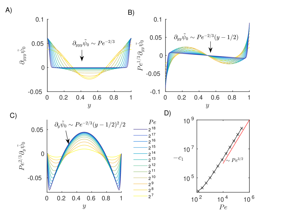
Figure 8: Plots of derivatives of the approximate optimal flows $\tilde{\psi}_{0}\equiv\tilde{\psi}_{1}/c_{1}$ along the channel midline ($x=L/2$) scaled by powers of $Pe$ to show convergence in the wall boundary layers near $y=0$ and 1. We have $\partial_{y}^{3}\tilde{\psi}_{0}\sim Pe^{0}$ (A), $\partial_{y}^{2}\tilde{\psi}_{0}\sim Pe^{-1/3}$ (B), and $\partial_{y}\tilde{\psi}_{0}\sim Pe^{-2/3}$ (C). Outside the boundary layers, the three functions scale like $Pe^{-2/3}$ times polynomials of order 0 (A), 1 (B), and 2 (C). Each line corresponds to a value of $Pe$ listed between panels C and D. Panel D shows the scaling of the normalizing constant defined in (28), $c_{1}\sim Pe^{3/2}$.

Therefore, at a given $x$ away from the upstream and downstream boundaries, we approximate (32)–(33) by

PDE Top BCs Bottom BCs

$$-2\partial_{y}^{4}\tilde{\psi}_{0}=f, \tilde{\psi}_{0}=\partial_{y}\tilde{\psi}_{0}=0, \tilde{\psi}_{0}=\partial_{y}\tilde{\psi}_{0}=0$$ (34)

This is the equation for an elastic beam with clamped-clamped boundary conditions, loaded by sharp concentrations of force density ($-f/2$), equal and opposite in the boundary layers at each end. In appendix B we find approximate scalings of $\tilde{\psi}_{0}$ and its derivatives inside and outside the boundary layers by using a minimization principle from elasticity. Here we give a brief explanation without the details. Since $f$ has boundary layers of width $\sim Pe^{-1/3}$ in $y$, we assume such boundary layers for $\tilde{\psi}_{0}$ and its derivatives. In the boundary layer, taking a $y$-derivative of $\tilde{\psi}_{0}$ is roughly equivalent to multiplying by a factor of $Pe^{1/3}$. Since $\partial_{y}^{4}\tilde{\psi}_{0}\sim f\sim Pe^{1/3}$ in the boundary layer, we expect $\partial_{y}^{3}\tilde{\psi}_{0}\sim Pe^{0}$, $\partial_{y}^{2}\tilde{\psi}_{0}\sim Pe^{-1/3}$, $\partial_{y}\tilde{\psi}_{0}\sim Pe^{-2/3}$ there. These behaviors are shown in figure 8A-C. Outside the boundary layer, we can find the scalings by the top and bottom boundary conditions on $\partial_{y}\tilde{\psi}_{0}$ in (34), which imply

$$0=\partial_{y}\tilde{\psi}_{0}|_{y=1}-\partial_{y}\tilde{\psi}_{0}|_{y=0}=\int_{0}^{1}\partial_{yy}\tilde{\psi}_{0}dy=\int_{\mbox{\small BL}}\partial_{yy}\tilde{\psi}_{0}dy+\int_{\mbox{\small outside BL}}\partial_{yy}\tilde{\psi}_{0}dy.$$ (35)

The contribution inside the boundary layer (denoted “BL” in (35)) has magnitude $\sim Pe^{-1/3}$ in a region of width $\sim Pe^{-1/3}$. To cancel this term, the contribution from outside the boundary layer (denoted “outside BL” in (35)) is over a region of width $\sim 1$, so $\partial_{yy}\tilde{\psi}_{0}$ should have magnitude $\sim Pe^{-2/3}$ there. Since this region has width $\sim 1$, it makes sense that the other $y$-derivatives of $\tilde{\psi}_{0}$ should also have magnitude $\sim Pe^{-2/3}$ in the outer region, as shown in figure 8A-C. Since $\partial^{4}_{y}\tilde{\psi}_{0}\sim f\approx 0$ in this region, $\partial_{y}^{3}\tilde{\psi}_{0}$, $\partial_{y}^{2}\tilde{\psi}_{0}$, and $\partial_{y}\tilde{\psi}_{0}$ are polynomials of degree 0, 1 and 2, respectively, also shown in figure 8A-C. In particular, $\partial_{y}\tilde{\psi}_{0}$ is a parabola in this region, and with an appropriate prefactor $c_{1}$, $\tilde{\psi}_{1}=c_{1}\partial_{y}\tilde{\psi}_{0}$ can cancel the parabolic flow of $\psi_{Pois}$ outside the boundary layers, so the total approximate optimal flow $\partial_{y}\psi_{1}=\psi_{Pois}+c_{1}\partial_{y}\tilde{\psi}_{0}$ is uniform in this region, with zero enstrophy expended.

Having discussed the scalings of $\tilde{\psi}_{0}$ and its $y$-derivatives, we can compute $c_{1}$ from (28) written in terms of $\tilde{\psi}_{0}$, keeping only $y$-derivatives

$$c_{1}\approx\pm 2\sqrt{Pe^{2}-12L\psi_{top}^{2}}\Bigg{/}\sqrt{\int_{0}^{1}\int_{0}^{L}\left(\partial_{y}^{2}\tilde{\psi}_{0}\right)^{2}dxdy}.$$ (36)

In the denominator, the integral has a contribution $\sim Pe^{-1}$ from the boundary layer and $\sim Pe^{-4/3}$ from outside, so it is $\sim Pe^{-1}$. To determine the scaling of $c_{1}$ for the approximate optimal flow, we need to know $\psi_{top}$ for this flow, defined as $\psi_{top,opt}$. We know $\psi_{top,opt}$ is bounded by $\bar{\psi}_{top}$, and so the numerator of (36) is $O(Pe)$ (unless $\psi_{top,opt}\to\bar{\psi}_{top}$ as $Pe\to\infty$, which does not agree with the numerical solutions). Therefore we have $c_{1}\sim Pe^{3/2}$, shown in figure 8D. This constant converts the scalings for $\tilde{\psi}_{0}$ into those for the approximate optimal flow component $\tilde{\psi}_{1}$. For example, $\partial_{y}\tilde{\psi}_{1}=c_{1}\partial_{y}\tilde{\psi}_{0}\sim Pe^{3/2}Pe^{-2/3}=Pe^{5/6}$. The total approximate optimal flow is $\psi_{1}=\psi_{Pois}+\tilde{\psi}_{1}$, which requires knowing the constant $\psi_{top}$ where the optimal heat transfer occurs. We use the intuition from figure 4 that the optimal $\psi_{top}$ is that for which the core flow is a uniform flow with zero enstrophy expended. By figure 8C, $\partial_{y}\tilde{\psi}_{1}$ has a backward parabolic flow $\sim Pe^{5/6}$ outside the boundary layers, so $\psi_{top}\sim Pe^{5/6}$ gives a parabolic flow $\partial_{y}\psi_{Pois}$ which cancels this core flow up to a constant, giving a uniform core flow.

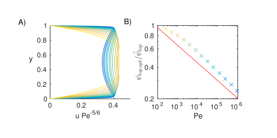
Figure 9: Approximate optimal flows (A) at the $x$ midpoint of the channel for various $Pe=2^{8}$ – $2^{20}$, rescaled by $Pe^{5/6}$. The colors correspond to $Pe$ values marked by crosses in panel B, which also show how the optimal flow rate $\psi_{top,opt}$ decreases relative to that of the starting Poiseuille flow solution, $\bar{\psi}_{top}$. The red line gives the scaling $Pe^{-1/6}$. The channel length is $L=4$.

In figure 9A we plot the approximate optimal flows $u=\partial_{y}\psi_{1}$ over $Pe=2^{8}$ – $2^{20}$ and find a good collapse when divided by $Pe^{5/6}$. The corresponding values of $\psi_{top}/\bar{\psi}_{top}$, denoted $\psi_{top,opt}/\bar{\psi}_{top}$ are plotted in panel B. The red line shows the expected scaling $Pe^{-1/6}$. In fact $\psi_{top,opt}/\bar{\psi}_{top}$ decreases slightly faster. This is reflected in panel A by the fact that the rescaled profiles show a slight decrease with increasing $Pe$. Instead of uniform flow in the core, there is a moderately concave parabolic flow there.

To compute the heat transferred by these flows we need to integrate $\partial_{y}T_{1}$ over the walls, where $T_{1}$ solves (27).

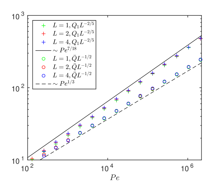
Figure 10: Comparison of the heat transferred by the approximate optimal flows ($Q_{1}$, plusses) with that transferred by the Poiseuille flow at the same value of $Pe$ ($\bar{Q}$, circles), at three channel lengths ($L=1,2$, and 4) at $Pe$ ranging from $2^{7}$ – $2^{21}$. The values are scaled by factors of $L$ as described in the text.

As mentioned earlier, the similarity solution for the temperature field in a Poiseuille flow has heat transfer given by shah2014laminar :

$$\bar{Q}\sim\int_{0}^{L}1.23\left(\frac{2Pe}{x\sqrt{3L}}\right)^{1/3}dx=1.85(4/3)^{1/6}Pe^{1/3}L^{1/2}$$ (37)

The quantity in parentheses in (37) is proportional to the similarity variable $\eta$ raised to the -1/3 power, and is $x$ scaled by the velocity gradient at the wall (i.e. the vorticity) for Poiseuille flow, $\sim Pe/\sqrt{L}$. For the approximate optimal flow, the wall vorticity is proportional to $Pe^{7/6}$. To find the scalings we substitute $Pe^{7/6}$ for $Pe/\sqrt{L}$ in (37), and drop the constants and $L$ dependence (which are altered for the approximate optimal flows). We obtain $Q_{1}\sim Pe^{7/18}$. The discussion of the $L$ dependence is deferred to section VIII. In figure 10 we compare $Q_{1}$ with $\bar{Q}$, the heat transferred by Poiseuille flow, at $Pe$ = $2^{7}$ – $2^{21}$ and three channel lengths ($L=1,2,$ and 4). The data approximately collapse when scaled by $L^{1/2}$ for Poiseuille flow (already discussed) and $L^{2/5}$ for the approximate optimal flows (discussed later, in section VIII). The improvement over Poiseuille flow reaches a factor of 2 near $Pe=10^{6}$ for $L=1$.

VII Fully coupled system

The method of successive approximations in the last section has shown how the initial temperature boundary layer $\sim Pe^{-1/3}$ produces the approximate optimal flow boundary layer, and how that induces a sharper temperature boundary layer $\sim Pe^{-7/18}$ at the next iteration. With this temperature boundary layer, the optimal flow is then modified through the source term in (14) at the next iteration. Proceeding in this way, one would hope to determine the flow and temperature boundary layers that simultaneously solve the fully coupled problem (12)–(16). Computationally it is difficult to achieve convergence with Newton’s method for $Pe\gtrsim 10^{5}-10^{6}$, so we proceed with a unidirectional flow approximation. We might expect the optimal unidirectional flow to be better than the optimal 2D flow field solution in (12)–(16) because that flow is constrained to be Poiseuille flow at the upstream and downstream boundaries, while the optimal unidirectional flow can take on a wider range of values at those locations. The optimal 2D flow field is nearly unidirectional in the middle of the channel, so assuming a unidirectional flow may not sacrifice much.

Let us approximate the optimal flow velocity as unidirectional, $u(y)\mathbf{\hat{e}}_{x}$, with a boundary layer of thickness $\sim Pe^{-\alpha}$. The flow $u(y)$ rises from 0 to a value $\sim Pe^{\beta}$ outside the boundary layer, where the flow is assumed uniform, so the vorticity is zero there. In the boundary layer, the vorticity $\omega=\partial_{y}u\sim Pe^{\beta+\alpha}$.

One equation relating $\alpha$ and $\beta$ is that the total enstrophy is $Pe^{2}$:

$$Pe^{2}=L\int_{0}^{1}\omega^{2}dy\sim Pe^{2\beta+\alpha}\rightarrow 2\beta+\alpha=2.$$ (38)

The thinner the boundary layer (larger $\alpha$), the smaller the velocity inside and outside the boundary layer (smaller $\beta$). Another equation comes from the condition that the temperature boundary layer thickness should have the same scaling as the flow boundary layer thickness. This is essentially what is expressed by equation (14), where the temperature boundary layer appears in $\nabla^{\perp}T\cdot\nabla m$ and creates a flow boundary layer in $\psi$. The relationship between the boundary layers is also shown in figures 7 and 8. The condition is optimal physically because it gives the fastest possible flow in the temperature boundary layer, so it convects the most heat out of the channel. If instead the flow boundary layer were smaller than the temperature boundary layer (i.e. increased $\alpha$), by (38) the flow speed magnitude would be reduced everywhere (decreased $\beta$) including the temperature boundary layer, so less heat would be convected out of the channel. If on the other hand the flow boundary layer were larger than the temperature boundary layer, then enstrophy is being spent to create a faster core flow at the expense of enstrophy in the boundary layer. Since the temperature is uniformly zero in the core, there is no advantage to having a faster flow there, while the slower boundary layer flow convects less heat. The similarity solution tells us how the temperature boundary layer is related to the flow boundary layer. In the flow boundary layer, $u\sim Pe^{\beta+\alpha}y$. Assuming this profile holds throughout the temperature boundary layer, we can apply the similarity solution for the temperature field in a linear velocity profile leveque1928laws , giving the temperature boundary layer thickness $\sim|$wall vorticity$|^{-1/3}=|\partial_{y}u|^{-1/3}$ $\sim Pe^{-(\beta+\alpha)/3}$. Setting this equal to the flow boundary layer thickness gives

$$Pe^{-(\beta+\alpha)/3}\sim Pe^{-\alpha}\rightarrow\beta=2\alpha.$$ (39)

Combining (38) and (39) yields $\alpha=2/5$ and $\beta=4/5$.

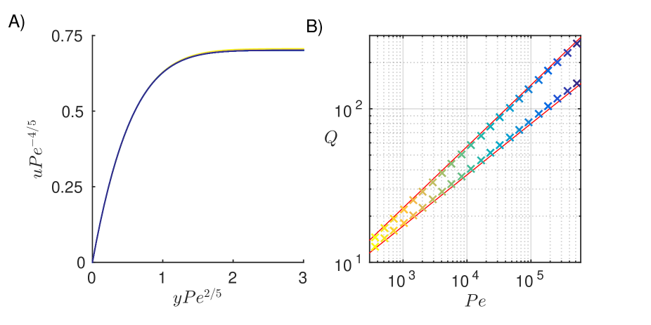
Figure 11: Optimal unidirectional flows $u(y)$ and heat transferred. A) For $Pe$ ranging from $2^{8.5}$ to $2^{19}$ in multiplicative increments of $2^{0.5}$, the optimal unidirectional flow profiles near the lower wall, with $u$ rescaled by $Pe^{4/5}$ and $y$ scaled by $Pe^{-2/5}$. B) The heat transferred by the optimal unidirectional flow (upper set of crosses), with scaling line $Pe^{2/5}$ (upper red line), and the heat transferred by the Poiseuille flow at the same $Pe$ (lower set of crosses), with scaling line $Pe^{1/3}$ (lower red line). Here $L$ = 1 and $\delta=0.1$. The colors for the 22 lines in panel A correspond to the colors of the crosses in panel B at the same $Pe$.

These values can also be derived another way. Instead of assuming flow boundary layer thickness $\sim$ temperature boundary layer thickness, we can allow it to arise naturally in the optimization. We want to maximize $\partial_{y}T$ (actually its integral over $x$), and $T$ falls from 1 to 0 over the temperature boundary layer, so $\partial_{y}T\sim$ (temperature boundary layer thickness)^-1. If the flow boundary layer is much larger than the temperature boundary layer, the temperature evolves in a linear shear flow, and the boundary layer thickness $\sim\omega_{wall}^{-1/3}\sim Pe^{-(\beta+\alpha)/3}\sim Pe^{-(1+\alpha/2)/3}$ using (38) to eliminate $\beta$. If the flow boundary layer is much smaller than the temperature boundary layer, the temperature evolves in an essentially uniform flow, with boundary layer thickness $\sim$ (flow speed)^-1/2. This follows from the similarity solution for the temperature in a uniform flow field haase2015graetz ; graetz1882ueber , the same as the similarity solution to the heat equation in one space and one time variable. We have boundary layer thickness $\sim$ (flow speed)${}^{-1/2}\sim Pe^{-\beta/2}\sim Pe^{-(1-\alpha/2)/2}$ using (38) again to eliminate $\beta$. At $\alpha=2/5$, both expressions give the temperature boundary layer thickness $\sim Pe^{-2/5}$, the same as the flow boundary layer. If the flow boundary layer were smaller, then $\alpha>(1-\alpha/2)/2\rightarrow(1-\alpha/2)/2\leq 2/5$, so the temperature boundary layer would be larger than $Pe^{-2/5}$. If the flow boundary layer were larger, then $\alpha\leq(1+\alpha/2)/3\rightarrow(1+\alpha/2)/3\leq 2/5$, and again the temperature boundary layer would be larger than $Pe^{-2/5}$. The optimum occurs when the temperature boundary layer has the smallest thickness, $\sim Pe^{-2/5}$, which is when the flow and temperature boundary layer thicknesses are equal. In this case, the heat transfer scales as $Pe^{2/5}$, which is slightly greater than that for the first iteration of the method of successive approximations ($Pe^{7/18}$), about 16% greater at $Pe=10^{6}$. This slight difference may explain the close agreement between the exact and approximate heat transfer in figure 5. The improvement of $Pe^{2/5}$ over the $Pe^{1/3}$ scaling for Poiseuille flow is a factor of about 2.5 at $Pe=10^{6}$ with $L=1$.

To test these hypotheses we employ a quasi-Newton (Broyden) method to solve for the optimal $u(y)$ using equations (12)–(16) specialized to the case $\psi(x,y)\equiv\psi(y)$, with no boundary conditions needed for $\psi$ at the $x$-boundaries. $T$ and $m$ are still functions of $x$ and $y$ with the same boundary conditions. Unlike Newton’s method, Broyden’s method uses a dense approximation to the Jacobian matrix, but it is manageable since $\psi(y)$ is discretized on a 1D grid in $y$. An important savings comes from the fact that $\partial_{y}^{3}\psi(y)$ is constant outside the boundary layer, so we only need to explicitly compute $\partial_{y}\psi(y)$ in a region slightly larger than the boundary layer, and can represent $\partial_{y}\psi(y)$ outside by a quadratic polynomial that matches the solution slightly outside the boundary layer. Only 90 unknowns are used in this version of Broyden’s method, though ill-conditioning is still an issue as the boundary layer shrinks.

In figure 11 we plot the results of the unidirectional flow optimization. Panel A shows the flow profiles near the boundary layer for $Pe$ ranging from $2^{8.5}$ to $2^{19}$ in multiplicative increments of $2^{0.5}$, with $u$ scaled by $Pe^{4/5}$ and $y$ scaled by $Pe^{-2/5}$, showing the expected behaviors. Panel B shows the heat transferred by these flows (upper set of crosses), with scaling $Q\sim Pe^{2/5}$, compared to the Poiseuille flow at the same $Pe$ (lower set of crosses), with scaling $Q\sim Pe^{1/3}$.

VIII Effect of varying $L$

We now discuss the dependence of solutions on the other main parameter, $L$, the channel length/height. With fixed enstrophy, as $L$ increases, the enstrophy spreads out, and therefore the flow is weaker, which leads to a thicker temperature boundary layer. The boundary layer is also thicker on average in the channel because it spreads as $x$ increases (for $T$) or $L-x$ increases (for $m$). Therefore, we expect the optimal solutions to have a thicker boundary layer and slower flows at larger $L$, opposite to the effects of increasing $Pe$ with fixed $L$.

To determine how the optimal solutions scale with $L$ at fixed $Pe$, we can use two methods. The first is the same as for the $Pe$ scalings: find power law exponents for 1. the boundary layer thickness and 2. the maximum flow speed such that 1. the flow and temperature boundary layers have the same scaling law and 2. total enstrophy scales as $Pe^{2}$, i.e. is $L$-independent. Let us assume the the optimal flow and temperature fields have boundary layer thicknesses $\sim L^{-\alpha}$, and that the optimal flow speed has a maximum value $\sim L^{\beta}$.

With fixed enstrophy (fixed $Pe$),

$$L^{0}\sim L\int_{0}^{1}\omega^{2}dy\sim L^{1}L^{2(\beta+\alpha)}L^{-\alpha}\rightarrow 1+\alpha+2\beta=0.$$ (40)

The temperature boundary layer thickness, which has the same thickness as the flow boundary layer via (14)), scales as (wall vorticity)${}^{-1/3}\sim L^{(-\alpha-\beta)/3}$, and spreads like $x^{1/3}\sim L^{1/3}$ in a channel of length $L$. Matching this to the flow boundary layer thickness,

$$L^{(-\alpha-\beta)/3}L^{1/3}\sim L^{-\alpha}\rightarrow-\alpha/3-\beta/3+1/3=-\alpha.$$ (41)

Solving (40) and (41) we have $\alpha=-3/5$ and $\beta=-1/5$.

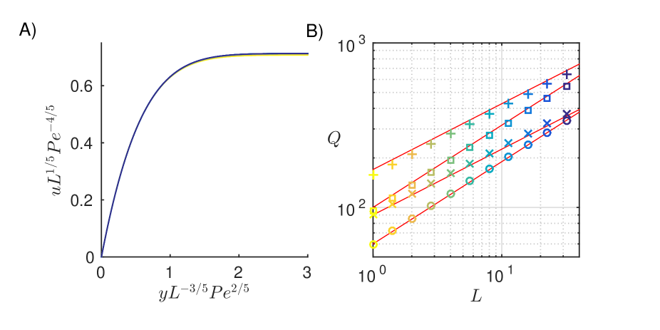
Figure 12: Scalings of optimal unidirectional flows with $L$. A, Optimal unidirectional flows with fixed enstrophy at $L$ varying from 1 to 32 in factors of $\sqrt{2}$, at $Pe=2^{15}$ and $2^{17}$. B, Corresponding heat transferred $Q$ versus $L$ at $Pe=2^{15}$ (crosses for optimal flows and circles for Poiseuille flows) and $Pe=2^{17}$ (plusses for optimal flows and squares for Poiseuille flows). The red lines near the optimal-flow data give the scaling $L^{2/5}$ while those near the Poiseuille-flow data give the scaling $L^{1/2}$.

Figure 12A shows the numerical solutions collapsed with the appropriate scalings in $L$ and $Pe$ applied simultaneously. We vary $L$ from 1 to 32 in factors of $\sqrt{2}$, and at two different $Pe$, $2^{15}$ and $2^{17}$, yielding 22 curves which are collapsed in panel A. Larger $L$ is challenging for computations because of the large grid needed to cover the domain at a given resolution. The scaling for $Q$ is given by

$$Q=2\int_{0}^{L}\partial_{y}T|_{y=0}dx\sim\int_{0}^{L}\left(\frac{L^{(\alpha+\beta)/3}}{x}\right)^{1/3}dx\sim L^{2/5}.$$ (42)

In (42) we have used the fact that the temperature boundary layer thickness scales as (wall vorticity)${}^{-1/3}\sim L^{(\alpha+\beta)/3}$, and grows as $x^{1/3}$ in the linear-flow similarity solution. In (42), the heat flux is proportional to the inverse of the temperature boundary layer thickness, so we are integrating the reciprocal of these terms. The optimal heat flux scaling $Q\sim L^{2/5}$ is shown by the plusses and crosses in figure 12B, and compared with the $L^{1/2}$ scalings for the starting uniform flows at the same $Pe$ and $L$ (squares and circles). The two diverge as $L$ becomes smaller, where the boundary layers are thinner and there is a greater advantage to concentrating the flow in the boundary layer.

There is a second way to determine the optimal scalings with $L$. It is to recognize that the boundary layers have no dependence on the channel height, $H$ (dimensional) or 1 (dimensionless). Therefore, in the boundary layer regime, there is only one relevant length scale in the problem, $L_{0}$ (dimensional channel length). By using $L_{0}$ instead of $H$ as the length scale, we can eliminate one dimensionless parameter, $L$ say. So long as the boundary layer is much smaller than $H$, the solutions do not depend on $L=L_{0}/H$, only the energy/enstrophy budget, which needs to be redefined as $\tilde{Pe}$ instead of $Pe$ when $L_{0}$ is the length scale. All the information is contained in the problem as a function of $\tilde{Pe}$, so it should yield the scalings with respect to $L$ and $Pe$ separately. Indeed, we can obtain the scalings using this approach, as shown in Appendix C.

IX Physical considerations

We have given results in terms of $Pe$, similarly to hassanzadeh2014wall ; souza2015transport ; goluskin2016bounds ; tobasco2016optimal ; alben_2017 , because this measures the energy of the flow, the key constraint in our problem. To estimate the physical scales of these flows, we now list the Reynolds numbers corresponding to the flows we have computed for the most common convecting fluid, air.

For the case of fixed enstrophy = $Pe^{2}$, the dimensionless Poiseuille flow $u(y)=6Pe(y-y^{2})/\sqrt{12L}$ has $y$-averaged flow speed $\langle u\rangle=Pe/\sqrt{12L}$. The corresponding dimensional flow speed is $\langle u\rangle\kappa/H$. Using this flow speed and the channel height $H$ as a typical length, we define the Reynolds number as

$$Re\equiv\frac{Pe}{\sqrt{12L}}\frac{\kappa}{H}\frac{H}{\nu}=\frac{Pe}{\sqrt{12L}}\frac{1}{Pr}.$$ (43)

where $Pr=\nu/\kappa$ is the Prandtl number, about 0.8 for air at 300K. Therefore $Pe=10^{5}$ corresponds to $Re=10^{4}-3\times 10^{4}$ for Poiseuille flow with $L$ ranging from 1 to 8. The optimal flows shown in figure 12A grow more slowly with increasing $Pe$ and decrease more slowly with increasing $L$: $\langle u\rangle\approx 0.7L^{-1/5}Pe^{4/5}$. At $Pe=10^{5}$, $Re=4000-7000$ for $L=1-8$. At $Pe=10^{5}$ we have significant improvement in heat transfer, about a factor of $1.6$ over Poiseuille flow at $L=1$. The corresponding $Re$ are near the critical values for the transition to turbulence in plane Poiseuille flow, $Re$ = 5772 for the linear instability, about 2900 for finite-amplitude disturbances, and about 1000 in experiments due to 3D effects schmid2012stability . These values will undoubtedly change for the optimal flow profiles. Since the instability is convective, the transition may occur sufficiently slowly that the flow remains laminar in the moderate-length channels considered here schmid2012stability ; shah2014laminar and in heat sink geometries hamburgen1986optimal .

A steady unidirectional flow $u(y)$ is produced by a pressure gradient $\partial_{x}p=\nu\partial_{yy}u$. For the optimal flows with fixed enstrophy in figure 12A, this function has a maximum at the wall and decreases to zero outside the boundary layer. One could achieve an approximation to this pressure gradient with fans $\sim Pe^{-2/5}$ in size placed adjacent to the wall at the upstream and downstream boundaries, to produce the boundary layers of the appropriate sizes.

X Conclusion

In this paper we have computed sequences of optimal flows for heat transfer in a channel. They are only locally optimal, and proceed from a particular initial solution: Poiseuille flow. However, they give a lower bound on the improvement that can be obtained over this fundamental flow.

Poiseuille flow is perhaps the most common laminar flow in a duct or channel, the result of a uniform pressure gradient. The sequence of steady 2D flows we have computed starting from Poiseuille flow are optimal under the constraint of a fixed rate of viscous dissipation, $Pe^{2}$, equal to the power needed to pump the fluid through the channel. They are well-approximated by the optimal unidirectional flows we computed, which have a boundary layer of thickness $\sim Pe^{-2/5}$ where the flow rises sharply to a maximum speed $\sim Pe^{4/5}$ where the boundary layer meets the core flow. In the core, the flow is uniform, no energy is dissipated, and the fluid temperature is zero, so it does not carry any heat out of the channel. These results can be obtained by the simple condition that the flow and temperature field should have boundary layer thicknesses of the same order at the optimum.

Using a decoupled approximation, we have shown mathematically how the temperature boundary layer produces an increased flow near the boundaries in the optimal solutions, by depleting the parabolic flow from the initial Poiseuille flow in the core of the channel.

A good approximation to the optimal flows can be produced simply, by changing the uniform pressure gradient of Poiseuille flow to one that is localized in the boundary layer, with unidirectional forcing (e.g. fans) localized in the boundary layer. In an appendix we show how to compute the 2D forcing field that corresponds to any given flow field as the solution to coupled Poisson problems.

We have also shown that in a channel of aspect ratio (length/height) $L$, the boundary layer thickness scales as $L^{3/5}$ and the outer flow speed scales as $L^{-1/5}$ for the optimal unidirectional flow. The results are obtained by again matching the temperature and flow boundary layer thicknesses for the optimal solution, or by using dimensional analysis (in an appendix), noting that the boundary layer solutions do not depend on the channel height.

We have found a 60% improvement in heat transfer over Poiseuille flow at the same pumping power, at Reynolds numbers where the Poiseuille flow becomes unstable, using air as the convecting fluid. This value is for aspect ratio $L=1$; the improvement increases with shorter channels. In future work these approaches can be extended to unsteady 3D flows, which show promise for further heat transfer improvements rips2017efficient .

Appendix A Solving for $\mathbf{f}$ and $p$

We can compute $\mathbf{f}$ and $p$ from (5) given $\mathbf{u}$. We use the Helmholtz-Hodge decomposition to write

$$\mathbf{f}=-\nabla\phi+\nabla^{\perp}q.$$ (44)

The irrotational part $-\nabla\phi$ can be absorbed into the pressure gradient in (5). We are left with the incompressible part $\mathbf{f}=\nabla^{\perp}q$. Inserting into (5) we have, for steady flows

$$\rho\mathbf{u}\cdot\nabla\mathbf{u}=-\nabla p+\mu\Delta\mathbf{u}+\nabla^{\perp}q.$$ (45)

Taking the divergence of (45) and using $\nabla\cdot\mathbf{u}=0$ results in a Poisson problem for $p$:

$$-\Delta p=\rho\nabla\cdot\left(\mathbf{u}\cdot\nabla\mathbf{u}\right),$$ (46)

and taking $\nabla^{\perp}\cdot$ (45) gives a Poisson problem for $q$:

$$-\Delta q=-\mu\Delta\omega+\rho\mathbf{u}\cdot\nabla\omega.$$ (47)

where $\omega=\nabla^{\perp}\cdot\mathbf{u}$ is the vorticity. When the velocity field is known, so are the right hand sides of (46) and (47). Coupled Neumann and Dirichlet boundary conditions for (46) and (47) are obtained by taking the normal and tangential components of (45) at the boundaries:

$$\hat{\mathbf{n}}\cdot\left(\rho\mathbf{u}\cdot\nabla\mathbf{u}-\mu\Delta\mathbf{u}\right) =-\partial_{n}p+\partial_{s}q.$$ (48)

$$\hat{\mathbf{s}}\cdot\left(\rho\mathbf{u}\cdot\nabla\mathbf{u}-\mu\Delta\mathbf{u}\right) =-\partial_{s}p-\partial_{n}q.$$ (49)

where $s$ and $n$ denote coordinates tangential and normal to the boundary. This is analogous to the derivation of Neumann pressure boundary conditions in gresho1987pressure .

Appendix B Estimating the boundary layer scalings by minimizing the elastic energy of a beam

The beam equation arises from the principle of minimum total potential energy in elasticity landau1986te ; renton2002elastic . At a given $x$ away from the $x$ boundaries, our flow is analogous to a beam with deflection $\tilde{\psi}_{0}(y)$ with bending modulus 2 and force density $-f$, which minimizes

$$U_{elastic}=\int_{0}^{1}(\partial_{y}^{2}\tilde{\psi}_{0})^{2}+f\tilde{\psi}_{0}\,dy$$ (50)

The first term in (50) is the internal elastic energy due to beam curvature, and also our enstrophy constraint neglecting $x$-dependence of $\tilde{\psi}_{0}$. The second term in (50) is minus the work done by $f$ (and corresponds to the advection-diffusion equation constraint for our flow). Using the clamp boundary conditions in (34),

$$U_{elastic}=\int_{0}^{1}\left[(\partial_{y}^{2}\tilde{\psi}_{0})^{2}+f\int_{0}^{y}\int_{0}^{y^{\prime}}\partial_{y^{\prime\prime}}^{2}\tilde{\psi}_{0}dy^{\prime\prime}dy^{\prime}\right]\,dy.$$ (51)

We assume $\partial_{y}^{2}\tilde{\psi}_{0}\sim Pe^{\alpha}$ in the boundary layer and find $\alpha$ by assuming that both terms in $U_{elastic}$ are of the same order when $U_{elastic}$ is minimized. Using $f\sim Pe^{1/3}$ and that each integration over the boundary layer gives a factor of $Pe^{-1/3}$, the two terms in (51) become

$$Pe^{2\alpha}Pe^{-1/3}\sim Pe^{1/3}Pe^{\alpha}Pe^{-1}$$ (52)

which implies $\alpha=-1/3$. In figure 8a–c we plot $\partial_{y}^{3}\tilde{\psi}_{0}$, $\partial_{y}^{2}\tilde{\psi}_{0}$, and $\partial_{y}\tilde{\psi}_{0}$ respectively along the channel midline ($x=L/2$) for $L=4$ and various $Pe$ (listed between panels c and d). We find that each function has a boundary layer behavior consistent with what we’ve described. In panel b, we find $\partial_{y}^{2}\tilde{\psi}_{0}\sim Pe^{-1/3}$ in the boundary layer. Differentiating with respect to $y\sim Pe^{-1/3}$ in the boundary layer yields $\partial_{y}^{3}\tilde{\psi}_{0}\sim Pe^{0}$ (panel a), and integrating yields $\partial_{y}\tilde{\psi}_{0}\sim Pe^{-2/3}$ (panel c). These panels also show that outside the boundary layers, all three functions scale like $Pe^{-2/3}$ times polynomials of order 0 ($\partial_{y}^{3}\tilde{\psi}_{0}$, panel a), 1 ($\partial_{y}^{2}\tilde{\psi}_{0}$, panel b), and 2 ($\partial_{y}\tilde{\psi}_{0}$, panel c). The polynomial orders are consistent with $\partial_{y}^{4}\tilde{\psi}_{0}\sim f\approx 0$ outside the boundary layers.

To understand the scalings outside the boundary layers we write an approximation for $\partial_{y}^{2}\tilde{\psi}_{0}$, valid inside and outside the boundary layers, as $a_{1}(\eta)Pe^{-1/3}+a_{2}(y)Pe^{\beta}$. Plugging this expression into $U$, we have an increased energy outside the boundary layer with a decreased energy inside the boundary layer, if the sign of $a_{2}(0)$ is opposite that of $a_{1}(\eta)$ as $\eta\to\infty$. Both energies are of the same order if $\beta=-2/3$, and a net energy decrease occurs for an appropriate choice of $a_{2}(y)$.

Appendix C $L$ scalings using alternative nondimensionalization

We define a new system of dimensionless quantities with $L_{0}$ as the characteristic length instead of $H$, and denote them with tildes. First, we relate $\tilde{Pe}$ to $Pe$. With fixed enstrophy,

$$Pe^{2}=\frac{\dot{E}H^{2}}{W\mu\kappa^{2}}=\frac{\dot{E}L_{0}^{2}}{W\mu\kappa^{2}}\frac{H^{2}}{L_{0}^{2}}=\tilde{Pe}^{2}L^{-2}.$$ (53)

The scalings for the optimal flow boundary layer thickness $\tilde{q}$, maximum flow speed $\tilde{U}$, and heat transferred $\tilde{Q}$ with respect to $\tilde{Pe}$ are the same as the scalings of the corresponding quantities ($q,U,Q$) with respect to $Pe$ with any fixed value of $L$ (that yields boundary-layer solutions):

$$\frac{q}{L} =\frac{q_{d}}{H}\frac{H}{L_{0}}=\frac{q_{d}}{L_{0}}=\tilde{q}\sim\tilde{Pe}^{-2/5}=Pe^{-2/5}L^{-2/5}\rightarrow q\sim Pe^{-2/5}L^{3/5}$$ (54)

$$UL =\frac{U_{d}H}{\kappa}\frac{L_{0}}{H}=\frac{U_{d}L_{0}}{\kappa}=\tilde{U}\sim\tilde{Pe}^{4/5}=Pe^{4/5}L^{4/5}\rightarrow U\sim Pe^{4/5}L^{-1/5}$$ (55)

$$Q =\tilde{Q}\sim\tilde{Pe}^{2/5}=Pe^{2/5}L^{2/5}.$$ (56)

We have denoted the dimensional quantities by subscript $d$, which allows us to translate between the dimensionless sets ($q,U,Q,Pe$) and ($\tilde{q},\tilde{U},\tilde{Q},\tilde{Pe}$).

These are the same scalings as in Section VIII.

References

- [1] Frank Kreith, Raj M Manglik, and Mark S Bohn. Principles of heat transfer. Cengage learning, 2012.
- [2] David Reay, Colin Ramshaw, and Adam Harvey. Process Intensification: Engineering for efficiency, sustainability and flexibility. Butterworth-Heinemann, 2013.
- [3] Jun Dai, Michael M Ohadi, Diganta Das, and Michael G Pecht. Optimum cooling of data centers. Springer, 2014.
- [4] Yogendra Joshi and Pramod Kumar. Energy efficient thermal management of data centers. Springer Science & Business Media, 2012.
- [5] Michael K Patterson, Shankar Krishnan, and John M Walters. On energy efficiency of liquid cooled hpc datacenters. In Thermal and Thermomechanical Phenomena in Electronic Systems (ITherm), 2016 15th IEEE Intersociety Conference on, pages 685–693. IEEE, 2016.
- [6] Guy R Wagner, Joseph R Schaadt, Justin Dixon, Gary Chan, William Maltz, Kamal Mostafavi, and David Copeland. Test results from the comparison of three liquid cooling methods for high-power processors. In Thermal and Thermomechanical Phenomena in Electronic Systems (ITherm), 2016 15th IEEE Intersociety Conference on, pages 619–624. IEEE, 2016.
- [7] Wataru Nakayama. Thermal management of electronic equipment: a review of technology and research topics. Applied Mechanics Reviews, 39(12):1847–1868, 1986.
- [8] M Zerby and M Kuszewski. Final report on next generation thermal management (NGTM) for power electronics. Technical report, NSWCCD Technical Report TR-82-2002012, 2002.
- [9] Ryan J McGlen, Roshan Jachuck, and Song Lin. Integrated thermal management techniques for high power electronic devices. Applied thermal engineering, 24(8):1143–1156, 2004.
- [10] Mark F Ahlers. Aircraft Thermal Management. Encyclopedia of Aerospace Engineering, 2011.
- [11] JC Hart, JS Park, and CK Lei. Heat transfer enhancement in channels with turbulence promoters. Journal of Engineering for Gas Turbines and Power, 107:628–635, 1985.
- [12] Dennis Leroy Gee and RL Webb. Forced convection heat transfer in helically rib-roughened tubes. International Journal of Heat and Mass Transfer, 23(8):1127–1136, 1980.
- [13] JP Tsia and JJ Hwang. Measurements of heat transfer and fluid flow in a rectangular duct with alternate attached–detached rib-arrays. International journal of heat and mass transfer, 42(11):2071–2083, 1999.
- [14] Pongjet Promvonge, Teerapat Chompookham, Sutapat Kwankaomeng, and Chinaruk Thianpong. Enhanced heat transfer in a triangular ribbed channel with longitudinal vortex generators. Energy Conversion and Management, 51(6):1242–1249, 2010.
- [15] Kourosh Shoele and Rajat Mittal. Computational study of flow-induced vibration of a reed in a channel and effect on convective heat transfer. Physics of Fluids, 26(12):127103, 2014.
- [16] Martin Fiebig, Peter Kallweit, Nimai Mitra, and Stefan Tiggelbeck. Heat transfer enhancement and drag by longitudinal vortex generators in channel flow. Experimental Thermal and Fluid Science, 4(1):103–114, 1991.
- [17] Atul Sharma and V Eswaran. Heat and fluid flow across a square cylinder in the two-dimensional laminar flow regime. Numerical Heat Transfer, Part A: Applications, 45(3):247–269, 2004.
- [18] Tolga Açıkalın, Suresh V Garimella, Arvind Raman, and James Petroski. Characterization and optimization of the thermal performance of miniature piezoelectric fans. International Journal of Heat and Fluid Flow, 28(4):806–820, 2007.
- [19] Donavon R Gerty. Fluidic driven cooling of electronic hardware. Part I: Channel integrated vibrating reed. Part II: Active heat sink. PhD thesis, 2008.
- [20] Pable Hidalgo, Florian Herrault, Ari Glezer, Mark Allen, Scott Kaslusky, and Brian St Rock. Heat transfer enhancement in high-power heat sinks using active reed technology. In Thermal Investigations of ICs and Systems (THERMINIC), 2010 16th International Workshop on, pages 1–6. IEEE, 2010.
- [21] Sourabh Jha, Pablo Hidalgo, and Ari Glezer. Small-scale vortical motions induced by aeroelastically fluttering reed for enhanced heat transfer in a rectangular channel. Bulletin of the American Physical Society, 60, 2015.
- [22] Silas Alben. Flag flutter in inviscid channel flow. Physics of Fluids, 27(3):033603, 2015.
- [23] Xiaolin Wang and Silas Alben. The dynamics of vortex streets in channels. Physics of Fluids, 27(7):073603, 2015.
- [24] Ramesh K Shah and Alexander Louis London. Laminar flow forced convection in ducts: a source book for compact heat exchanger analytical data. Academic press, 2014.
- [25] Warren M Rohsenow, James P Hartnett, Young I Cho, et al. Handbook of heat transfer. McGraw-Hill New York, 1998.
- [26] M.A. Lévêque. Les lois de la transmission de chaleur par convection. Les Annales des Mines: Memoires, 12(13):201–299, 1928.
- [27] von L Graetz. Ueber die wärmeleitungsfähigkeit von flüssigkeiten. Annalen der Physik, 254(1):79–94, 1882.
- [28] Frédéric De Gournay, Jérôme Fehrenbach, and Franck Plouraboué. Shape optimization for the generalized graetz problem. Structural and Multidisciplinary Optimization, 49(6):993–1008, 2014.
- [29] A Sander Haase, S Jonathan Chapman, Peichun Amy Tsai, Detlef Lohse, and Rob GH Lammertink. The graetz–nusselt problem extended to continuum flows with finite slip. Journal of fluid mechanics, 764:R3, 2015.
- [30] Andre N Souza and Charles R Doering. Maximal transport in the Lorenz equations. Physics Letters A, 379(6):518–523, 2015.
- [31] Andre N Souza and Charles R Doering. Transport bounds for a truncated model of Rayleigh–Bénard convection. Physica D: Nonlinear Phenomena, 308:26–33, 2015.
- [32] Andre N Souza. An Optimal Control Approach to Bounding Transport Properties of Thermal Convection. PhD thesis, 2016.
- [33] W-L Chien, H Rising, and JM Ottino. Laminar mixing and chaotic mixing in several cavity flows. Journal of Fluid Mechanics, 170:355–377, 1986.
- [34] CP Caulfield and RR Kerswell. Maximal mixing rate in turbulent stably stratified Couette flow. Physics of Fluids, 13(4):894–900, 2001.
- [35] W Tang, CP Caulfield, and RR Kerswell. A prediction for the optimal stratification for turbulent mixing. Journal of Fluid Mechanics, 634:487–497, 2009.
- [36] Becca Thomases, Michael Shelley, and Jean-Luc Thiffeault. A Stokesian viscoelastic flow: Transition to oscillations and mixing. Physica D: Nonlinear Phenomena, 240(20):1602–1614, 2011.
- [37] DPG Foures, CP Caulfield, and Peter J Schmid. Optimal mixing in two-dimensional plane Poiseuille flow at finite Péclet number. Journal of Fluid Mechanics, 748:241–277, 2014.
- [38] R Camassa, Z Lin, RM McLaughlin, K Mertens, C Tzou, J Walsh, and B White. Optimal mixing of buoyant jets and plumes in stratified fluids: theory and experiments. Journal of Fluid Mechanics, 790:71–103, 2016.
- [39] Fabian Waleffe, Anakewit Boonkasame, and Leslie M Smith. Heat transport by coherent Rayleigh-Bénard convection. Physics of Fluids, 27(5):051702, 2015.
- [40] David Sondak, Leslie M Smith, and Fabian Waleffe. Optimal heat transport solutions for Rayleigh–Bénard convection. Journal of Fluid Mechanics, 784:565–595, 2015.
- [41] RR Kerswell, CCT Pringle, and AP Willis. An optimization approach for analysing nonlinear stability with transition to turbulence in fluids as an exemplar. Reports on Progress in Physics, 77(8):085901, 2014.
- [42] AK Kaminski, CP Caulfield, and JR Taylor. Transient growth in strongly stratified shear layers. Journal of Fluid Mechanics, 758:R4, 2014.
- [43] Marina Pausch and Bruno Eckhardt. Direct and noisy transitions in a model shear flow. Theoretical and Applied Mechanics Letters, 5(3):111–116, 2015.
- [44] Pedram Hassanzadeh, Gregory P Chini, and Charles R Doering. Wall to wall optimal transport. Journal of Fluid Mechanics, 751:627–662, 2014.
- [45] David Goluskin and Charles R Doering. Bounds for convection between rough boundaries. Journal of Fluid Mechanics, 804:370–386, 2016.
- [46] Ian Tobasco and Charles R Doering. Optimal wall-to-wall transport by incompressible flows. arXiv preprint arXiv:1612.05199, 2016.
- [47] S. Alben. Optimal convection cooling flows in general 2d geometries. Journal of Fluid Mechanics, 814:484–509, 2017.
- [48] MI Campbell, CH Amon, and J Cagan. Optimal three-dimensional placement of heat generating electronic components. Journal of Electronic Packaging, 119(2):106–113, 1997.
- [49] AK Da Silva, S Lorente, and A Bejan. Optimal distribution of discrete heat sources on a wall with natural convection. International Journal of Heat and Mass Transfer, 47(2):203–214, 2004.
- [50] Deepak Gopinath, Yogendra Joshi, and Shapour Azarm. An integrated methodology for multiobjective optimal component placement and heat sink sizing. Components and Packaging Technologies, IEEE Transactions on, 28(4):869–876, 2005.
- [51] George E Karniadakis, Bora B Mikic, and Anthony T Patera. Minimum-dissipation transport enhancement by flow destabilization: Reynolds’ analogy revisited. Journal of Fluid Mechanics, 192:365–391, 1988.
- [52] Bijan Mohammadi, Olivier Pironneau, B Mohammadi, and Oliver Pironneau. Applied shape optimization for fluids, volume 28. Oxford University Press Oxford, 2001.
- [53] VD Zimparov, AK Da Silva, and A Bejan. Thermodynamic optimization of tree-shaped flow geometries. International Journal of Heat and Mass Transfer, 49(9):1619–1630, 2006.
- [54] Qun Chen, Xin-Gang Liang, and Zeng-Yuan Guo. Entransy theory for the optimization of heat transfer–a review and update. International Journal of Heat and Mass Transfer, 63:65–81, 2013.
- [55] Horace Lamb. Hydrodynamics. Cambridge University Press, 1932.
- [56] B. E. Griffith, R. D. Hornung, D. M. McQueen, and C. S. Peskin. An adaptive, formally second order accurate version of the immersed boundary method. J. Comput. Phys., 223:10–49, 2007.
- [57] Aaron Rips, Kourosh Shoele, Ari Glezer, and Rajat Mittal. Efficient electronic cooling via flow-induced vibrations. In Thermal Measurement, Modeling & Management Symposium (SEMI-THERM), 2017 33rd, pages 36–39. IEEE, 2017.
- [58] Franz Durst. Fluid mechanics: an introduction to the theory of fluid flows. Springer Science & Business Media, 2008.
- [59] George C Hsiao and Wolfgang L Wendland. Boundary integral equations. Springer, 2008.
- [60] PM Worsøe-Schmidt. Heat transfer in the thermal entrance region of circular tubes and annular passages with fully developed laminar flow. International Journal of Heat and Mass Transfer, 10(4):541–551, 1967.
- [61] Chia-Chʻiao Lin and Lee A Segel. Mathematics applied to deterministic problems in the natural sciences. SIAM, 1988.
- [62] Sam Howison. Practical applied mathematics: modelling, analysis, approximation. Number 38. Cambridge university press, 2005.
- [63] Peter J Schmid and Dan S Henningson. Stability and transition in shear flows, volume 142. Springer Science & Business Media, 2012.
- [64] William R Hamburgen. Optimal finned heat sinks. Digital Equipment Corporation Western Research Laboratory [WRL], 1986.
- [65] Philip M Gresho and Robert L Sani. On pressure boundary conditions for the incompressible navier-stokes equations. International Journal for Numerical Methods in Fluids, 7(10):1111–1145, 1987.
- [66] ED Landau and EM Lifshitz. Theory of Elasticity. Pergamon Press, Headington Hill Hall, Oxford OX 3 0 BW, UK, 1986., 1986.
- [67] John D Renton. Elastic beams and frames. Elsevier, 2002.