Functional renormalization-group approach to the Pokrovsky-Talapov model via modified massive Thirring fermion model

Abstract

A possibility of the topological Kosterlitz-Thouless (KT) transition in the Pokrovsky-Talapov (PT) model is investigated by using the functional renormalization-group (RG) approach by Wetterich. Our main finding is that the nonzero misfit parameter of the model, which can be related with the linear gradient term (Dzyaloshinsky-Moriya interaction), makes such a transition impossible, what contradicts the previous consideration of this problem by non-perturbative RG methods. To support the conclusion the initial PT model is reformulated in terms of the 2D theory of relativistic fermions using an analogy between the 2D sine-Gordon and the massive Thirring models. In the new formalism the misfit parameter corresponds to an effective gauge field that enables to include it in the RG procedure on an equal footing with the other parameters of the theory. The Wetterich equation is applied to obtain flow equations for the parameters of the new fermionic action. We demonstrate that these equations reproduce the KT type of behavior if the misfit parameter is zero. However, any small nonzero value of the quantity rules out a possibility of the KT transition. To confirm the finding we develop a description of the problem in terms of the 2D Coulomb gas model. Within the approach the breakdown of the KT scenario gains a transparent meaning, the misfit gives rise to an effective in-plane electric field that prevents a formation of bound vortex-antivortex pairs.

I Introduction

The sine-Gordon (SG) model with a misfit parameter has been discussed in the context of the commensurate-incommensurate transition (CIT) of adsorbates on a periodic potential Pokrovsky1979 ; Talapov1980 and is now referred to as the Pokrovsky-Talapov model. Besides adsorbed atoms on a surface it can be applied to a variety of commensurate-incommensurate systems, including, for instance, bilayer quantum-Hall junctions with an in-plane field Yang1996 , superconducting films Besseling2003 , cold atoms Blucher2003 and fermionic atoms Molina2007 in an optical lattice and graphene Woods2014 .

One noteworthy feature of the PT model is that it predicts the ground state as a soliton lattice, which satisfies the time-independent sine-Gordon equation and describes repeatedly spaced solitons Bak1982 . For example, for adsorbed layers on crystal surfaces the substrate provides a periodic potential relief and the ground state consists of large domains, commensurate with a substrate lattice constant, separated by regions of bad fit, which are known as misfit dislocations or domain walls. Likewise, the PT model arises naturally in the description of ground state properties of the chiral helimagnets Dzyaloshinskii1964 , where the misfit parameter can be attribued to the Dzyaloshinsky-Moriya interaction Heurich2003 ; Kishine2014 . In the latter case, the incommensurate phase is composed of regions of forced ferromagnetic ordering, caused by an applied magnetic field, divided by restricted regions of $2\pi$ spin twists. Important trigger to accelerate systematic studies of the magnetic soliton lattice was the experiment in which an actual image of the order was observed using Lorentz microscopy Togawa2012 . As a result, an essential progress is being made in understanding of properties of the magnetic soliton lattice in thin films of chiral helimagnets Togawa2015 ; Goncalves2017 . Notwithstanding the applicability of the PT model to describe properties of the ground state a question mark still hangs over its ability to explain phase transitions in the materials. The reason for that are different order-parameter spaces, $U(1)$, where a direction of magnetization is defined by a single polar angle, and $SO(3)/U(1)$, where a magnetization is determined by two polar angles, for the PT-model and the model of the chiral helimagnetKishine2015 , respectively.

For adsorbates on a surface the commensurate-incommensurate phase transition occurs upon heating, where the commensurate phase undergoes a transition into an incommensurate relative to the substrate floating solid. According to the PT theory, key features related to the CIT caused by dynamics of domain walls which meander entropically and interact with each other. Numerous examples of such transitions have been reported Lawley1989 , save for magnetic systems. Further clarification of details of the CIT demonstrated that the incommensurate solid becomes unstable to the formation of dislocations leading to the Kosterlitz-Thouless transition to a fluid state Coppersmith1981 . At low temperatures, the KT dislocations are bounded in pairs and the commensurate phase is maintained. The view is nothing but the KT theory for dislocation melting Kosterlitz1973 .

A Wilsonian-type renormalization group analysis of the commensurate-incommensurate transition in the PT-model, where incommensurability was considered as a new renormalized parameter, has been performed in Refs Puga1982 ; Horowitz1983 . To describe instability of the incommensurate phase to presence of free dislocations a free energy equivalent to an anisotropic XY-model was introduced Coppersmith1981 . It belongs to the same universality class as the isotropic version of the model Berezinskii1971 ; Kosterlitz1974 ; Jose1977 .

A non-perturbative analysis suggested much later by Lazarides et al. Lazarides2009 for the Pokrovsky-Talapov model at finite temperatue is based on the effective average functional renormalization group scheme by Wetterich Wetterich1993 ; Berges2002 . This formalism whose equations describe the scale dependence of the effective action has proven highly powerful in studies of models from various fields of physics, ranging from condensed matter theory to high-energy physics. The approach of Ref. Lazarides2009 is based on splitting of the PT model into a sine-Gordon part, and a part depending only on a number of solitons present. A derivation of a functional RG transformation is relied on the assumption that the last part is unaffected by the RG transformation. The flow equations thus obtained reproduce well known flow equations for the sine-Gordon model Jose1977 , which belongs to the universality class of the 2D XY spin model. In this regard, we note that the KT phase transition has been studied by the non-perturbative RG methods on the base of a microscopic action of the $\varphi^{4}$-model Gersdorff2001 ; Jakubczyk2014 , a derivative expansion of the average action for the $O(2)$ linear $\sigma$ model Grater1995 and for the sine-Gordon model Nagy2009 . The distinctive feature of the nonperturbative RG techniques is that vortices are not explicitly introduced contrary to the traditional perturbative approaches that use a mapping to the Coulomb gas or sine-Gordon models Nagaosa .

Regarding separation of the PT Hamiltonian in Ref. Lazarides2009 one might note that it rules out the misfit parameter from RG transformations, thus contradicting the previous perturbative RG studies of the model made in the context of the CIT problem Puga1982 ; Horowitz1983 . Moreover, in view of a possible application of the results to the chiral helimagnets the splitting seems unlikely since the misfit parameter is associated with the DM interaction, which should be taken into account in the RG analysis on an equal footing with the exchange and Zeeman couplings. Another questionable outcome of the separation is that the RG flow captures the KT type of behaviour, but it remains unclear whether such a KT transition occurs in a presence of the non-zero misfit parameter.

The current impasse lead us to reexamine the non-perturbative RG analysis of the Pokrovsky-Talapov model. To formulate the approach based on the Wetterich equation we exploit an equivalence of the 2D sine-Gordon and the 2D massive Thirring (MT) models Coleman1975 ; Mandelstam1975 . One of the advantages of the latter way is that the non-linear features of the sine-Gordon model now appear in terms of a fermion interaction, what makes a sound basis for perturbative techniques Metzner2012 ; Kopietz2001 , as long as the interaction is not very strong. A key observation is that the topological term of the PT model being linear in the scalar field variable can not be taken into account within the Wetterich formalism which operates only quadratic or higher order terms over fields. However, the mapping onto the Thirring fermions converts it to the form quadratic in the Grassmann-valued fields, whence a scaling behavior of the misfit parameter can be deduced.

Specific issues of implementation of the scheme include the following steps. Using the results of the bosonization theoryLuther1975 ; Witten1984 we establish an average action corresponding to the initial PT model in the Thirring fermion representation. Then we focus on a flow equation which describes a scale dependence of the average action. On this stage, our analysis is closely related to the investigation of renormalizability of the 3D Thirring model by means of the functional renormalization group formulated in terms of the Wetterich equation Gies2010 . From the procedure we obtain flow equations for the mass of the two-dimensional Thirring model and the fictitious gauge field experienced by relativistic fermions, which can be matched with the magnetic field and the strength of the DM interaction, respectively, in the context of applications of the PT model to chiral helimagnets. The RG transformations are complemented by flow equation for the strength of the current-current coupling which can be compared with the anisotropy of exchange interactions in the 2D plane.

The rigorous RG analysis is supplemented by a more physical approach based on a duality mapping between vortices and electrostatics that was actively exploited in the theory of the KT transition Kadanoff1978 . It is a well-known fact that many phenomena which are difficult to interpret in the fermion language have simple semiclassical explanations via the boson description. It is not an exception in the present case, where we derive a partition function of point charges, corresponding to the given PT-model of the chiral helimagnet, and demonstrate that the DM interaction brings forth an effective electric field directed perpendicularly to the chiral axis. A direct consequence of occurrence of such a field is a breakdown of a KT transition that explains an essential alternation of the RG flow pattern compared to the sine-Gordon model.

The paper is organized as follows. In Sec. II the PT model and the corresponding counterpart of the 2D Thirring model are formulated. Details of the functional RG calculation are outlined in Sec. III. In this section we establish a picture of the RG flow using the Thirring model and the nonperturbative RG in terms of the Wetterich equation. In Sec. IV, we reformulate the PT model as the model of the two-dimensional Coulomb gas and derive RG flows in perturbative manner. Finally, we make concluding remarks in Sec. V.

II Model

The Hamiltonian of the Pokrovsky-Talapov model in notations applicable to the two-dimensional chiral helimagnet reads as

$$\frac{H}{T} =\int d^{2}r\biggl{[}\frac{1}{2}\frac{J_{\perp}}{T}\left(\partial_{x}\varphi\right)^{2}+\frac{1}{2}\frac{J_{||}}{T}\left(\partial_{z}\varphi\right)^{2}$$ (1)

$$\,\,\,\,\,\,\,\,\,\,\,\,\,\,\,\,\,\,\,\,\,\,\,\,\,\,\,\,\,\,\,\,\,\,\,\,-\frac{D}{T}\left(\partial_{z}\varphi\right)-\frac{h}{T}\cos\varphi\biggr{]},$$

where $\boldsymbol{r}=(x,z)$ and $d^{2}r=dxdz$. The first two terms correspond to the isotropic exchange interactions within the ($x$,$z$) plane. We take into account the anisotropy of the exchange couplings $J_{\perp}$, $J_{||}$ to reflect related effects in thin films of the mono-axial chiral helimagnet Cr_0.33NbS₂. The third term can be attributed to the DM interaction along the $z$-axis, while the fourth describes the Zeeman energy in a transverse field $\boldsymbol{h}=h\hat{\boldsymbol{x}}$. As it will became clear from the RG analysis developed below the scalar field $\varphi(\boldsymbol{r})$ should be interpreted as the polar coordinate for the 3D unit spin vector $\boldsymbol{n}=(\cos\varphi,0,\sin\varphi)$ when $D=0$ and for the similar vector $\boldsymbol{n}=(\cos\varphi,\sin\varphi,0)$ when the $D$ is non-zero.

Making the change $\varphi(z)=\sqrt{T/J_{\perp}}\theta(z)$, $\delta=D/T$, $\eta=h/T$ and $\beta=\sqrt{T/J_{\perp}}$, we obtain the Euclidean action

$$\mathcal{S}_{\text{SG}} =\int d^{2}r\biggl{[}\frac{1}{2}\left(\partial_{x}\theta\right)^{2}+\frac{1}{2}\frac{J_{||}}{J_{\perp}}\left(\partial_{z}\theta\right)^{2}$$

$$\,\,\,\,\,\,\,\,\,\,\,\,\,\,\,\,\,\,\,\,\,\,\,\,\,\,\,\,\,\,\,\,\,\,\,\,-\beta\delta\left(\partial_{z}\theta\right)-\eta\cos(\beta\theta)\biggr{]}.$$ (2)

At $J_{||}=J_{\perp}$, $\delta=0$ the 2D sine-Gordon model is restored.

The abelian bosonization rules connect 2D XY model of classical statistical mechanics to the 2D massive Thirring model

$$\frac{1}{8\pi}\left(\partial_{\mu}\theta\right)^{2} \rightarrow\bar{\psi}i\sigma_{\mu}\partial_{\mu}\psi,$$ (3a)

$$\frac{1}{2\pi i}\partial_{z}\theta \rightarrow\bar{\psi}\sigma_{1}\psi,$$ (3b)

$$-\eta\cos\theta \rightarrow im\bar{\psi}\psi,$$ (3c)

where $$m$$ is the mass and

$$\sigma_{1}=\left(\begin{array}[c]{cc}0&1\\ 1&0\end{array}\right),\qquad\sigma_{2}=\left(\begin{array}[c]{cc}0&-i\\ i&0\end{array}\right).$$ (4)

The Grassman valued fields are defined as

$$\psi=\left(\begin{array}[c]{c}\psi_{1}\\ \psi_{2}\end{array}\right),\qquad\bar{\psi}=\psi^{\ast}\sigma_{1}=\left(\psi_{2}^{\ast},\psi_{1}^{\ast}\right).$$ (5)

After the change $\beta^{2}\mathcal{S}_{\text{SG}}/4\pi\rightarrow\mathcal{S}_{\text{Th}}$, $\beta\theta\rightarrow\theta$, and adopting the definitions $\left(x_{1},x_{2}\right)\equiv(x,z)$, $\Delta=\pi\left(J_{||}/J_{\perp}-1\right)$, $d=\beta^{2}\delta/2$ and $\tilde{m}=\beta^{2}m/4\pi$ we obtain the Euclidean action of the 2D Thirring model

$$\mathcal{S}_{\text{Th}} =\int d^{2}r\biggl{[}\bar{\psi}\left(i\sigma_{\mu}D_{\mu}+i\tilde{m}\right)\psi$$

$$-\frac{\Delta}{2}\left(\bar{\psi}\sigma_{1}\psi\right)^{2}-\frac{g}{2}\left(\bar{\psi}\sigma_{\mu}\psi\right)^{2}\biggr{]}.$$ (6)

We call the model described by this action the modified massive Thirring model because it contains the modified derivative $D_{\mu}=\partial_{\mu}-d\delta_{\mu,1}$ with the fictitious gauge field induced by the DM coupling. The current-current interaction of the strength $g$ is also added, it involves the conserved current $j_{\mu}=\bar{\psi}\sigma_{\mu}\psi$.

The spinor structure of the fields $\bar{\psi}$ and $\psi$ implies

$$\sigma_{\mu}\partial_{\mu}=\left(\begin{array}[c]{cc}0&\partial_{1}-i\partial_{2}\\ \partial_{1}+i\partial_{2}&0\end{array}\right).$$ (7)

Four-fermion terms may be rewritten by using the identity

$$\left(\bar{\psi}M\psi\right)^{2}=\text{det}M\left(\bar{\psi}\psi\right)^{2},$$ (8)

where $M$ is any $2\times 2$ matrix and $\text{det}M$ stands for the determinant of $M$. Carneiro1987 This converts (6) to the form

$$\mathcal{S}_{\text{Th}} =\int d^{2}r\biggl{[}\bar{\psi}\left(i\sigma_{\mu}D_{\mu}+i\tilde{m}\right)\psi$$

$$+\left(\frac{\Delta}{2}+g\right)\left(\bar{\psi}\psi\right)^{2}\biggr{]}.$$ (9)

By using the Fourier transforms

$$\psi(\boldsymbol{x})=\int\frac{d^{2}\boldsymbol{p}}{(2\pi)^{2}}e^{i\boldsymbol{p}\boldsymbol{x}}\psi_{\boldsymbol{p}}\equiv\int_{p}e^{i\boldsymbol{p}\boldsymbol{x}}\psi_{\boldsymbol{p}},$$ (10)

$$\bar{\psi}(\boldsymbol{x})=\int\frac{d^{2}\boldsymbol{p}}{(2\pi)^{2}}e^{-i\boldsymbol{p}\boldsymbol{x}}\bar{\psi}_{\boldsymbol{p}}\equiv\int_{p}e^{-i\boldsymbol{p}\boldsymbol{x}}\bar{\psi}_{\boldsymbol{p}},$$ (11)

the action (9) takes the form in the momentum space

$$\mathcal{S}_{\text{Th}} =\int\frac{d^{2}\boldsymbol{p}}{(2\pi)^{2}}\bar{\psi}_{\boldsymbol{p}}\left(-\not{p}-i\not{d}+i\tilde{m}\right)\psi_{\boldsymbol{p}}$$

$$+(2\pi)^{2}\left(\frac{\Delta}{2}+g\right)\int\prod_{i=1}^{4}\frac{d^{2}\boldsymbol{p}_{i}}{(2\pi)^{2}}\left(\bar{\psi}_{\boldsymbol{p}_{1}}\psi_{\boldsymbol{p}_{2}}\right)\left(\bar{\psi}_{\boldsymbol{p}_{3}}\psi_{\boldsymbol{p}_{4}}\right)$$

$$\times\delta\left(-\boldsymbol{p}_{1}+\boldsymbol{p}_{2}-\boldsymbol{p}_{3}+\boldsymbol{p}_{4}\right),$$ (12)

where the slashed notations $\not{p}=p_{\mu}\sigma_{\mu}$ etc. for the Dirac operators are used.

III Functional RG

III.1 Hierarchy of flow equations

The formulation of an exact renormalization group equation is based on the effective average action $\Gamma_{k}$, which is a generalization of the effective action which includes only rapid modes, i.e. fluctuations with $q^{2}\geq k^{2}$, where $k$ plays the role of an ultra-violet cutoff for slow modes. Wetterich1993 This is achieved by adding a regulator (infrared cutoff) $R_{k}$ to the full inverse propagator. The regulator decouples slow modes with momenta $q^{2}\leq k^{2}$ by giving them a large mass, while high momentum modes are not affected.

The scale dependence of $\Gamma_{k}$ is governed by the Wetterich equation

$$\partial_{k}\Gamma_{k}=-\frac{1}{2}\text{Tr}\left[\frac{\partial_{k}R_{k}}{\Gamma^{(2)}+R_{k}}\right]$$ (13)

with $\Gamma^{(2)}$ indicating the second functional derivative of $\Gamma_{k}$. The trace involves an integration over momenta as well as a summation over internal indices. The minus sign on the right hand side of Eq.(13) is due to the Grassman nature of $\bar{\psi}$ and $\psi$. Berges2002

By definition, the average action equals the standard effective action for $k=0$, as the infrared cutoff is absent and all fluctuations are included. Similarly to (12) we define the effective action as

$$\Gamma_{k} =\int\frac{d^{2}\boldsymbol{p}}{(2\pi)^{2}}\bar{\psi}_{\boldsymbol{p}}\left(-Z_{k}\not{p}-i\not{d}_{k}+i\tilde{m}_{k}\right)\psi_{\boldsymbol{p}}$$

$$+(2\pi)^{2}\left(\frac{\Delta_{k}}{2}+g_{k}\right)\int\prod_{i=1}^{4}\frac{d^{2}\boldsymbol{p}_{i}}{(2\pi)^{2}}\left(\bar{\psi}_{\boldsymbol{p}_{1}}\psi_{\boldsymbol{p}_{2}}\right)\left(\bar{\psi}_{\boldsymbol{p}_{3}}\psi_{\boldsymbol{p}_{4}}\right)$$

$$\times\delta\left(-\boldsymbol{p}_{1}+\boldsymbol{p}_{2}-\boldsymbol{p}_{3}+\boldsymbol{p}_{4}\right),$$ (14)

where $Z_{k}$ denotes scale dependent wave function renormalization for the fermionic fields. All parameters in the effective action are assumed to be scale dependent that is marked by the momentum-scale index $k$.

In practice, it is convenient to rewrite Eq.(13) as

$$\partial_{k}\Gamma_{k}=-\frac{1}{2}\tilde{\partial}_{k}\,\text{Tr}\,\text{log}\left(\Gamma^{(2)}+R_{k}\right),$$ (15)

where $\tilde{\partial}_{k}$ acts only on the $k$-dependence of $R_{k}$ and not on $\Gamma^{(2)}$.

Using Eq.(15) fixed points associated with the four-fermion interactions can be simply examined. For the purpose, the inverse regularized propagator can be split into the field-independent ($\Gamma_{k,0}^{(2)}+R_{k}$) and the field-dependent ($\Delta\Gamma_{k}^{(2)}$) parts. Then, the perturbative expansion gives

$$\frac{\partial_{k}R_{k}}{\Gamma^{(2)}+R_{k}} =\tilde{\partial}_{k}\text{log}\left(\Gamma_{k,0}^{(2)}+\Delta\Gamma_{k}^{(2)}+R_{k}\right)$$

$$=\tilde{\partial}_{k}\text{log}\left(\Gamma_{k,0}^{(2)}+R_{k}\right)+\tilde{\partial}_{k}\frac{\Delta\Gamma_{k}^{(2)}}{\Gamma_{k,0}^{(2)}+R_{k}}$$

$$-\frac{1}{2}\tilde{\partial}_{k}\left(\frac{\Delta\Gamma_{k}^{(2)}}{\Gamma_{k,0}^{(2)}+R_{k}}\right)^{2}+\ldots$$ (16)

In the computation of the RG flow equations a regulator function needs to be specified which determines the regularization scheme. For the relativistic fermions we may choose Gies2010 ; Braun2012

$$R_{k}=-\frac{\delta_{p,q}}{(2\pi)^{2}}Z_{k}r\left(\frac{q^{2}}{k^{2}}\right)\left(\begin{array}[c]{cc}0&\not{q}^{T}\\ \not{q}&0\end{array}\right).$$ (17)

From the explicit calculations given in Appendix A we find the propagator

$$\left(\Gamma_{k,0}^{(2)}+R_{k}\right)^{-1}$$

$$=\left(2\pi\right)^{2}\delta_{p,q}\left(\begin{array}[c]{cc}0&\frac{\not{\alpha}_{k}-i\tilde{m}_{k}}{\alpha_{k}^{2}+\tilde{m}_{k}^{2}}\\ \frac{\not{\beta}_{k}^{T}+i\tilde{m}_{k}}{\beta_{k}^{2}+\tilde{m}_{k}^{2}}&0\end{array}\right)$$ (20)

$$\equiv\left(2\pi\right)^{2}\hat{G}_{0}\delta_{p,q},$$ (21)

where

$$\not{\alpha}_{k} =-Z_{k}\not{q}\left[1+r\left(\frac{q^{2}}{k^{2}}\right)\right]-i\not{d}_{k}$$

$$\equiv a_{k}\not{q}-i\not{d}_{k},$$

$$\not{\beta}_{k} =-Z_{k}\not{q}\left[1+r\left(\frac{q^{2}}{k^{2}}\right)\right]+i\not{d}_{k}$$

$$\equiv a_{k}\not{q}+i\not{d}_{k},$$

and $\alpha^{2}=\alpha_{1}^{2}+\alpha_{2}^{2}$, $\beta^{2}=\beta_{1}^{2}+\beta_{2}^{2}$.

Similar derivation of the field-dependent part yields

$$\Delta\Gamma_{k}^{(2)} =2(2\pi)^{2}\left(\frac{\Delta_{k}}{2}+g_{k}\right)$$

$$\times\left(\begin{array}[c]{cc}-\bar{\psi}^{T}\bar{\psi}&\bar{\psi}^{T}\psi^{T}+\psi^{T}\bar{\psi}^{T}\\ \psi\bar{\psi}+\bar{\psi}\psi&-\psi\psi^{T}\end{array}\right)\delta_{p,q}$$ (24)

$$=2(2\pi)^{2}\left(\frac{\Delta_{k}}{2}+g_{k}\right)\hat{G}_{1}\delta_{p,q}$$ (25)

where the second functional derivative is evaluated for homogeneous (constant) background fields. In momentum space it means that $\Delta\Gamma_{k}^{(2)}$ is evaluated at

$$\psi_{\boldsymbol{p}}=(2\pi)^{2}\psi\delta(\boldsymbol{p}),\qquad\bar{\psi}_{\boldsymbol{p}}=(2\pi)^{2}\bar{\psi}\delta(\boldsymbol{p}),$$ (26)

where $\psi$ and $\bar{\psi}$ on the right-hand side are constant. Braun2012

We can then expand the flow equation in powers of the Grassman fields by combining Eqs.(15,16)

$$\partial_{k}\Gamma_{k} =-\frac{1}{2}\text{Tr}\left[\tilde{\partial}_{k}\text{log}\left(\Gamma_{k,0}^{(2)}+R_{k}\right)\right]-\frac{1}{2}\text{Tr}\left[\tilde{\partial}_{k}\frac{\Delta\Gamma_{k}^{(2)}}{\Gamma_{k,0}^{(2)}+R_{k}}\right]$$

$$+\frac{1}{4}\text{Tr}\left[\tilde{\partial}_{k}\left(\frac{\Delta\Gamma_{k}^{(2)}}{\Gamma_{k,0}^{(2)}+R_{k}}\right)^{2}\right]+\ldots.$$ (27)

The powers of $\frac{\Delta\Gamma_{k}^{(2)}}{\Gamma_{k,0}^{(2)}+R_{k}}$ can be calculated by simple matrix multiplications. The RG flow equations can now be computed straightforwardly by comparing the coefficients of the fermion interaction terms of the right-hand side of Eq. (27) with the couplings included in the ansatz (14).

III.2 Two-fermion beta functions

Let us now derive the RG flow equations for the couplings that involved in the part of the action which is quadratic in the fermionic fields $\psi$ and $\bar{\psi}$. From the series (27) it is clear that only the term

$$-\frac{1}{2}\text{Tr}\left[\frac{\Delta\Gamma_{k}^{(2)}}{\Gamma_{k,0}^{(2)}+R_{k}}\right]=-\left(\frac{\Delta_{k}}{2}+g_{k}\right)\Omega\int\frac{d^{2}q}{(2\pi)^{2}}\text{Tr}\left[\hat{G}_{1}\hat{G}_{0}\right],$$ (28)

where $\Omega$ is the volume of the system, contributes to the RG flow of the needed couplings, and $\hat{G}_{1}$ is defined by Eq. (25).

An elementary calculation gives

$$\text{Tr}\left[\hat{G}_{1}\hat{G}_{0}\right] =-\frac{\alpha_{k\mu}}{\alpha_{k}^{2}+\tilde{m}_{k}^{2}}\left(\bar{\psi}\sigma_{\mu}\psi\right)+\frac{\beta_{k\mu}}{\beta_{k}^{2}+\tilde{m}_{k}^{2}}\left(\bar{\psi}\sigma_{\mu}\psi\right)$$

$$-i\tilde{m}_{k}\left(\frac{1}{\alpha_{k}^{2}+\tilde{m}_{k}^{2}}+\frac{1}{\beta_{k}^{2}+\tilde{m}_{k}^{2}}+\right)\bar{\psi}\psi$$

$$=-2i\tilde{m}_{k}\frac{a_{k}^{2}q^{2}-d_{k}^{2}+\tilde{m}_{k}^{2}}{\left(a_{k}^{2}q^{2}-d_{k}^{2}+\tilde{m}_{k}^{2}\right)^{2}+4a_{k}^{2}d_{k}^{2}q_{1}^{2}}\left(\bar{\psi}\psi\right)$$

$$+2id_{k}\frac{a_{k}^{2}q^{2}-d_{k}^{2}+\tilde{m}_{k}^{2}-2a_{k}^{2}q_{1}^{2}}{\left(a_{k}^{2}q^{2}-d_{k}^{2}+\tilde{m}_{k}^{2}\right)^{2}+4a_{k}^{2}d_{k}^{2}q_{1}^{2}}\left(\bar{\psi}\sigma_{1}\psi\right)$$

$$-4id_{k}\frac{a_{k}^{2}q_{1}q_{2}}{\left(a_{k}^{2}q^{2}-d_{k}^{2}+\tilde{m}_{k}^{2}\right)^{2}+4a_{k}^{2}d_{k}^{2}q_{1}^{2}}\left(\bar{\psi}\sigma_{2}\psi\right).$$ (29)

The third term drops out of Eq.(28) after integration over the momentum $\boldsymbol{q}$ that brings forth

$$-\frac{1}{2}\text{Tr}\left[\tilde{\partial}_{k}\frac{\Delta\Gamma_{k}^{(2)}}{\Gamma_{k,0}^{(2)}+R_{k}}\right]$$

$$=2i\Omega\tilde{m}_{k}\left(\frac{\Delta_{k}}{2}+g_{k}\right)\tilde{\partial}_{k}\mathcal{L}_{1}\left(\bar{\psi}\psi\right)$$

$$-2i\Omega d_{k}\left(\frac{\Delta_{k}}{2}+g_{k}\right)\tilde{\partial}_{k}\mathcal{L}_{2}\left(\bar{\psi}\sigma_{1}\psi\right),$$ (30)

where the threshold functions are

$$\mathcal{L}_{1}=\int\frac{d^{2}q}{(2\pi)^{2}}\frac{a_{k}^{2}q^{2}-d_{k}^{2}+\tilde{m}_{k}^{2}}{\left(a_{k}^{2}q^{2}-d_{k}^{2}+\tilde{m}_{k}^{2}\right)^{2}+4a_{k}^{2}d_{k}^{2}q_{1}^{2}},$$ (31)

$$\mathcal{L}_{2}=\int\frac{d^{2}q}{(2\pi)^{2}}\frac{a_{k}^{2}q^{2}-d_{k}^{2}+\tilde{m}_{k}^{2}-2a_{k}^{2}q_{1}^{2}}{\left(a_{k}^{2}q^{2}-d_{k}^{2}+\tilde{m}_{k}^{2}\right)^{2}+4a_{k}^{2}d_{k}^{2}q_{1}^{2}}.$$ (32)

The ansatz for the kinetic term in the effective action (14) gives

$$\partial_{k}\Gamma_{k}=-i\Omega\left(\partial_{k}d_{k}\right)\left(\bar{\psi}\sigma_{1}\psi\right)+i\Omega\left(\partial_{k}\tilde{m}_{k}\right)\bar{\psi}\psi.$$ (33)

In our approximation, the RG running of $Z$ is trivial, i.e. $\partial_{k}Z=0$. Thus, the associated anomalous dimension, $\eta=-k\partial_{k}\ln Z$, is zero. Therefore, in what follows, we set the wave-function renormalization to one, $Z=1$.

Comparing coefficients of the quadratic contributions (30, 33) to the exact flow equations yields

$$\partial_{k}m_{k}=2\left(\frac{\Delta_{k}}{2}+g_{k}\right)m_{k}\tilde{\partial}_{k}\mathcal{L}_{1},$$ (34)

$$\partial_{k}d_{k}=2\left(\frac{\Delta_{k}}{2}+g_{k}\right)d_{k}\tilde{\partial}_{k}\mathcal{L}_{2}.$$ (35)

III.3 Four-fermion beta function

Formula for the four-fermion beta function reads

$$\frac{1}{4}\text{Tr}\left[\tilde{\partial}_{k}\left(\frac{\Delta\Gamma_{k}^{(2)}}{\Gamma_{k,0}^{(2)}+R_{k}}\right)^{2}\right]$$

$$=\left(\frac{\Delta_{k}}{2}+g_{k}\right)^{2}\Omega\int\frac{d^{2}q}{(2\pi)^{2}}\text{Tr}\left[\hat{G}_{1}\hat{G}_{0}\hat{G}_{1}\hat{G}_{0}\right].$$ (36)

By evaluating

$$\text{Tr}\left[\hat{G}_{1}\hat{G}_{0}\hat{G}_{1}\hat{G}_{0}\right]$$

$$=\biggl{[}-\text{det}\left(\frac{\not{\alpha}_{k}-i\tilde{m}_{k}}{\alpha_{k}^{2}+\tilde{m}_{k}^{2}}\right)$$

$$-\text{det}\left(\frac{\not{\beta}_{k}-i\tilde{m}_{k}}{\beta_{k}^{2}+\tilde{m}_{k}^{2}}\right)$$

$$+2\mathcal{X}\left(\frac{\not{\alpha}_{k}-i\tilde{m}_{k}}{\alpha_{k}^{2}+\tilde{m}_{k}^{2}},\frac{\not{\beta}_{k}+i\tilde{m}_{k}}{\beta_{k}^{2}+\tilde{m}_{k}^{2}}\right)\biggr{]}\left(\bar{\psi}\psi\right)^{2},$$ (37)

where the function with the matrix arguments is defined by

$$\mathcal{X}\left(\hat{M},\hat{N}\right) =\frac{1}{2}(M_{11}N_{22}-M_{12}N_{21}$$

$$-M_{21}N_{12}+M_{22}N_{11}),$$ (38)

the four-fermion terms are straightforwardly appear.

By employing the ansatz (14) for the effective action after some elementary algebra we get for the constant fields (26)

$$\Gamma_{k}=\Omega\left(\frac{\Delta_{k}}{2}+g_{k}\right)\left(\bar{\psi}\psi\right)^{2}.$$ (39)

The flow for the coupling constant $\lambda_{k}=\left({\Delta_{k}}/{2}+g_{k}\right)$ is obtained by comparing both sides of Eq.(27) and by using Eqs.(36,39)

$$\partial_{k}\lambda_{k}=\lambda_{k}^{2}\tilde{\partial}_{k}\mathcal{L}_{3}.$$ (40)

The flow involves the threshold function

$$\mathcal{L}_{3} =\int\frac{d^{2}q}{(2\pi)^{2}}\biggl{[}-\text{det}\left(\frac{\not{\alpha}_{k}-i\tilde{m}_{k}}{\alpha_{k}^{2}+\tilde{m}_{k}^{2}}\right)$$

$$-\text{det}\left(\frac{\not{\beta}_{k}-i\tilde{m}_{k}}{\beta_{k}^{2}+\tilde{m}_{k}^{2}}\right)$$

$$+2\mathcal{X}\left(\frac{\not{\alpha}_{k}-i\tilde{m}_{k}}{\alpha_{k}^{2}+\tilde{m}_{k}^{2}},\frac{\not{\beta}_{k}+i\tilde{m}_{k}}{\beta_{k}^{2}+\tilde{m}_{k}^{2}}\right)\biggr{]}.$$ (41)

Eqs. (34, 35, 40) represent the main result of the two sections.

III.4 Solution of the flow equations

For practical computations of the flow equations we use the sharp cutoff regulator

$$r\left(\frac{q^{2}}{k^{2}}\right)=\left\{\begin{array}[c]{cc}\infty,&q^{2}<k^{2}\\ 0,&q^{2}>k^{2}\end{array}\right.,$$ (42)

which facilitates explicit evaluation of the threshold functions $\mathcal{L}_{1,2,3}$, which encode the details of the regularization scheme. Their detailed derivations are given in the Appendix B.

To solve numerically the flow equations and look for possible fixed points, it is convenient to introduce the dimensionless quantities (see Appendix C), where all quantities are expressed in units of the running scale $k$,

$$\bar{\lambda}=\lambda_{k},\qquad\bar{m}=k^{-1}\tilde{m}_{k},\qquad\bar{d}=k^{-1}d_{k}.$$ (43)

In terms of these variables the flow equations write

$$\partial_{t}\bar{m}=\bar{m}+\frac{\bar{m}\bar{\lambda}}{2\pi\bar{d}^{2}}\frac{\left(1-\bar{d}^{2}+\bar{m}^{2}\right)}{\sqrt{\left[2\left(\frac{1-\bar{d}^{2}+\bar{m}^{2}}{2\bar{d}}\right)^{2}+1\right]^{2}-1}},$$ (44)

$$\partial_{t}\bar{d} =\bar{d}-\frac{\bar{\lambda}}{2\pi\bar{d}}$$

$$+\frac{\bar{\lambda}}{2\pi\bar{d}}\frac{\left(1-\bar{d}^{2}+\bar{m}^{2}\right)\left(1+\frac{1}{2\bar{d}^{2}}\left[1-\bar{d}^{2}+\bar{m}^{2}\right]\right)}{\sqrt{\left[2\left(\frac{1-\bar{d}^{2}+\bar{m}^{2}}{2\bar{d}}\right)^{2}+1\right]^{2}-1}},$$ (45)

$$\partial_{t}\bar{\lambda}=-\frac{\bar{\lambda}^{2}}{\pi}\left(1-\frac{\bar{m}^{2}}{\bar{d}^{2}}\right)\frac{1}{\sqrt{\left[2\left(\frac{1-\bar{d}^{2}+\bar{m}^{2}}{2\bar{d}}\right)^{2}+1\right]^{2}-1}},$$ (46)

where $|t|=\ln\left(\Lambda/k\right)$

Before discussing the results for the model (9) we first focus on a more elementary functional RG flow for the massive Thirring (or equivalently, the sine-Gordon) model. First we realize that if $\bar{d}=0$ the RG trajectories remain in the plane ($\bar{m}$, $\bar{\lambda}$). Indeed, in this case the flow equations turn into

$$\partial_{t}\bar{m}=\bar{m}\left[1+\frac{\bar{\lambda}}{\pi(1+\bar{m}^{2})}\right],$$ (47)

$$\partial_{t}\bar{\lambda}=\frac{2}{\pi}\frac{\bar{\lambda}^{2}\bar{m}^{2}}{\left(1+\bar{m}^{2}\right)^{2}}.$$ (48)

At this point, we make the important observation that the beta functions in Eqs.(44,45,46) have the multiplicative regulator dependence (see also a discussion in Ref. Gies2010 ). In addition, we note that the sine-Gordon and the massive Thirring models are equivalent provided the coupling constants $\beta$ and $g$ of the two models are related through the relation Coleman1975 ; Mandelstam1975

$$\frac{4\pi}{\beta^{2}}=1+\frac{g}{\pi}.$$ (49)

As for the sine-Gordon model, the system undergoes a Kosterlitz-Thouless continuous phase transition at $\beta^{2}=8\pi$. Given the equivalence between the SG and MT models, the transition point for the massive Thirring model takes place at $g=-\pi/2$. Yoshida2002 For $\beta^{2}<8\pi$ ($g>-\pi/2$) the coupling constant $g$ flows to strong coupling that indicates the opening of a gap in the spectrum, and the relevant degrees of freedom are massive fermionic solitons. For $\beta^{2}>8\pi$ ($g<-\pi/2$) the weak-coupling regime arises, where the coupling $g$ flows to zero, and the relevant degrees of freeedom are massless bosons.

Taking heed of these features, we apply the another rescaling in Eqs.(44,45,46),

$$\bar{\lambda}\rightarrow 2\bar{\lambda},\qquad\bar{m}\rightarrow 2\bar{m},\qquad\bar{d}\rightarrow 2\bar{d},$$ (50)

to eliminate the multiplicative regulator dependence and reach a consistency between the SG and MT theories. This modifies Eqs.(47,48) to

$$\partial_{t}\bar{m}=\bar{m}\left[1+\frac{2\bar{\lambda}}{\pi(1+4\bar{m}^{2})}\right],$$ (51)

$$\partial_{t}\bar{\lambda}=\frac{16}{\pi}\frac{\bar{\lambda}^{2}\bar{m}^{2}}{\left(1+4\bar{m}^{2}\right)^{2}}.$$ (52)

These flow equations reproduce well-known scaling equations of the KT type. The corresponding flow diagram is shown in Fig. 1, where there exists a line of fixed points with $\bar{m}=0$ and finite $\bar{\lambda}^{\ast}<\bar{\lambda}_{\text{KT}}$, where $\bar{\lambda}_{\text{KT}}=-\pi/2$.

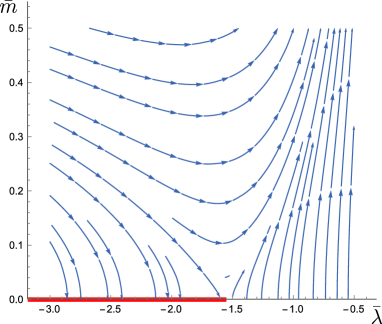
Figure 1: Flow diagrams for the RG Eqs. 51 and 52.  The red line indicates a line of fixed-points.

In order to determine the fate of the Kosterlitz-Thouless transition in the presence of the linear gradient term we make use of all the RG equations

$$\partial_{t}\bar{m}=\bar{m}+\frac{\bar{m}\bar{\lambda}}{4\pi\bar{d}^{2}}\frac{\left(1-4\bar{d}^{2}+4\bar{m}^{2}\right)}{\sqrt{\left[2\left(\frac{1-4\bar{d}^{2}+4\bar{m}^{2}}{4\bar{d}}\right)^{2}+1\right]^{2}-1}},$$ (53)

$$\partial_{t}\bar{d} =\bar{d}-\frac{\bar{\lambda}}{4\pi\bar{d}}$$

$$+\frac{\bar{\lambda}}{4\pi\bar{d}}\frac{\left(1-4\bar{d}^{2}+4\bar{m}^{2}\right)\left(1+\frac{1}{8\bar{d}^{2}}\left[1-4\bar{d}^{2}+4\bar{m}^{2}\right]\right)}{\sqrt{\left[2\left(\frac{1-4\bar{d}^{2}+4\bar{m}^{2}}{4\bar{d}}\right)^{2}+1\right]^{2}-1}},$$ (54)

$$\partial_{t}\bar{\lambda}=-\frac{2\bar{\lambda}^{2}}{\pi}\left(1-\frac{\bar{m}^{2}}{\bar{d}^{2}}\right)\frac{1}{\sqrt{\left[2\left(\frac{1-4\bar{d}^{2}+4\bar{m}^{2}}{4\bar{d}}\right)^{2}+1\right]^{2}-1}}.$$ (55)

The corresponding parametric flow is shown in Fig. 2. At finite $\bar{d}$ value, the flow is seen to initially closely follow the KT flow at $\bar{d}=0$, approach the fixed line at $\bar{m}=0$, but ultimately escape from the line toward the high-temperature phase. We may conclude that in a presence of the linear gradient term (DM interaction) no KT transition can exist.

IV Coulomb gas model

A remarkable feature found in early studies Berezinskii1971 ; Kosterlitz1973 ; Kosterlitz1974 ; Jose1977 is that the defect-mediated transition of the 2D XY model and its analogues can be mapped to the insulator-conductor transition of a two-dimensional Coulomb gas. To elucidate the origin of the flow of the Thirring model we formulate the 2D Coulomb gas model by using discrete vector calculus on a square lattice for the Hamiltonian (9), where, for simplicity, we restrict the representation by the isotropic case, $J_{||}=J_{\perp}$ . For definitness, all sums run over the sites of a square lattice although the transformation described below are easily generalized.

The partition function defined on such a lattice is of the form

$$\mathcal{Z} =\int\mathcal{D}\varphi\,\exp\biggl{[}\beta\tilde{J}\sum_{\langle ij\rangle}\cos\left(\varphi_{i}-\varphi_{j}-\alpha_{ij}\right)$$

$$\;\;\;\;+\beta h\sum_{i}\cos\varphi_{i}\biggr{]},$$ (56)

where henceforth $\beta=(k_{\text{B}}T)^{-1}$ is the inverse temperature, $\tilde{J}=S^{2}\sqrt{J^{2}+D^{2}}$ is the effective exchange parameter, $h=Sh_{x}$, and the bond angle is given by $\alpha_{ij}=\tan^{-1}\left(D/J\right)$ for the $ij$-link along the $z$-axis and zero otherwise. The first sum runs over all nearest neighbor sites within the ($xz$)-plane.

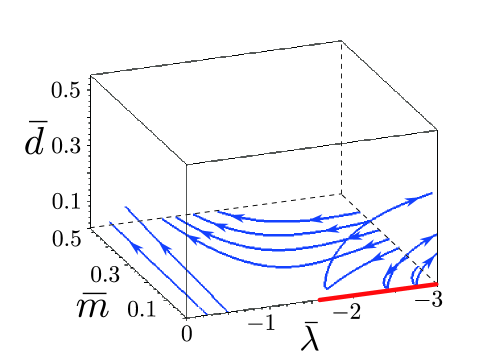
Figure 2: The RG trajectories of the 2D Thirring-like PT model. The red line indicates a line of fixed-points in the case where the linear gradient term is absent. It is seen that the flows ultimately escape from the line of fixed-points toward the high-temperature phase.

A duality mapping onto the Coulomb gas model is derived in detail in Appendix D. The resulting partition function for point charge particles reads as

$$\mathcal{Z}_{\text{eff}} =\sum_{\left\{q(\boldsymbol{r})\right\}}\,\exp\biggl{[}\pi K_{0}\sum_{\boldsymbol{r}\not=\boldsymbol{r}^{\prime}}q(\boldsymbol{r})\log\left|\boldsymbol{r}-\boldsymbol{r}^{\prime}\right|q(\boldsymbol{r}^{\prime})$$

$$\;\;\;\;+2\pi\sum_{\boldsymbol{r}}(\boldsymbol{E}_{x}\cdot\boldsymbol{r})q(\boldsymbol{r})\biggr{]}y_{0}^{\sum_{\boldsymbol{r}}\,q^{2}(\boldsymbol{r})},$$ (57)

where the bare values for the vortex coupling $K_{0}=\beta\tilde{J}$ and for the vortex pair fugacity $y_{0}=\exp\left(-\beta\pi^{2}\tilde{J}/2\right)$ . The first term in the exponential of Eq.(57) describes the charge-charge interactions, the second includes the sum of the self-energies associated with the each elementary charge $q(\boldsymbol{r})$, which arises due to the effective uniform $x$-direction field, $\boldsymbol{E}_{x}=\alpha\beta\tilde{J}\boldsymbol{e}_{x}$. The question whether a topological order realizes is thereby mapped, as in the conventional Kosterlitz-Thouless transition, to the problem of screening in the Coulomb gas, albeit now with modified terms due to the DM interaction.

The scaling equations can then be obtained from (57) in the limit of small fugacity. The procedure parallels what was detailed in Refs. Sujani1994 ; Atland2006 . At a general minimum scale $a=e^{l}$ the renormalized vortex coupling $K_{l}$, the vortex pair fugacity $y_{l}$ and the topological electric field, $\epsilon_{l}$, obey the scaling equations

$$\frac{dK_{l}}{dl} =-4\pi^{3}K_{l}^{2}y_{l}^{2},$$ (58)

$$\frac{dy_{l}}{dl} =\left(2-\pi K_{l}+\pi\epsilon_{l}\right)y_{l},$$ (59)

$$\frac{d\epsilon_{l}}{dl} =\epsilon_{l}+4\pi^{3}y_{l}^{2}K_{l}\epsilon_{l}.$$ (60)

Fig. 3. shows numerical solutions of RG flows. For $\epsilon=0$ it reproduces the well-known $K_{l}(y_{l})$ scale dependence of the KT-theory that tend asymptotically to zero (infinity) for $T>T_{\text{KT}}$, $k_{\text{B}}T_{\text{KT}}=\pi J/2$, and to constant (zero) for $T<T_{\text{KT}}$. The results for non-zero electric fields are also presented in this Figure. Apparently, at all temperatures $K_{l}$ tends asymptotically to zero and $y_{l}$ tends to infinity, i.e. vortex pairs are unbound by the electric field. It means that the breaking apart of dipoles by the topological field begins to exceed the vortex attractive interaction. In addition, the plot clearly demonstrates that the both models, the Thirring model (9) with a fictitious gauge field and the Coulomb gas in an electric field, are in the same universality class.

This concludes the RG analysis which shows that the DM interaction is relevant, it creates an effective electric field perpendicular to the direction of the DM vector on a lattice and eliminates the KT transition.

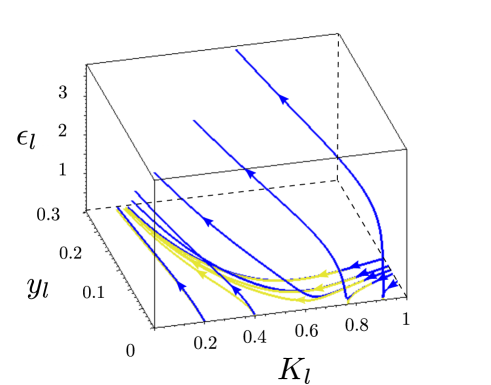
Figure 3: The RG flows of the 2D Coulomb gas counterpart of the PT model (blue) and for the XY model (yellow), $\epsilon_{l}=0$. We see that the RG flows quickly escape from the line of fixed points, which is indicated by a red line.

V Concluding remarks

In this paper we investigated the effects of the linear gradient term on a topological Kosterlitz-Thouless transition based on the functional RG approach by Wetterich. Our work has been motivated by some experimental studies on the topological defects or vortex excitations which may occur in thin films of chiral helimagnets Leonov2016 ; Fukui2016 ; Kato2017 . This class of phenomena are deeply related to the Pokrovsky-Talapov model.

Our main result is that a nonzero linear gradient term (or misfit parameter) of the PT-model, which can be related with the Dzyaloshinsky-Moriya interaction in magnetis systems, makes such a transition prohibited, what contradicts the previous consideration of this problem by the non-perturbative RG methods.

In order to argue this conclusion the initial PT model has been reformulated in terms of the 2D theory of relativistic fermions using an analogy between the 2D sine-Gordon and the massive Thirring models. In the new formalism the misfit parameter corresponds to an effective gauge field that enables to include it in the renormalization-group procedure on an equal footing with the other parameters of the theory. With the new fermionic action in hands, we apply the Wetterich equation to obtain flow equations for the parameters of the action. We demonstrate that these RG equations reproduce a KT type of behavior if the misfit equals to zero. However, any small nonzero value of the quantity rules out a possibility of the KT transition. To confirm the finding we develop a description of the issue in terms of the 2D Coulomb gas model using the corresponding mapping for the Pokrovsky-Talapov model. Within the approach the breakdown of the KT scenario gains a transparent meaning. The misfit parameter results in an appearance of an effective electric field lying in the plane what prevents a formation of bound vortex-antivortex dipoles. It is worth noting an advantage of the non-perturbative RG approach in comparison to the RG of the model of the 2D Coulomb gas. The former does not require a smallness of the magnetic field.

In closing, a matter of interest is a further application of a functional RG technique to study spin models describing a behavior of real chiral magnetic systems. In this regard we note the recent work Hering2017 , where the functional renormalization group analysis of Dzyaloshinsky-Moriya and Heisenberg spin interactions on the kagome lattice has been done.

Appendix A The inverse propagator

The matrix of second derivatives of $\Gamma_{k}$ with respect to the fermion fields deduced from Eq.(14)

$$\Gamma_{k}^{(2)}(p,q)=\left(\begin{array}[c]{cc}\overrightarrow{\partial}_{\psi_{-p}^{T}}\Gamma_{k}\overleftarrow{\partial}_{\psi_{q}}&\overrightarrow{\partial}_{\psi_{-p}^{T}}\Gamma_{k}\overleftarrow{\partial}_{\bar{\psi}_{-q}^{T}}\\ \overrightarrow{\partial}_{\bar{\psi}_{p}}\Gamma_{k}\overleftarrow{\partial}_{\psi_{q}}&\overrightarrow{\partial}_{\bar{\psi}_{p}}\Gamma_{k}\overleftarrow{\partial}_{\bar{\psi}_{-q}^{T}}\end{array}\right)$$ (61)

results in the field-independent part

$$\Gamma_{k,0}^{(2)}(p,q)=\frac{\delta_{p,q}}{(2\pi)^{2}}$$

$$\times\left(\begin{array}[c]{cc}0&\begin{array}[c]{c}-Z_{k}\not{p}^{T}\\ +i\not{d}^{T}-i\tilde{m}\end{array}\\ \begin{array}[c]{c}-Z_{k}\not{p}\\ -i\not{d}+i\tilde{m}\end{array}&0\end{array}\right).$$ (68)

Then the inverted form of the regularized propagator reads

$$\left(\Gamma_{k,0}^{(2)}+R_{k}\right)(p,q)=\frac{\delta_{p,q}}{(2\pi)^{2}}$$

$$\times\left(\begin{array}[c]{cc}0&\begin{array}[c]{c}-Z_{k}\not{p}^{T}\left[1+r\left(\frac{q^{2}}{k^{2}}\right)\right]\\ +i\not{d}^{T}-i\tilde{m}\end{array}\\ \begin{array}[c]{c}-Z_{k}\not{p}\left[1+r\left(\frac{q^{2}}{k^{2}}\right)\right]\\ -i\not{d}+i\tilde{m}\end{array}&0\end{array}\right),$$ (75)

the inverse of the matrix yields the result (21). To find the form of the field-dependent part (25) the property $\bar{\psi}\psi=-\psi^{T}\bar{\psi}^{T}$ appears to be useful.

Appendix B Treshold functions

The flow equations include single integrals due to one-loop structure of Wetterich equation, the threshold functions, which contain details of the regularization scheme. The definitions of the threshold functions are given by Eqs.(31,32,41). In the flow equations $\tilde{\partial}_{k}$ is defined to act on the regulator’s $k$-dependence. The sharp cut-off regulator (42) has the remarkable feature that all threshold integrals can be done explicitly.

Indeed, in the polar coordinates

$$\tilde{\partial}_{k}\mathcal{L}_{1}$$

$$=\tilde{\partial}_{k}\int_{k}^{\Lambda}\frac{dq}{(2\pi)^{2}}\int_{0}^{2\pi}d\phi\frac{q\left(q^{2}-d_{k}^{2}+\tilde{m}_{k}^{2}\right)}{\left(q^{2}-d_{k}^{2}+\tilde{m}_{k}^{2}\right)^{2}+4d_{k}^{2}q^{2}\cos^{2}\phi},$$ (76)

where $\Lambda$ is the ultraviolet cutoff, and we take into account that $a=-1$ for the regulator (42).

The needed dependence on $k$ appears only in the lower limit of the integration over $q$. Therefore, we obtain

$$k\tilde{\partial}_{k}\mathcal{L}_{1} =-\frac{1}{8\pi^{2}}\frac{\left(k^{2}-d_{k}^{2}+\tilde{m}_{k}^{2}\right)}{d^{2}}$$

$$\times\int_{0}^{2\pi}\frac{d\phi}{2\left(\frac{k^{2}-d_{k}^{2}+\tilde{m}_{k}^{2}}{2kd_{k}}\right)^{2}+1+\cos 2\phi}.$$ (77)

Once the simple integration is performed, we get

$$k\tilde{\partial}_{k}\mathcal{L}_{1}$$

$$=-\frac{\left(k^{2}-d_{k}^{2}+\tilde{m}_{k}^{2}\right)}{4\pi d_{k}^{2}}\frac{1}{\sqrt{\left[2\left(\frac{k^{2}-d_{k}^{2}+\tilde{m}_{k}^{2}}{2kd_{k}}\right)^{2}+1\right]^{2}-1}}.$$ (78)

Similarly, the scale derivative of $\mathcal{L}_{2}$ is given by

$$k\tilde{\partial}_{k}\mathcal{L}_{2}=\left[1+\frac{1}{2d^{2}}\left(k^{2}-d^{2}+\tilde{m}^{2}\right)\right]k\tilde{\partial}_{k}\mathcal{L}_{1}+\frac{k^{2}}{4\pi d^{2}}.$$ (79)

To find the RG running of $\mathcal{L}_{3}$ we first note that

$$\text{det}\left(\frac{\not{\alpha}_{k}-i\tilde{m}_{k}}{\alpha_{k}^{2}+\tilde{m}_{k}^{2}}\right) =-\frac{1}{\alpha_{k}^{2}+\tilde{m}_{k}^{2}},$$ (80)

$$\text{det}\left(\frac{\not{\beta}_{k}+i\tilde{m}_{k}}{\beta_{k}^{2}+\tilde{m}_{k}^{2}}\right) =-\frac{1}{\beta_{k}^{2}+\tilde{m}_{k}^{2}},$$ (81)

and

$$\mathcal{X}\left(\frac{\not{\alpha}_{k}-i\tilde{m}_{k}}{\alpha_{k}^{2}+\tilde{m}_{k}^{2}},\frac{\not{\beta}_{k}+i\tilde{m}_{k}}{\beta_{k}^{2}+\tilde{m}_{k}^{2}}\right)$$

$$=\frac{\tilde{m}_{k}^{2}-\alpha_{1k}\beta_{1k}-\alpha_{2k}\beta_{2k}}{\left(\alpha_{k}^{2}+\tilde{m}_{k}^{2}\right)\left(\beta_{k}^{2}+\tilde{m}_{k}^{2}\right)}.$$ (82)

Therefore,

$$\ -\text{det}\left(\frac{\not{\alpha}_{k}-i\tilde{m}_{k}}{\alpha_{k}^{2}+\tilde{m}_{k}^{2}}\right)-\text{det}\left(\frac{\not{\beta}_{k}-i\tilde{m}_{k}}{\beta_{k}^{2}+\tilde{m}_{k}^{2}}\right)$$

$$+2\mathcal{X}\left(\frac{\not{\alpha}_{k}-i\tilde{m}_{k}}{\alpha_{k}^{2}+\tilde{m}_{k}^{2}},\frac{\not{\beta}_{k}+i\tilde{m}_{k}}{\beta_{k}^{2}+\tilde{m}_{k}^{2}}\right)$$

$$=\frac{4\tilde{m}_{k}^{2}+\left(\alpha_{1k}-\beta_{1k}\right)^{2}+\left(\alpha_{2k}-\beta_{2k}\right)^{2}}{\left(\alpha_{k}^{2}+\tilde{m}_{k}^{2}\right)\left(\beta_{k}^{2}+\tilde{m}_{k}^{2}\right)}.$$ (83)

For the sharp cutoff (42), for which $\alpha_{1k}-\beta_{1k}=-2id_{k}$ and $\alpha_{2k}-\beta_{2k}=0$, the last expression reads

$$\frac{4\left(\tilde{m}_{k}^{2}-d_{k}^{2}\right)}{\left(q^{2}-d_{k}^{2}+\tilde{m}_{k}^{2}\right)^{2}+4q_{1}^{2}d_{k}^{2}}.$$ (84)

Through the insertion of the result into Eq.(41) we obtain

$$\mathcal{L}_{3}=\frac{1}{\pi^{2}}\int_{k}^{\Lambda}dq\,q\int_{0}^{2\pi}d\phi\,\frac{\left(\tilde{m}_{k}^{2}-d_{k}^{2}\right)}{\left(q^{2}-d_{k}^{2}+\tilde{m}_{k}^{2}\right)^{2}+4q^{2}d_{k}^{2}\cos^{2}\phi}.$$ (85)

From the definition it follows that

$$k\tilde{\partial}_{k}\mathcal{L}_{3}=\frac{4\left(\tilde{m}^{2}_{k}-d^{2}_{k}\right)}{\left(k^{2}-d^{2}_{k}+\tilde{m}^{2}_{k}\right)^{2}}k\,\tilde{\partial}_{k}\mathcal{L}_{1}.$$ (86)

Appendix C Canonical dimensions

We discuss the dimensionality of the various quantities introduced. The lengths, $x$, have dimensions $[x]=-1$ , i.e. the dimension of inverse momenta. The dimension of the spinor fields, $\bar{\psi}$, $\psi$, follows from inspection of the standard kinetic term, $\int d^{D}x\,\bar{\psi}\partial_{x}\psi$. Since this is a contribution to the action it must be dimensionless that yields

$$\left[\bar{\psi}\right]=\left[\psi\right]=\frac{1}{2}\left(D-1\right).$$ (87)

For the same reason $[m]=1$, $[d]=1$ and $[\lambda]=2-D$.

Appendix D The electrostatic model

To introduce the duality mapping we replace Nagaosa in the partition function (56)

$$e^{\beta\tilde{J}\cos\Phi_{ij}}\rightarrow e^{\beta\tilde{J}}\sum_{m=-\infty}^{m=+\infty}\exp\left[-\frac{\beta\tilde{J}}{2}\left(\Phi_{ij}-2\pi m\right)^{2}\right],$$ (88)

where $\Phi_{ij}=\varphi_{i}-\varphi_{j}-\alpha_{ij}$, and use the Poisson sum formula which states

$$\sum_{m=-\infty}^{+\infty}f(m)=\sum_{l=-\infty}^{+\infty}\int_{-\infty}^{+\infty}d\phi\,f(\phi)e^{2\pi il\phi}.$$ (89)

This yields

$$e^{\beta\tilde{J}\cos\Phi_{ij}}$$

$$\rightarrow\frac{1}{\sqrt{2\pi\beta\tilde{J}}}\sum_{l_{ij}=-\infty}^{+\infty}e^{\beta\tilde{J}}\exp\left[-\frac{l_{ij}^{2}}{2\beta\tilde{J}}+il_{ij}\Phi_{ij}\right].$$ (90)

After substitution the result into (56) and omitting nonessential factors we get

$$\mathcal{Z} =\int\mathcal{D}\varphi\,\sum_{\left\{l_{ij}\right\}}\exp\biggl{(}-\sum_{\langle ij\rangle}\left[\frac{l_{ij}^{2}}{2\beta\tilde{J}}-il_{ij}\Phi_{ij}\right]$$

$$\;\;\;\;+\beta h\sum_{i}\cos\varphi_{i}\biggr{)}.$$ (91)

We now define a vector field $l_{\mu}(\boldsymbol{r})$ ($\mu=1,2$) that is directed from the starting point $\boldsymbol{r}$, which is the left-hand side or lower side of the link between the sites $i$ and $j$, to the other side of the link. The vector field takes the value $l_{ij}$ on the link. The partition function is then just the sum over all possible values $l_{\mu}(\boldsymbol{r})$ of the form

$$\mathcal{Z} =\sum_{\left\{l_{\mu}(\boldsymbol{r})\right\}}\int\mathcal{D}\varphi\,\exp\biggl{(}-\sum_{\boldsymbol{r},\mu}\biggl{[}\frac{l_{\mu}^{2}(\boldsymbol{r})}{2\beta\tilde{J}}$$

$$-il_{\mu}(\boldsymbol{r})\left\{\varphi(\boldsymbol{r})-\varphi(\boldsymbol{r}+\boldsymbol{a}_{\mu})\right\}+il_{\mu}(\boldsymbol{r})\alpha_{\mu}\biggr{]}$$

$$+\beta h\sum_{\boldsymbol{r}}\cos\varphi(\boldsymbol{r})\biggr{)},$$ (92)

where $\alpha_{\mu}$ coincides with $\alpha_{ij}$ on the $ij$-link, and $\boldsymbol{a}_{\mu}$ is the lattice unit.

To evaluate the sum we shall make use

$$\sum_{\boldsymbol{r},\mu}l_{\mu}(\boldsymbol{r})\left\{\varphi(\boldsymbol{r})-\varphi(\boldsymbol{r}+\boldsymbol{a}_{\mu})\right\}$$

$$=\sum_{\boldsymbol{r},\mu}\left\{l_{\mu}(\boldsymbol{r})-l_{\mu}(\boldsymbol{r}-\boldsymbol{a}_{\mu})\right\}\varphi(\boldsymbol{r})$$ (93)

to transform the partition function into

$$\mathcal{Z} =\sum_{\left\{l_{\mu}(\boldsymbol{r})\right\}}\int\mathcal{D}\varphi\,\exp\biggl{(}-\sum_{\boldsymbol{r},\mu}\biggl{[}\frac{l_{\mu}^{2}(\boldsymbol{r})}{2\beta\tilde{J}}$$

$$-i\left\{l_{\mu}(\boldsymbol{r})-l_{\mu}(\boldsymbol{r}-\boldsymbol{a}_{\mu})\right\}\varphi(\boldsymbol{r})+il_{\mu}(\boldsymbol{r})\alpha_{\mu}\biggr{]}$$

$$+\beta h\sum_{\boldsymbol{r}}\cos\varphi(\boldsymbol{r})\biggr{)}.$$ (94)

We wish to perform integration over $\varphi(\boldsymbol{r})$ from $0$ to $2\pi$. The goal is easily accomplished with the aid of the Jacobi-Anger expansion

$$e^{z\cos\varphi}=I_{0}(z)+2\sum_{k=1}^{\infty}I_{k}(z)\cos(k\varphi),$$ (95)

where $I_{k}(z)$ is the modified Bessel function of the first kind.

The $\varphi$ integrals can be then done immediately that reduces the partition function to a sum over the bond variables $l_{\mu}(\boldsymbol{r})$ with a set of $\delta$-functions restricting these variables at every site

$$\mathcal{Z} \propto\sum_{\left\{l_{\mu}(\boldsymbol{r})\right\}}\exp\left[-\sum_{\boldsymbol{r}\mu}\left(\frac{l_{\mu}^{2}(\boldsymbol{r})}{2\beta\tilde{J}}+il_{\mu}(\boldsymbol{r})\alpha_{\mu}\right)\right]$$

$$\times\prod_{\boldsymbol{r}}\biggl{[}\sum_{\kappa(\boldsymbol{r})=-\infty}^{\infty}I_{\kappa(\boldsymbol{r})}(\beta h)$$

$$\times\delta\left[\sum_{\mu}\left(l_{\mu}(\boldsymbol{r})-l_{\mu}(\boldsymbol{r}-\boldsymbol{a}_{\mu})\right)-\kappa(\boldsymbol{r})\right]\biggr{]}.$$ (96)

A presence of the magnetic field violates the ”zero divergence” condition,

$$\sum_{\mu}\left(l_{\mu}(\boldsymbol{r})-l_{\mu}(\boldsymbol{r}-\boldsymbol{a}_{\mu})\right)=0,$$ (97)

giving the effective integer-valued charges $\kappa(\boldsymbol{r})$ confined to lattice sites.

To gain an insight into the nature of the constraints imposed by the $\delta$-functions it is worthy of note that $l_{\mu}(\boldsymbol{r})$ can be split into the longitudinal and transverse parts Polyakov

$$l_{\mu}(\boldsymbol{r}) =m(\boldsymbol{r})-m(\boldsymbol{r}+\boldsymbol{a}_{\mu})+\sigma(\boldsymbol{r})-\sigma(\boldsymbol{r}+\boldsymbol{a}_{\mu})$$

$$+\varepsilon_{\mu\nu}\left[n(\boldsymbol{r})-n(\boldsymbol{r}-\boldsymbol{a}_{\nu})\right],$$ (98)

where $\varepsilon_{\mu\nu}$ is the standard antisymmetric tensor, the $m(\boldsymbol{r})$ and $n(\boldsymbol{r})$ are integers, $|\sigma(\boldsymbol{r})|<1$.

The transversal vector field $\boldsymbol{n}(\boldsymbol{r})=n(\boldsymbol{r})\boldsymbol{e}_{3}$, where $\boldsymbol{e}_{3}$ is perpendicular to the plane of the system, realizes the discrete version of the equation $\boldsymbol{l}(\boldsymbol{r})=\text{rot}\,\boldsymbol{n}(\boldsymbol{r})$,

$$\begin{array}[c]{c}l_{1}(\boldsymbol{r})=n(\boldsymbol{r})-n(\boldsymbol{r}-\boldsymbol{a}_{2}),\\ l_{2}(\boldsymbol{r})=-n(\boldsymbol{r})+n(\boldsymbol{r}-\boldsymbol{a}_{1}),\end{array}$$ (99)

that ensure that the ”zero divergence” condition (97) is properly satisfied.

The $\delta$-function condition in Eq.(96) can, in turn, be satisfied if the longitudinal part obeys the discrete Poisson equation

$$-\sum_{\mu}[m(\boldsymbol{r}+\boldsymbol{a}_{\mu})+m(\boldsymbol{r}-\boldsymbol{a}_{\mu})-2m(\boldsymbol{r})$$

$$+\sigma(\boldsymbol{r}+\boldsymbol{a}_{\mu})+\sigma(\boldsymbol{r}-\boldsymbol{a}_{\mu})-2\sigma(\boldsymbol{r})]=\kappa(\boldsymbol{r}).$$ (100)

Here, the $m(\boldsymbol{r})$ are required to be integer-valued and $\sigma(\boldsymbol{r})$ are adjusted to keep Eq. (100).

Given that we are primary focusing on a role of the DM interaction we restrict ourselves to the case of vanishing magnetic fields, $\beta h\to 0$, when $I_{\kappa(\boldsymbol{r})}(\beta h)$ can be replaced by the delta symbol $\delta_{\kappa,0}$ and the trivial solution $m(\boldsymbol{r})+\sigma(\boldsymbol{r})=0$ can be taken for Eq.(100).

By substituting (99) in Eq.(96) and taking account of $\alpha_{\mu}=\alpha\delta_{\mu,1}$ we find

$$\mathcal{Z} =\sum_{\left\{n(\boldsymbol{r})\right\}}\exp\biggl{[}-\sum_{\boldsymbol{r}\mu}\frac{1}{2\beta\tilde{J}}\left\{n(\boldsymbol{r})-n(\boldsymbol{r}-\boldsymbol{a}_{\mu})\right\}^{2}$$

$$-i\alpha\sum_{\boldsymbol{r}}\left\{n(\boldsymbol{r})-n(\boldsymbol{r}-\boldsymbol{a}_{2})\right\}\biggr{]}.$$ (101)

Rewriting the sum running over integers $n(\boldsymbol{r})$ through the Poisson formula (89) one obtain

$$\mathcal{Z} =\int\mathcal{D}\phi\,\sum_{\left\{q(\boldsymbol{r})\right\}}\,\exp\biggl{[}-\frac{1}{2\beta\tilde{J}}\sum_{\boldsymbol{r},\mu}\left(\hat{\Delta}_{\mu}\phi\right)^{2}$$

$$-i\alpha\sum_{\boldsymbol{r}}\hat{\Delta}_{2}\phi+2\pi i\sum_{\boldsymbol{r}}q(\boldsymbol{r})\phi(\boldsymbol{r})\biggr{]},$$ (102)

where the lattice difference is defined as $\hat{\Delta}_{\mu}\phi(\boldsymbol{r})=\phi(\boldsymbol{r})-\phi(\boldsymbol{r}-\boldsymbol{a}_{\mu})$.

Making use of the parallel translation in the functional space Yaglom1960 , $\phi(\boldsymbol{r})\rightarrow\phi(\boldsymbol{r})-i\alpha\beta\tilde{J}x_{2}$, and carrying out Gaussian integration over $\phi(\boldsymbol{r})$ we are led to

$$\mathcal{Z}_{\text{eff}} \propto\sum_{\left\{q(\boldsymbol{r})\right\}}\exp\biggl{[}-2\pi^{2}\beta\tilde{J}\sum_{\boldsymbol{r},\boldsymbol{r}^{\prime}}q(\boldsymbol{r})G(\boldsymbol{r}-\boldsymbol{r}^{\prime})q(\boldsymbol{r}^{\prime})$$

$$+2\pi\alpha\beta\tilde{J}\sum_{\boldsymbol{r}}q(\boldsymbol{r})\,x_{2}\biggr{)}.$$ (103)

The lattice Green function takes the form Jose1977

$$G\left(\boldsymbol{r}-\boldsymbol{r}^{\prime}\right) =\int\frac{d^{2}k}{(2\pi)^{2}}\,\frac{e^{i\boldsymbol{k}\cdot\left(\boldsymbol{r}-\boldsymbol{r}^{\prime}\right)}}{4-2\cos k_{x}-2\cos k_{y}}$$

$$\approx-\frac{1}{2\pi}\ln\left(\frac{\left|\boldsymbol{r}-\boldsymbol{r}^{\prime}\right|}{a}\right)-\frac{1}{4}+G(0),$$ (104)

where the last term does not contain divergent terms. Interpreting $q(\boldsymbol{r})$ as an electric charge at the position $\boldsymbol{r}$ and the logarithmic potential as the Coulomb potential in two dimensions, the term with $G(0)$ disappears if the charge neutrality condition, $\sum_{\boldsymbol{r}}q(\boldsymbol{r})=0$, is imposed. The remaining part of $G\left(\boldsymbol{r}-\boldsymbol{r}^{\prime}\right)$ leads to the result (57).

References

• (1) V.L. Pokrovsky and A.L. Talapov, Phys. Rev. Lett. 42, 65 (1979).
• (2) V.L. Pokrovsky and A.L. Talapov, Zh. Eksp. Teor. Fiz. 78, 269 (1980) [Sov. Phys. JETP 51, 134 (1980)].
• (3) K. Yang, K. Moon, L. Belkhir, H. Mori, S.M. Girvin, and A.H. MacDonald, Phys. Rev. B 54, 11644 (1996).
• (4) T. Dröse, R. Besseling, P. Kes, P. and Morais C. Smith, Phys. Rev. B 67, 064508 (2003).
• (5) H.P. Blücher, G. Blatter and W. Zwerger, Phys. Rev. Lett. 90, 130401 (2003).
• (6) R.A. Molina, J. Dukelsky and P. Schmitteckert, Phys. Rev. Lett. 99, 080404 (2007).
• (7) C. R. Woods, L. Britnell, A. Eckmann, R.S. Ma, J.C. Lu, H.M. Guo, X. Lin, G.L. Yu, Y. Cao, R.V. Gorbachev, A.V. Kretinin, J. Park, L.A. Ponomarenko, M.I. Katsnelson, Yu.N. Gornostyrev, K. Watanabe, T. Taniguchi, C. Casiraghi, H-J. Gao, A.K. Geim, K.S. Novoselov, 10, 451 (2014).
• (8) P. Bak, Rep. Prog. Phys. 45, 587 (1982).
• (9) I.E. Dzyaloshinskii, JETP 19, 960 (1964).
• (10) J. Heurich, J. König and A.H. MacDonald, Phys. Rev. B 68, 064406 (2003).
• (11) J. Kishine, I.G. Bostrem, A.S. Ovchinnikov and Vl.E. Sinitsyn, Phys. Rev. B 89, 014419 (2014).
• (12) Molecule surface interactions, Ed. by K.P. Lawley, Adv. in Chem. Physics, Vol. 76 (1989).
• (13) S.N. Coppersmith, D.S. Fisher, B.I. Halperin, P.A. Lee and W.F. Brinkman, Phys. Rev. Lett. 46, 549 (1981); Phys. Rev. B 25, 349 (1982).
• (14) J.M. Kosterlitz and D.J. Thouless, J. Phys. C: Solid State Phys. 6, 1181 (1973).
• (15) Y. Togawa, T. Koyama, K. Takayanagi, S. Mori, Y. Kousaka, J. Akimitsu, S. Nishihara, K. Inoue, A. S. Ovchinnikov, and J. Kishine, Phys. Rev. Lett. 108, 107202 (2012).
• (16) Y. Togawa, T. Koyama, Y. Nishimori, Y. Matsumoto, S. McVitie, D. McGrouther, R. L. Stamps, Y. Kousaka, J. Akimitsu, S. Nishihara, K. Inoue, I. G. Bostrem, Vl. E. Sinitsyn, A. S. Ovchinnikov, and J. Kishine Phys. Rev. B 92, 220412(R) (2015).
• (17) F. J. T. Goncalves, T. Sogo, Y. Shimamoto, Y. Kousaka, J. Akimitsu, S. Nishihara, K. Inoue, D. Yoshizawa, M. Hagiwara, M. Mito, R. L. Stamps, I. G. Bostrem, V. E. Sinitsyn, A. S. Ovchinnikov, J. Kishine, and Y. Togawa Phys. Rev. B 95 104415 (2017)
• (18) J. Kishine and A. Ovchinnikov, Solid State Phys. 66, 1 (2015).
• (19) M.W. Puga, E. Simanek, and H. Beck, Phys. Rev. D 26, 2673 (1982).
• (20) B. Horowitz, T. Bohr, J.M. Kosterlitz and H.J. Schulz, Phys. Rev. B 28, 6596 (1983).
• (21) V.L. Berezinskii, Sov. Phys. JETP 32, 493 (1971).
• (22) J.M. Kosterlitz, J. Phys. C: Solid State Phys. 7, 1046 (1974).
• (23) J.V. José, L. P. Kadanoff, S. Kirkpatrick, and D. R. Nelson, Phys. Rev. B 16, 1217 (1977).
• (24) A. Lazarides, O. Tieleman, and C. Morrais Smith, Phys. Rev. B 80, 245418 (2009).
• (25) C. Wetterich, Phys. Lett. B 301, 90 (1993).
• (26) J. Berges, N. Tetradis and C. Wetterich, Phys. Rept. 363, 223 (2002).
• (27) G. v. Gersdorff and C. Wetterich, Phys. Rev. B 64, 054513 (2001).
• (28) P. Jakubczyk, N. Dupuis, B. Delamotte, Phys. Rev. E 90, 062105 (2014).
• (29) M. Gräter and C. Wetterich, Phys. Rev. Lett. 75, 378 (1995).
• (30) S. Nagy, I. Nándory, J. Polonyi and K. Sailer, Phys. Rev. Lett. 102, 241603 (2009).
• (31) N. Nagaosa, Quantum Fiedl Theory in Condensed Matter Physics, Springer, 1999.
• (32) S. Coleman, Phys. Rev. D 11, 2088 (1975).
• (33) S. Mandelstam, Phys. Rev. D 11, 3026 (1975).
• (34) W. Metzner, M. Salmhofer, C. Honerkamp, V. Meden, Rev. Mod. Phys. 84, 299 (2012).
• (35) P. Kopietz and T. Busche, Phys. Rev. B 64, 155101 (2001).
• (36) A. Luther and I. Peschel, Phys. Rev. B 12, 3908 (1975).
• (37) E. Witten, Comm. Math. Phys. 92, 455 (1984).
• (38) H. Gies and L. Janssen, Phys. Rev. D 82, 085018 (2010).
• (39) L.P. Kadanoff, J. Phys. A: Math. Gen. 11, 1399 (1978).
• (40) C.E.I. Carneiro, J.A. Mignaco, M.T. Thomaz, Phys. Rev. D 36, 1282 (1987).
• (41) J. Braun, Journal of Physics G: Nuclear and Particle Physics 39, 033001 (2012).
• (42) K. Yoshida, unpublished, arxiv:hep-th/0204086.
• (43) S. Sujani, B. Chattopadhyay and S.R. Shenoy, Phys. Rev. B 50, 16668 (1994).
• (44) A. Atland and B. Simons, Condensed Matter Field Theory, Cambridge University Press, 2006.
• (45) A.M. Polyakov, Gauge Fields and Strings, Taylor & Francis, 1987.
• (46) I.M. Gel’fand and A.M. Yaglom, J. Math. Phys. 1, 48 (1960).
• (47) S. Nagy, I. Nándory, J. Polonyi and K. Sailer, Phys. Rev. D 77, 025026 (2008).
• (48) A. O. Leonov, Y. Togawa, T. L. Monchesky, A. N. Bogdanov, J. Kishine, Y. Kousaka, M. Miyagawa, T. Koyama, J. Akimitsu, Ts. Koyama, K. Harada, S. Mori, D. McGrouther, R. Lamb, M. Krajnak, S. McVitie, R. L. Stamps, and K. Inoue, Phys. Rev. Lett. 117, 087202 (2016).
• (49) S. Fukui, M. Kato and Y. Togawa, Supercond. Sci. Technol. 29, 125008 (2016).
• (50) M. Kato, S. Fukui, O. Sato and Y. Togawa, Physica C 533, 137 (2017).
• (51) M. Hering and J. Reuther, Phys. Rev. B 95, 054418 (2017).