Randomly cross-linked polymer models

Abstract

Polymer models are used to describe chromatin, which can be folded at different spatial scales by binding molecules. By folding, chromatin generates loops of various sizes. We present here a randomly cross-linked (RCL) polymer model, where monomer pairs are connected randomly. We obtain asymptotic formulas for the steady-state variance, encounter probability, the radius of gyration, instantaneous displacement and the mean first encounter time between any two monomers. The analytical results are confirmed by Brownian simulations. Finally, the present results can be used to extract the minimum number of cross-links in a chromatin region from conformation capture data.

DNA in the nucleus is constantly remodeled by regulatory factors and compacted genomic regions form transient and stable loops Nora et al. (2012); Tark-Dame et al. (2014). Looping is thus a key event in chromatin regulation: it is rare for a single polymer but frequent in a population of hierarchy folded genome. Genome organization is now probed by chromatin Conformation Capture (CC) techniques Dekker et al. (2002); Simonis et al. (2006); Lieberman-Aiden et al. (2009), which simultaneously give access to looping events in an ensemble of millions of chromatin segments. This experimental approach provides contact frequency matrices at various scale from few kilo- to Mega-base-pairs. Analysis of these matrices remains difficult, but revealed that mammalian genomes contain ”blocks” of up to few Mbp in size, called Topologically Associating Domains (TADs) Nora et al. (2012); Dixon et al. (2012). The role of TADs and organization remains unclear, although they are involved in gene regulation Nora et al. (2012); Simonis et al. (2006) and replication. TADs appear by averaging encounters over an ensemble of millions of samples Lieberman-Aiden et al. (2009) and represents steady-state looping frequencies, but does not contain neither directly information about the size of the folded genomic section nor any transient genomic encounter times.
To reconstruct chromatin at a given scale and explore its transient properties, polymer models are used as a coarse-grained representation. The Rouse model Doi and Edwards (1986), characterized by nearest neighbors interactions, predicts an encounter probability (EP) that decays with $|m-n|^{-3/2}$ between monomer $m$ and $n$, but cannot account for long-range interactions, observed inside TADs of the CC data Shukron and Holcman (2017); Nora et al. (2012). Other polymer models include attractive and repulsive forces between monomers Sokolov (2003); Bohn et al. (2007); Bohn and Heermann (2010); Heermann (2011); Amitai and Holcman (2013); Langowski and Heermann (2007) to account for long-range interactions and have been used to probe the heterogeneous steady-state organization of the chromatin, characterized by loops Jost et al. (2014).
We study here a randomly cross-linked (RCL) polymer model used in Shukron and Holcman (2017) to describe the ensemble of chromatin conformation, where random cross-links are formed by binding molecules Nora et al. (2012). The space of RCL polymer configurations was so far explored only numerically Heermann (2011); Jespersen et al. (2000), but no analytical formulas have been derived for studying the steady-state or transient properties and thus explore the large parameter space. We derive here novel analytical formulas for the encounter probability (EP), variance, and the radius of gyration of the RCL polymer, that we use to study the polymer dynamics. The present model can be used to determine from CC empirical EP , the minimal number of cross-links, inaccessible from CC experiments. We further study the mean first encounter time between any two monomers, which plays a key role in gene regulation Kadauke and Blobel (2009). Most of the asymptotic derivations are confirmed by Brownian simulations.
The RCL polymer model. We start with a linear polymer in dimension $d(d=3)$ consisting of $N$ monomers with positions $R=[r_{1},r_{2},...,r_{N}]^{T}$, connected sequentially by harmonic springs Doi and Edwards (1986) and we added connectors between random non-nearest neighboring (NN) monomer pairs (Fig. 1A). The potential energy of the RCL polymer is the sum of the spring potential of linear backbone and that of random connectors

$$\phi(R)=\frac{\kappa}{2}\sum^{N}_{n=2}(r_{n}-r_{n-1})^{2}+\frac{\kappa}{2}\sum_{\mathcal{G}}(r_{m}-r_{n})^{2},$$ (1)

where $\kappa=dk_{B}T/b^{2}$ is the spring constant, $b$ the standard-deviation of the connector between connected monomers, $k_{B}$ is the Boltzmann’s constant and $T$ the temperature. The ensemble $\mathcal{G}$ is composed of $N_{c}$ randomly chosen indices $m,n$ among the non-NN monomers. We define the connectivity fraction $0\leq\xi\leq 1$, as the fraction of connector numbers $N_{L}=\frac{(N-1)(N-2)}{2}$,

$$N_{c}(\xi)=\lfloor\xi N_{L}\rfloor.$$ (2)

For each polymer realization, we choose $N_{c}$ pairs from the possible $N_{L}$ NN monomers. The dynamics of the resulting polymer monomers (vector $R$) is driven by Brownian motion and the field of force due to the potential energy 1, leading to the stochastic description

$$\frac{d\mbox{\boldmath$R$}}{dt}=-\frac{d}{b^{2}}D\left(M+B(\xi)\right)\mbox{\boldmath$R$}+\sqrt{2D}\frac{d\mbox{\boldmath$\omega$}}{dt},$$ (3)

where $D=\frac{k_{B}T}{\zeta}$ is the diffusion constant, $\zeta$ is the friction coefficient, $\omega$ are independent white noise with mean 0 and variance 1, $M$ is the $N\times N$ Rouse matrix Doi and Edwards (1986)

$$M_{m,n}=\begin{cases}-\sum_{j\neq m}M_{m,j},&m=n;\\ -1&|m-n|=1;\\ 0,&\text{otherwise}.\end{cases}$$ (4)

For a given $\xi$, the square symmetric matrix $B(\xi)$ with random connectivity is defined by

$$B_{mn}(\xi)=\begin{cases}-1,&|m-n|>1,\text{and connected};\\ -\sum_{i\neq j}^{N}B_{mj}(\xi),&m=n;\\ 0,&\text{ otherwise.}\end{cases}$$

To derive the steady-state properties of an ensemble of RCL polymers, we adopt a mean-field model where we replace the matrix $B(\xi)$ in Eq. 3 by its average $\langle B(\xi)\rangle$ (averaging over all configurations of non NN connected monomer pairs). We thus construct $\langle B(\xi)\rangle$, using the probability density of the monomer connectivity. For a fixed number of connector $N_{c}$, the probability that monomer $m$ has $k\leq(N-2)$ non-NN connections is obtained by choosing $k$ position in row $m$ of the matrix $B(\xi)$ (excluding the super- and sub- and the diagonal), and the remaining $Nc-k$ connectors in any row or column $n\neq m$:

$$Pr_{m}(k)=\begin{cases}\frac{C^{N_{c}(\xi)-k}_{N_{L}-(N-3)}C^{k}_{N-3}}{C^{N_{c}(\xi)}_{N_{L}}},&1<m<N;\\ \frac{C^{N_{c}(\xi)-k}_{N_{L}-(N-2)}C^{k}_{N-2}}{C^{N_{c}(\xi)}_{N_{L}}},&m=1,N,\end{cases}$$ (5)

where the binomial coefficient is $C_{i}^{j}=\frac{i!}{(i-j)!j!}$. This probability is the hyper-geometric distribution for the number of connections for monomer $m$. The mean number of connectors for each monomer is therefore

$$\beta_{m}(\xi)=\begin{cases}\frac{(N-3)N_{c}(\xi)}{N_{L}}\approx(N-3)\xi,&1<m<N;\\ \frac{(N-2)N_{c}(\xi)}{N_{L}}\approx(N-2)\xi,&m=1,N.\end{cases}$$ (6)

Using the mean values in 6, we obtain the expression for the matrix $\langle B(\xi)\rangle$, with entries

$$\langle B_{mn}(\xi)\rangle=\begin{cases}-\xi,&|m-n|>1;\\ \beta_{m}(\xi),&m=n;\\ 0,&\text{otherwise},\\ \end{cases}$$ (7)

which can be decomposed as the sum

$$\langle B(\xi)\rangle=\xi(N\mbox{\boldmath$I_{d}$}-\mbox{\boldmath$M$}-\mbox{\boldmath$1$}_{N}),$$ (8)

where $I_{d}$ is the $N\times N$ identity matrix, and $\mbox{\boldmath$1$}_{N}$ is a $N\times N$ matrix of ones. To study the mean properties of the RCL polymer, we study the stochastic process 3 using the average matrix $\langle B(\xi)\rangle$.

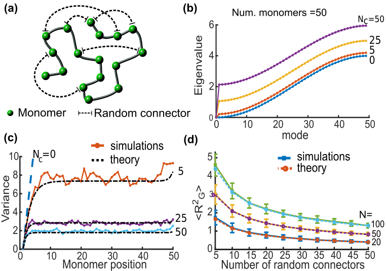
Figure 1: Steady-state properties of a Randomly-Cross-Linked (RCL) polymer. (a) representation of a RCL polymer composed of a linear backbone of $N$ monomers (spheres), and $N_{c}$ random connectors (dashed) between non-nearest neighboring monomers pairs. (b) Eigenvalues of the RCL polymer (Eq. 16) with $N=50$ monomers, and $N_{c}=5$ (blue), 25 (red), and 50 (yellow) connectors. (c) Variance of the monomers’ distance: analytical (dashed, Eq.25) versus simulated (Eq.13) between monomer 1 and monomers 2-50 of the RCL polymer, 500 realizations with $N=50,b=\sqrt{d},D=1,\Delta t=0.01s$, for $N_{c}=5$ (blue), 25 (yellow) and 50 (green) added random connectors. (d) The mean square radius of gyration, $\langle R_{G}^{2}(\xi)\rangle$, obtained from simulations of RCL polymers with $N=20$ (blue), 50 (yellow), and 100 (green) monomers: analytical (dashed, Eq. 28), where $N_{c}\in[5,50]$, compared to stochastic simulations of system 13 (continuous).

Eigenvalues of the RCL polymer. To study the steady-state properties of system 3, we diagonalize the averaged connectivity matrix $M+\langle B(\xi)\rangle$. Using Rouse normal coordinates $U=[u_{0},u_{1},..u_{N-1}]$ Doi and Edwards (1986), defined as

$$U=\mbox{\boldmath$V$}R,$$ (9)

where

$$\mbox{\boldmath$V$}=(\alpha_{p}^{n})=\begin{cases}\sqrt{\frac{1}{N}},&{p=0;}\\ \sqrt{\frac{2}{N}}\cos\left((n-\frac{1}{2})\frac{p\pi}{N}\right),&{\text{otherwise}}\end{cases}$$ (10)

is the Rouse orthonormal basis Doi and Edwards (1986), which diagonalizes $M$:

$$VMV^{T}=\Lambda=diag(\lambda_{0},\lambda_{1},...,\lambda_{N-1}),$$ (11)

where

$$\lambda_{p}=4\sin^{2}\left(\frac{p\pi}{2N}\right),\quad p=0,..,N-1,$$ (12)

are the eigenvalues of the Rouse matrix. We obtain from 3 the mean-field equations

$$\frac{d\mbox{\boldmath$U$}}{dt}=-\frac{d}{b^{2}}D\left[\Lambda+V\langle B(\xi)\rangle V^{T}\right]\mbox{\boldmath$U$}+\sqrt{2D}\frac{d\mbox{\boldmath$\eta$}}{dt},$$ (13)

where $\mbox{\boldmath$\eta$}=V\omega$ are independent white noises with mean 0 and variance 1. From 8, the matrix $\langle B(\xi)\rangle$ commutes with $M$ and therefore is diagonalizable using the same orthonormal basis $V$:

$$V\langle B(\xi)\rangle V^{T}=diag(\gamma_{0}(\xi),...,\gamma_{N-1}(\xi)).$$ (14)

Using 8 and 14, we obtain the eigenvalues

$$\gamma_{p}(\xi)=\begin{cases}0,&p=0;\\ \xi(N-\lambda_{p}),&1\leq p\leq N-1.\end{cases}$$ (15)

Finally, the eigenvalues of system 13 are the sum of eigenvalues of the Rouse matrix $M$ and $\langle B(\xi)\rangle$:

$$\chi_{p}(\xi)=\gamma_{p}(\xi)+\lambda_{p}=N\xi+4(1-\xi)\sin^{2}\left(\frac{p\pi}{2N}\right).$$ (16)

The system 13 is decoupled and consists of an ensemble of $N-$independent equations. For $\xi=0$, we recover the Rouse polymer Doi and Edwards (1986), whereas for $\xi=1$, we obtain a fully connected polymer, for which all eigenvalues equal to $N$ except for the first vanishing one. Using 16, the potential energy of the RCL polymer is written in the form

$$\phi_{\xi}(U)=\frac{\kappa}{2}\sum_{p=1}^{N-1}\chi_{p}(\xi)u_{p}^{2}.$$ (17)

The statistics of the RCL system (relation 3), can be recovered from 13 in the diagonalized form (expression 17), by scaling $\xi$ with the ratio of mean number of random connectors to the mean of total number of connectors:

$$\xi^{*}=\xi\frac{N_{c}}{N+N_{c}}.$$ (18)

We plotted in Fig.1B the eigenvalues 16 for RCL polymers, for $N=50$ monomers, and $N_{c}$=5, 25 and 50 added random connectors.
Encounter probability (EP) between monomers of the RCL polymer. The RCL polymer belongs to the class of generalized Gaussian chain models Sokolov (2003); Gurtovenko and Blumen (2005); Jespersen et al. (2000), for which the EP between any two monomers $m$ and $n$ at equilibrium is given by

$$P_{m,n}(\xi)=\left(\frac{d}{2\pi\sigma_{m,n}^{2}(\xi)}\right)^{\frac{d}{2}}.$$ (19)

To compute expression 19, we estimate the variance $\sigma_{m,n}^{2}(\xi)$ in normal coordinates (Eq. 9):

$$\sigma_{m,n}^{2}(\xi)=\langle(r_{m}-r_{n})^{2}\rangle=\sum_{p=0}^{N-1}\left(\alpha_{p}^{m}-\alpha_{p}^{n}\right)^{2}\langle u_{p}^{2}(\xi)\rangle.$$

From the Ornstein-Uhlenbeck equations 13 Schuss (2009), we obtain the time-dependent variance of the normal coordinates

$$\langle u_{p}^{2}(\xi)\rangle=\frac{b^{2}}{\chi_{p}(\xi)}\left(1-\exp\left(-\frac{2D\chi_{p}(\xi)t}{b^{2}}\right)\right).$$ (20)

We define the hierarchy of relaxation times $\tau_{0}\geq\tau_{1}(\xi)\geq..\tau_{N-1}(\xi)$, with

$$\tau_{p}(\xi)=\frac{b^{2}}{2D\chi_{p}(\xi)},$$ (21)

where the slowest time $\tau_{0}(\xi)$ corresponds to the diffusion of the center of mass. At steady-state,

$$\langle u_{p}^{2}(\xi)\rangle=\frac{b^{2}}{2(1-\xi)\left(y(N,\xi)-\cos\left(\frac{p\pi}{N}\right)\right)},$$ (22)

where

$$y(N,\xi)=1+\frac{N\xi}{2(1-\xi)}.$$ (23)

Replacing 10 and 22 into Randomly cross-linked polymer models, we get

$$\sigma_{m,n}^{2}(\xi)=\frac{b^{2}}{N(1-\xi)}\sum_{p=0}^{N-1}\frac{\left(\cos\left(\frac{p(m-\frac{1}{2})\pi}{N}\right)-\cos\left(\frac{p(n-\frac{1}{2})\pi}{N}\right)\right)^{2}}{y(N,\xi)-\cos(\frac{p\pi}{N})}.$$

For $N\gg 1$, the sum Randomly cross-linked polymer models is computed in the complex plane using the contour of the unit disk parameterized by $z=e^{ix}$

$$\sigma_{m,n}^{2}(\xi)=\frac{-b^{2}}{4\pi i(1-\xi)}\oint_{|z|=1}\frac{(z-z^{m+n})^{2}(z^{m}-z^{n})^{2}dz}{(z-\zeta_{0}(N,\xi))(z-\zeta_{1}(N,\xi))z^{2(m+n)+1}},$$

where

$$\zeta_{0}(N,\xi)=y(N,\xi)+\sqrt{y^{2}(N,\xi)-1},$$

$$\zeta_{1}(N,\xi)=y(N,\xi)-\sqrt{y^{2}(N,\xi)-1}.$$ (24)

When $\zeta_{0}(N,0)=1$, we recover the variance $\sigma_{m,n}^{2}(0)=b^{2}|m-n|$ of the Rouse chain ($N_{c}=0$) Doi and Edwards (1986). The integrand in Randomly cross-linked polymer models is symmetric in $m$ and $n$ and has a pole of order $2(m+n)+1$ at $z=0$ and simple poles at $z=\zeta_{0}(N,\xi),z=\zeta_{1}(N,\xi)$. Because $y(N,\xi)\geq 1$, we have $\zeta_{0}(N,\xi)\geq 1$, which is outside of the unit disk $|z|=1$, and $\zeta_{1}(N,\xi)\leq 1,$ for all N , $\xi\geq 0$. The pole $\zeta_{0}(N,\xi)$ is not inside the disk and does not contribute in the calculation of the residues of Randomly cross-linked polymer models. For $\xi>0$, we obtain an exact expression for the variance

$$\sigma_{m,n}^{2}(\xi)=\begin{cases}\frac{b^{2}}{(\zeta_{0}(N,\xi)-\zeta_{1}(N,\xi))(1-\xi)}\big{(}\frac{(\zeta_{0}^{m-n}(N,\xi)-1)^{2}-2\zeta_{0}^{m+n-1}(N,\xi)}{\zeta_{0}^{2m-1}(N,\xi)}\\ +2\big{)},m\geq n;\\ \frac{b^{2}}{(\zeta_{0}(N,\xi)-\zeta_{1}(N,\xi))(1-\xi)}\big{(}\frac{(\zeta_{0}^{n-m}(N,\xi)-1)^{2}-2\zeta_{0}^{m+n-1}(N,\xi)}{\zeta_{0}^{2n-1}}\\ +2\big{)},m<n.\end{cases}$$ (25)

For $\xi\ll 1$, the variance 25 is asymptotically given by

$$\sigma_{m,n}^{2}(\xi)\approx\frac{b^{2}}{\sqrt{N\xi}}\left(1-\exp(-|m-n|\sqrt{N\xi})\right).$$ (26)

Using 25 and 19, we obtain a novel expression for the steady-state encounter probability $P_{m,n}(\xi)$ between any two monomers. We compare the EP obtained from Brownian simulations of RCL polymer for $N=20,50$ with the analytical formula 19 for $N_{c}=25$ connectors (Fig. 2(a)), which shows a very good agreement.

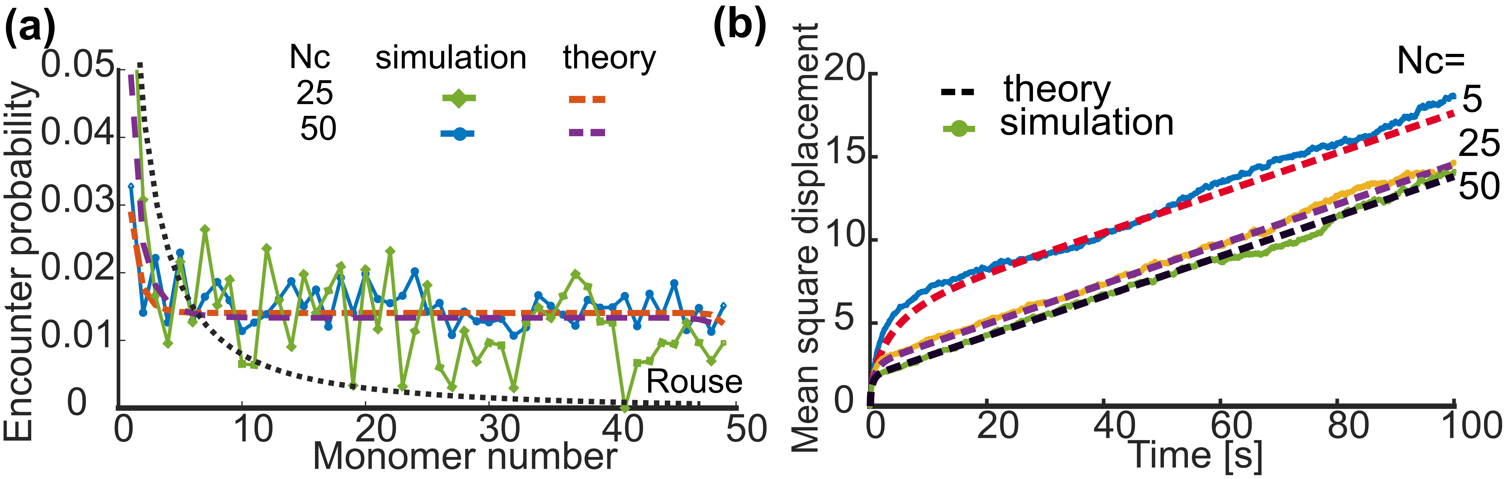
Figure 2: Dynamic properties of the RCL polymer (a) Simulation of encounter probability between monomers 1 and 2-50 of the RCL polymer. with $N=50$ monomers, where we added $N_{c}=25$ (green diamonds) and 50 (blue circles) connectors and compared with analytical formula Eq. 19 (dashed curves) for 500 realizations with $D=1,b=\sqrt{3},\epsilon=b/10,\Delta t=0.01s$. We show the encounter probability of the Rouse polymer ($N_{c}=0$ connectors, dotted black), which cannot account for long-range connectivity. (b) Simulation of the mean square displacement for a RCL polymer of $N=50$ monomer for $N_{c}=5$ (blue), 25 (yellow), and 50 (green) added connectors, shows excellent agreement with analytical formulas (Eq. 31, dashed).

Mean square radius of gyration (MSRG) of the RCL polymer. The MSRG $\langle R_{g}^{2}(\xi)\rangle$ characterizes the size of the RCL polymer and can be computed from the variance 25 as

$$\displaystyle\langle R_{G}^{2}(\xi)\rangle=\frac{1}{N^{2}}\sum_{m=1}^{N}\sum_{n=1}^{m}\sigma_{m,n}^{2}(\xi).$$ (27)

Using 25 and 27, with the notations $\zeta_{0}=\zeta_{0}(N,\xi),\quad\zeta_{1}=\zeta_{1}(N,\xi)$, we obtain

$$\langle R_{G}^{2}(\xi)\rangle=\frac{b^{2}}{N^{2}(1-\xi)(\zeta_{0}-\zeta_{1})}\Big{[}\frac{(1+2\zeta_{0})N(1+N)}{2\zeta_{0}}$$ (28)

$$+\frac{N(2(1+\zeta_{0})^{2}-\zeta_{0}^{3})}{1-\zeta_{0}^{2}}-\frac{\zeta_{0}^{3}(1-\frac{1}{\zeta_{0}^{2N}})}{(1-\zeta_{0}^{2})^{2}}+\frac{2(1+\zeta_{0})(1-\frac{1}{\zeta_{0}^{N}})}{(1-\zeta_{0})^{2}}\Big{]}.$$

When $N_{c}\ll\frac{N^{2}}{2}$, we obtain the asymptotic expansion

$$\langle R_{G}^{2}(\xi)\rangle\approx\frac{3b^{2}}{4}\sqrt{\frac{1}{N\xi}}.$$ (29)

In Fig. 1(d), we compare $\langle R_{G}^{2}(\xi)\rangle$ computed from Brownian simulations of $N=20,50$, and 100 monomers, with $N_{c}\in[5,50]$ added random connectors, with the asymptotic formula 28 and both agrees.
Mean Square Displacement (MSD) of a single monomer of the RCL polymer. Using the normal coordinates 9 in dimension $d$ the MSD of monomers in the RCL polymer is

$$\langle r_{m}^{2}(t)\rangle=\langle\left(\sum_{p=0}^{N-1}{\alpha_{p}^{m}u_{p}(t)}\right)^{2}\rangle=2dD_{cm}t+$$ (30)

$$\frac{2db^{2}}{N}\sum_{p=1}^{N-1}{\frac{\cos^{2}\left(\frac{p\pi(m-\frac{1}{2})}{N}\right)\left(1-\exp(-\frac{2D\chi_{p}(\xi)t}{b^{2}})\right)}{\chi_{p}(\xi)}},$$

where $D_{cm}=\frac{D}{N}$. Averaging over all monomers and approximating the sum in 30 by an integral for $N\gg 1$, we obtain

$$\langle\langle r_{m}^{2}(t)\rangle\rangle=2dD_{cm}t+\frac{db^{2}Erf[\sqrt{2dDN\xi t/b^{2}}]}{2\sqrt{N\xi(1-\xi)}},$$ (31)

where $Erf[t]$ is the error function. Equation 31 characterizes the MSD for intermediate time scale $\tau_{N-1}(\xi)\ll t\ll\tau_{1}(\xi)$. For short time scale $t\ll\tau_{N-1}(\xi)$, the MSD is given by

$$\langle\langle r_{m}^{2}(t)\rangle\rangle =\frac{db^{2}\int_{0}^{\sqrt{2dDN\xi t/b^{2}}}\exp(-g^{2})dg}{\sqrt{\pi N\xi(1-\xi)}}$$

$$\approx\frac{b\sqrt{2dDt}}{\sqrt{\pi(1-\xi)}}\left(1-\frac{\exp(-2dDN\xi t/b^{2})}{2}\right).$$

For $N\xi\gg 1$, the MSD behaves like

$$\langle\langle r_{m}^{2}(t)\rangle\rangle\propto\frac{db\sqrt{dDt}}{\sqrt{2\pi(1-\xi)}}.$$ (33)

We conclude that the homogeneous behavior of MSD for the RCL polymer model gives an anomalous exponent $\alpha=0.5$, similar to the Rouse model. Finally, for long time scales ($t\gg\tau_{1}(\xi)$), (slow diffusion of the polymer’s center of mass), the error function in 31 is almost constant and therefore

$$\langle\langle r_{m}(t)^{2}\rangle\rangle=2dD_{cm}t+\frac{db^{2}}{2\sqrt{N\xi(1-\xi)}}.$$ (34)

Mean First Encounter Time (MFET) $\langle\tau^{\epsilon}(\xi)\rangle$ between monomers of the RCL polymer. We compute here the mean time for two monomers of the RCL polymer to enter for the first time in a ball of radius $\epsilon>0$, at which they can possibly interact to form a chemical bond (Fig. 3(a)). The MFET for both the Rouse and beta Amitai and Holcman (2013) polymer were computed (see Amitai et al. (2012)) from the first eigenvalue $\lambda_{0}^{\epsilon}$ of the Fokker-Planck operator associated to the stochastic equation 13, so that

$$\langle\tau^{\epsilon}(\xi)\rangle\approx\frac{1}{D\lambda_{0}^{\epsilon}(\xi)}.$$ (35)

The first order approximation in $\epsilon$ is given by Amitai et al. (2012)

$$\lambda_{0}^{\epsilon}(\xi)=\frac{4\pi\epsilon\int_{C-P}e^{-\phi_{\xi}(U)}dU}{|\tilde{\Omega}(\xi)|}+O(\epsilon^{2}),$$ (36)

where $\phi_{\xi}(U)$ is the diagonalized potential 17, $|\tilde{\Omega}(\xi)|$ is the integral over the entire RCL configuration space

$$|\tilde{\Omega}(\xi)|=\int e^{-\phi_{\xi}(U)}dU=\left(\frac{(2\pi)^{N-1}}{\prod_{p=1}^{N-1}\kappa\chi_{p}(\xi)}\right)^{\frac{d}{2}}.$$ (37)

The integral over $C-P$ in 36 is computed over the space of closed RCL polymer ensemble, with fixed connector between monomers $m$ and $n$ and additional $N_{c}(\xi)$ random connectors. A direct computation gives

$$\int_{C-P}e^{-\phi_{\xi}(U)}dU=(2\pi)^{\frac{(N-2)d}{2}}\left(\frac{\kappa b^{2}\prod_{p=1}^{N-1}(\kappa\chi_{p}(\xi))^{-1}}{\sigma_{m,n}^{2}(\xi)}\right)^{\frac{d}{2}}.$$ (38)

Using relations 37 and 38 in 35, we obtain the MFET between any two monomers $m$ and $n$ of the RCL polymer for a given connectivity fraction $\xi$ in dimension $d=3$:

$$\langle\tau^{\epsilon}_{m,n}(\xi)\rangle=\frac{1}{4\pi D\epsilon}\left(\frac{2\pi\sigma_{m,n}^{2}(\xi)}{\kappa b^{2}}\right)^{\frac{3}{2}},$$ (39)

Using 26 into 39, we obtain the approximation

$$\langle\tau^{\epsilon}_{m,n}(\xi)\rangle\approx\frac{b^{2}\left(1-\exp(-|m-n|\sqrt{N\xi})\right)^{d/2}}{4\sqrt{N\xi}\pi D\epsilon(\kappa b^{2})^{d/2}}+\mathcal{O}(N\xi),$$

where $|m-n|\ll N$, and $\xi\ll 1$. The analytical formula 39 agrees with Brownian simulations of the MFET for RCL polymer (Eq. 3) with $N=20,50,$ and 100 monomers, and $N_{c}=25$ added random connectors (Fig. 3(b)).

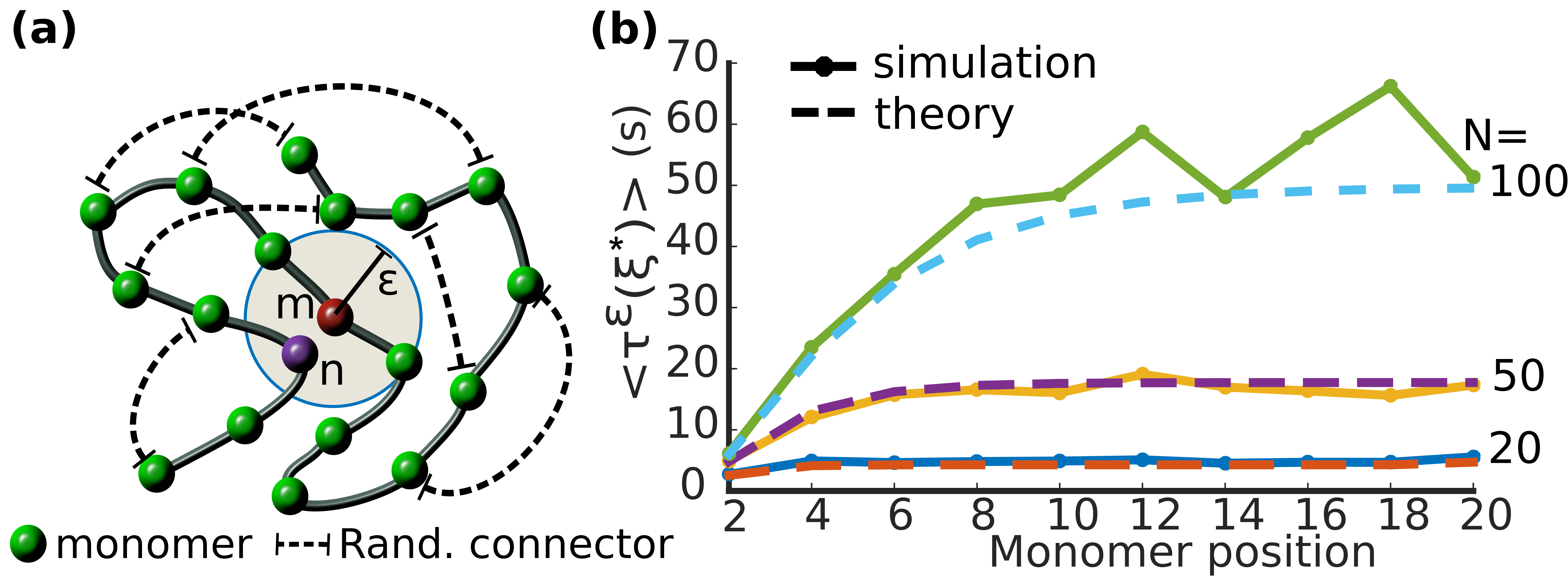
Figure 3: Transient properties of the RCL polymer (a) Two monomers $m$ (red) and $n$ (purple) of the RCL polymer meet when they enter a sphere of radius $\epsilon$. Random connectors (dashed arrows) are added to a linear Rouse backbone (b) Stochastic simulations (marked by a dot) MFET between monomer 1 and monomers 2-20 of RCL polymers with $N=20$ (blue), 50 (yellow) and 100 (green) monomers, with $N_{c}=25$ random connectors, are in good agreement with the analytical formula (Eq. 39, dashed). Parameters: $\epsilon=b/10,D=1,b=\sqrt{3},\Delta t=0.01s$, the RCL system is 3 (we used Eq. 39 with $\xi^{*}$, Eq. 18).

Applications of the RCL polymer model. We derived here several analytical formula for the steady-state variance, encounter probability, the radius of gyration, mean-square displacement and the mean first encounter time of the RCL polymer model. These formula can be used to extract parameters from chromatin conformation in CC experiments Dixon et al. (2012); Nora et al. (2012). In particular, using formula 19, it is possible to fit the empirical encounter probability obtained from experimental data to extract the connectivity fraction $\xi$. This parameter has a direct interpretation and represents the mean number of cross-links, that can be mediated by CTCF molecules present in a genomic region. The parameter $\xi$ depend on the coarse-grained scale (see Shukron and Holcman (2017)). The extracted parameter $\xi$ can then be used to estimate the radius of gyration (Eq. 28) of any region of interest. This radius characterizes the size of the genomic region, at least relative to other genomic segments, hence providing insightful information about the local organization of the chromatin in the cell nucleus.

To demonstrate out methodology, we coarse-grained the 5C data reported in Nora et al. (2012) of male neuronal progenitors NPC-E14 cells, replicate 1, TAD H, containing 679 kbp, at a scale of 3kbp, resulting in $N=226$ monomers. We fit the EP (Eq.19) to 5C data of each of the 226 monomers and obtain the average connectivity $\xi=0.0022$, corresponding $N_{c}=56$ added connectors. We use the persistence length of $b=0.05$ $\mu m$. Substituting $N=226,b=0.05,\xi=0.0022$ in Eq. 28, we compute the radius of gyration to be 43 nm for TAD H. Thus, the 679 kbp TAD H is compacted in a sphere of volume $3.4\times 10^{5}$ $nm^{3}$ (2 bp per $nm^{3}$).

The structural information extracted from the static CC maps using the RCL polymer model was recently used to interpret the dynamics of single particle trajectories (SPT) Gasser (2016); Lassadi et al. (2015); Amitai et al. (2017). By fitting the MSD (Eq. 31) to SPT data and by extracting the degree of connectivity $\xi$, we interpret the mean deviation of the loci dynamic from pure diffusion as the confined dynamics of the loci in a cross-links genomic environment Shukron and Holcman (2017); Weber et al. (2010a, b). We provided a direct formula to extract $\xi$, so that the simulations of Amitai et al. (2017) can now be bypassed. Finally, once the connectivity fraction is extracted, the mean first encounter time between any two monomers can be computed using formula 39. Encounter times are key for understanding processes, such as mammalian X chromosome inactivation Nora et al. (2012) or non-homologous-end joining after DNA double-strand break Amitai et al. (2017, 2012).

References

Nora et al. (2012)E. P. Nora, B. R. Lajoie,
E. G. Schulz, L. Giorgetti, I. Okamoto, N. Servant, T. Piolot, N. L. van Berkum, J. Meisig, J. Sedat, et al., Nature 485, 381 (2012).
Tark-Dame et al. (2014)M. Tark-Dame, H. Jerabek,
E. M. Manders, D. W. Heermann, and R. van Driel, PLoS Computational Biology 10, e1003877 (2014).
Dekker et al. (2002)J. Dekker, K. Rippe,
M. Dekker, and N. Kleckner, science 295, 1306 (2002).
Simonis et al. (2006)M. Simonis, P. Klous,
E. Splinter, Y. Moshkin, R. Willemsen, E. De Wit, B. Van Steensel, and W. De Laat, Nature genetics 38, 1348 (2006).
Lieberman-Aiden et al. (2009)E. Lieberman-Aiden, N. L. Van Berkum, L. Williams, M. Imakaev,
T. Ragoczy, A. Telling, I. Amit, B. R. Lajoie, P. J. Sabo, M. O. Dorschner, et al., science 326, 289 (2009).
Dixon et al. (2012)J. R. Dixon, S. Selvaraj,
F. Yue, A. Kim, Y. Li, Y. Shen, M. Hu, J. S. Liu, and B. Ren, Nature 485, 376 (2012).
Doi and Edwards (1986)M. Doi and S. Edwards, The Theory of Polymer Dynamics
Clarendon (Oxford, 1986).
Shukron and Holcman (2017)O. Shukron and D. Holcman, PLOS
Computational Biology 13, e1005469 (2017).