Beamforming Optimization for Full-Duplex Wireless-powered MIMO Systems

Abstract

We propose techniques for optimizing transmit beamforming in a full-duplex multiple-input-multiple-output (MIMO) wireless-powered communication system, which consists of two phases. In the first phase, the wireless-powered mobile station (MS) harvests energy using signals from the base station (BS), whereas in the second phase, both MS and BS communicate to each other in a full-duplex mode. When complete instantaneous channel state information (CSI) is available, the BS beamformer and the time-splitting (TS) parameter of energy harvesting are jointly optimized in order to obtain the BS-MS rate region. The joint optimization problem is non-convex, however, a computationally efficient optimum technique, based upon semidefinite relaxation and line-search, is proposed to solve the problem. A sub-optimum zero-forcing approach is also proposed, in which a closed-form solution of TS parameter is obtained. When only second-order statistics of transmit CSI is available, we propose to maximize the ergodic information rate at the MS, while maintaining the outage probability at the BS below a certain threshold. An upper bound for the outage probability is also derived and an approximate convex optimization framework is proposed for efficiently solving the underlying non-convex problem. Simulations demonstrate the advantages of the proposed methods over the sub-optimum and half-duplex ones.

I Introduction

Proliferation of communication devices, systems and networks has considerably increased the demand for wireless spectrum, driving the interest to design systems with higher spectral efficiency. Most contemporary bi-directional wireless systems have been developed for half-duplex (HD) operation (i.e., either transmit or receive, but not both simultaneously). As an effective method of improving the spectral efficiency of contemporary HD systems, full-duplex (FD) communications have emerged as a promising solution [1, 2]. Although the concept of FD is not new and has been in use since 1940s, so far it has been considered as impossible to realize due to the loopback interference (LI) that couples the device output to the input [3, 4]. However, FD is now becoming feasible, thanks to promising analog/digital and spatial domain LI cancellation techniques that can achieve high transmit-receive isolation [5, 6, 7, 8]. As a result, experimental demonstration of the feasibility of FD has already been carried out by several research laboratories.

FD communications can be implemented for three basic topologies, namely, (a) relay topology (b) bidirectional topology and (c) base station (BS) topology [1]. To this end, bidirectional FD systems have been investigated in some existing works in the literature [10, 12, 9, 11]. These include papers that have focused on information-communication theoretic performance metrics, such as the achievable sum rate and symbol error probability. In [10], achievable upper and lower sum-rate bounds of multiple antenna bidirectional communication, that use pilot-aided channel estimates for transmit/receive beamforming and interference cancellation, were derived. The beamforming performance of bidirectional multiple-input multiple-output (MIMO) transmission with spatial LI mitigation was investigated in [9]. Furthermore, capacity of a bidirectional MIMO system with spatial correlation was presented in [11]. Finally, the maximization of the asymptotic ergodic mutual information for a MIMO bi-directional communication system, with imperfect channel state information (CSI), was the focus of the work in [12].

In addition to the spectral efficiency, energy efficiency has gained wide research attention for the design of wireless networks. For example, energy constraints impose an upper limit on the transmit power and the associated signal processing in wireless devices. To this end, a new paradigm that can power communication devices via energy harvesting techniques has emerged [13, 14]. Among different energy harvesting sources such as ambient heat, wind, solar, vibration, etc., wireless power transfer (WPT) using dedicated radio frequency sources is regarded as a promising solution, since it can be controlled to achieve optimum performance. Therefore, WPT can be used to remotely power a variety of applications such as wireless sensor networks, body area networks, wireless charging facilities and future cellular networks [13, 14, 15]. Moreover, since wireless signals can transport both information and energy, by introducing the new notion of “simultaneous wireless information and power transfer” (SWIPT), the rate-energy region of a wireless-powered MIMO broadcast network with an external energy harvester was characterized in [16]. In [17], throughput performance of a wireless-powered network in which a multi-antenna hybrid access point (H-AP) beamforms energy to a single antenna user in order to assist uplink information transfer was presented. Motivated by the advantages of FD and WPT, some recent works have also investigated the performance of wireless-powered bidirectional communications [18, 19, 21, 20].

In wireless-powered FD networks, the deployment of multiple antennas can be considered as a practical solution, since the strategy is useful to harvest higher amount of energy [22] as well as to deploy spatial beamforming techniques to suppress LI [5]. In [18], considering a FD H-AP that broadcasts wireless energy to a set of downlink users while receiving information from a set of uplink users, a solution to an optimal resource allocation problem was presented. In [19], hardware implementation of a wireless system, that transmits data and power in the same frequency, was presented. In [20], performance of a wireless-powered FD communication network, which consists of a dual-antenna FD H-AP and a single dual-antenna FD user, was investigated. Specifically, assuming different roles for the two antennas (downlink WPT or uplink wireless information transfer), closed-form expressions for the system’s outage probability and the ergodic capacity were derived. More recently, in [21], a weighted sum transmit power optimization problem for a bidirectional FD system with WPT was formulated and solved. However, it assumes perfect LI cancellation at terminals which is impossible in practice [4].

Inspired by wireless-powered FD communications, in this paper, we consider bidirectional communication between an $N$-antenna BS and a mobile station (MS) with two antennas. According to “harvest-then-transmit” protocol [23], the BS first transmits energy to the MS, which is used by the MS for the subsequent uplink transmission. At the end of the energy transfer phase, both BS and MS simultaneously transfer information in the uplink and downlink, thanks due to the FD operation. Specifically for this setup, we propose methods for jointly optimizing the beamformer at the BS and the time-splitting (TS) parameter that divides a given time-slot into energy harvesting and data transmission phases. Both full and partial CSI cases are considered. In the former case, where the instantaneous channel is known, the optimized boundary of the BS-MS rate region is obtained, which describes the trade-off between BS and MS information rate. To this end, a computationally efficient optimum method, based upon semidefinite relaxation (SDR) and line-search, is proposed and its performance is compared with a sub-optimum method that uses the zero-forcing (ZF) criterion for designing the beamformer.

In the partial CSI case, the BS and MS know only the second-order statistics, such as channel covariance matrices, of their transmit CSI. It is also worth mentioning that the BS rate turns to be much smaller than the MS rate, since the MS transmits with the harvested energy which, in general, is much smaller than the transmit power of the BS. Moreover, the maximum possible value of the BS rate cannot be achieved in the partial CSI case. Due to these reasons, it is important to ensure that the BS is not in outage rather than maximize the BS-rate which is already constrained by the MS’s transmit power. Hence, we propose to maximize the ergodic information rate at the MS, while ensuring that the outage probability at the BS remains below a certain threshold value. This optimization problem is non-convex and non-tractable. As such, we derive an upper bound of the BS outage probability, and formulate an optimization problem so that the gap between the derived upper bound and the exact outage probability remains minimum. In particular, using the upper bound of the outage probability, we maximize the ergodic information rate at the MS. We utilize the monotonicity property of the derived exact ergodic information rate and formulate an SDR optimization problem, that is efficiently solved with a convex optimization toolbox.

The main contributions of this paper are summarized as follows:

• In the case of full CSI, the joint optimization problem of transmit beamforming and TS parameter is efficiently solved as an SDR problem. The optimality of the relaxation is confirmed with a proof that the optimum solution of the relaxed problem is rank-one.

• We show that the MS-rate is a monotonically decreasing function of the TS parameter, and this property is utilized to efficiently solve the SDR-based joint optimization. A closed-form expression of the TS parameter is derived in the ZF-based sub-optimum design.

• Closed-form expressions for the ergodic MS-rate and BS outage probability are derived. For a given TS parameter, we show that the ergodic MS-rate is a monotonically increasing function of the beamformer gain towards the MS. We, then, utilize this property for solving the problem of maximizing the MS ergodic rate, while satisfying the outage probability constraint at the BS.

• Since the optimization problem remains non-tractable with the original outage probability, we derive its upper bound and approximate the original optimization problem with the SDR problem. The proposed optimization tries to minimize the gap between the exact outage probability and its upper bound.

The rest of the paper is organized as follows. The system model and problem formulation are presented in Section II. The optimization problems for full and partial CSI cases are solved in sections III and IV, respectively. In Section V, numerical results are provided, whereas in Section VI, conclusions are drawn.

Notation: Upper (lower) bold face letters will be used for matrices (vectors); $(\cdot)^{T}$, $(\cdot)^{H}$, ${\rm E}\left\{\cdot\right\}$, ${\bf I}$ and $||{\cdot}||$ denote transpose, Hermitian transpose, expectation w.r.t. a random variable $x$, identity matrix, and Frobenius norm (Euclidean norm for a vector), respectively. ${\rm tr}(\cdot)$, ${\mathcal{C}}^{M\times M}$, and ${\bf A}\succeq 0$ denote the matrix trace operator, space of $M\times M$ matrices with complex entries, and positive semidefiniteness of ${\bf A}$, respectively.

II System Model and Problem Formulation

We consider bidirectional FD communications between an $N$-antenna BS and a MS as shown in Fig. 1. Specifically, the BS has $N_{t}$ transmit antennas and $N_{r}\triangleq N-N_{t}$ receive antennas. Notice that, $N_{t}$, together with the chosen transmit/receive antennas could be optimized, but we keep them fixed. Although joint antenna selection and beamformer optimization is an interesting future work, it requires a multi-stage optimization approach and, thus, is is not considered in this work. The MS is an energy constrained device and harvests energy from the signals transmitted by the BS. The MS, then, utilizes the harvested energy for its uplink transmission. Since the MS is energy constrained and depends on the harvested energy (which assumes typically small values), as in [21] we assume that the MS is equipped with two antennas (one antenna of the MS is used for transmission, whereas the other is used for reception). This assumption is further motivated by the fact that the space constraint prevents mounting more antennas at the MS. Moreover, since the BS is equipped with multiple antennas in our system, for sufficient amounts of energy harvesting, beamforming can be effectively used [16].

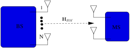
(a) EH phase of duration $\alpha T$.

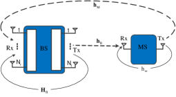
(b) FD communication phase of duration $(1-\alpha)T$.

Figure 1: Two phases of wireless-powered communication system.

Without loss of generality, assuming a block time of $T=1$, communication between the BS and MS takes place in two phases with duration $\alpha$ and $(1-\alpha)$, respectively. In phase I, the BS employs all of its antennas to transmit energy, whereas the MS employs both of its antennas for reception. The signal received by the MS during energy harvesting phase is given by ${\bf y}_{E}={\bf H}_{BM}{\bf w}_{E}s_{E}+{\bf n}_{E}$, where ${\bf H}_{BM}\in{\mathcal{C}}^{2\times N}$ is the channel between the BS and the MS, ${\bf w}_{E}\in{\mathcal{C}}^{N\times 1}$ is the energy beamformer, $s_{E}$ is the signal transmitted by the BS, and ${\bf n}_{E}$ is the additive white Gaussian noise (AWGN) at the MS. We assume that the harvested energy due to the noise (including both the antenna noise and the rectifier noise) is small and thus ignored [25]. Thus, assuming that ${\rm E}\{|s_{E}|^{2}\}=1$ during the period of $\alpha$, the harvested energy can be expressed as $E=\eta\alpha||{\bf H}_{BM}{\bf w}_{E}||^{2}=\eta\alpha{\rm tr}\left({\bf w}^{H}_{E}{\bf H}^{H}_{BM}{\bf H}_{BM}{\bf w}_{E}\right)$, where $\eta$ is the conversion efficiency of the rectifier circuit at the MS. Considering that $||{\bf w}_{E}||^{2}=P$, where $P$ is the total transmit power of the BS during energy harvesting phase, it is clear that the optimum ${\bf w}_{E}$ is given by ${\bf w}_{E}=\sqrt{P}{\bf v}_{\rm max}$, where ${\bf v}_{\rm max}$ is the eigenvector corresponding to the largest eigenvalue of the matrix ${\bf H}^{H}_{BM}{\bf H}_{BM}$. This means, the harvested energy is given by

$$E=P\alpha{\bar{\lambda}}{\left({\bf H}_{BM}{\bf H}_{BM}^{H}\right)},$$ (1)

where the channel between the BS and the MS is denoted as ${\bf H}_{BM}$ and ${\bar{\lambda}}(\cdot)$ returns the maximum eigenvalue of a matrix. As such, the BS requires transmit CSI which is obtained through reverse-link training via channel reciprocity[26] approach. More specifically, assuming that the BS-MS and MS-BS channels are reciprocal, the MS first sends training and the BS then estimates the channel and performs optimum energy beamforming. Although it requires CSI at the BS, the harvested energy due to beamforming gain can be much larger than the energy consumed for sending training signals [26]. On the other hand, we will relax the full CSI requirement by considering partial CSI case and solving the corresponding optimization problem in Section IV. Thus, the reported results of the full CSI case serve as useful theoretical bounds for practical design.

Note that, in (1) the energy that can be harvested from noise is omitted since for all practical purposes it is negligible. ${\bf H}_{BM}$ is expressed as ${\bf H}_{BM}=\sqrt{\frac{1}{d^{\tau}}}{\bar{\bf H}}_{BM}$, where $d$ is the distance between the BS and MS, $\tau$ is the path loss exponent, and each element of ${\bar{\bf H}}_{BM}$ has zero-mean and unit-variance. In phase II, since both terminals operate in the FD mode, the BS and MS simultaneously communicate with each other. The transmit power of MS can be written as

$$p_{m}=\frac{\alpha\eta P{\bar{\lambda}}{\left({\bf H}_{BM}{\bf H}_{BM}^{H}\right)}}{(1-\alpha)},$$ (2)

where $\eta$ is the conversion efficiency of wireless energy transfer. Let the $1\times N_{t}$ $BS\rightarrow MS$ channel be ${\bf h}_{B}^{H}=\sqrt{\frac{1}{d^{\tau}}}{\bar{\bf h}}_{B}^{H}$ and the $(N-N_{t})\times 1$ $MS\rightarrow BS$ channel be ${\bf h}_{M}=\sqrt{\frac{1}{d^{\tau}}}{\bar{\bf h}}_{M}$, where all elements of ${\bar{\bf h}}_{B}$ and ${\bar{\bf h}}_{M}$ have zero-mean and unit variance. The residual LI channels are ${\bf H}_{B}\in\mathbb{C}^{(N-N_{t})\times N_{t}}$ and $h_{m}$ at the BS and MS, respectively. In order to reduce the deleterious effects of LI on system performance, we assume that an analog/digital cancellation scheme can be employed at the BS and MS, respectively and as such the residual channels are modeled as feedback fading channels [4, 5]. Since such a cancellation scheme can be characterized by a specific residual power, each element of ${\bf H}_{B}$, and $h_{m}$ can be modeled as zero-mean circularly symmetric complex Gaussian (ZMCSCG) random variables of variances $\sigma^{2}_{h_{b}}$ and $\sigma^{2}_{h_{m}}$, respectively. Modeling of the residual LI channel in such a way is now common and a standard assumption in the FD literature since the dominant line-of-sight component in LI can be removed effectively when a cancellation method is implemented [6]. It is also important to emphasize that perfect cancellation of LI is not possible due to imperfect estimation of LI channel, inevitable transceiver chain impairments [5], [24], and inherent processing delay. Therefore, ${\bf H}_{B}$ and $h_{m}$ can assume relatively large values and their effects can be minimized with spatial suppression techniques [25].

II-A Signal Model

The received signals at the BS and MS, are, respectively

$${\bf y}_{B}=\sqrt{p_{m}}{\bf h}_{M}s_{M}+{\bf H}_{B}{\bf w}_{B}s_{B}+{\bf n}_{B},$$

$$y_{M}={\bf h}_{B}^{H}{\bf w}_{B}s_{B}+\sqrt{p_{m}}h_{m}s_{M}+n_{M},$$ (3)

where ${\bf y}_{B}\in{\mathcal{C}}^{(N-N_{t})\times 1}$, $s_{M}$ and $s_{B}$ are the information symbols transmitted by the MS and BS, respectively, ${\bf w}_{B}\in{\mathcal{C}}^{N_{t}\times 1}$ is the beamformer at the BS, ${\bf n}_{B}\in{\mathcal{C}}^{(N-N_{t})\times 1}$ is the additive White Gaussian noise (AWGN) vector at the receive antenna elements of the BS, and $n_{M}\in{\mathcal{C}}$ is the AWGN at the receive antenna of the MS. Furthermore, it is assumed that ${\rm E}\left\{s_{B}\right\}={\rm E}\left\{s_{M}\right\}=0$, ${\rm E}\left\{|s_{B}|^{2}\right\}={\rm E}\left\{|s_{M}|^{2}\right\}=1$, ${\rm E}\left\{{\bf n}_{B}\right\}={\bf 0}$, ${\rm E}\left\{n_{M}\right\}=0$, ${\rm E}\left\{{\bf n}_{B}{\bf n}_{B}^{H}\right\}=\sigma_{b}^{2}{\bf I}_{(N-N_{t})}$, ${\rm E}\left\{|n_{M}|^{2}\right\}=\sigma_{m}^{2}$, and signals and noise are statistically independent. We also consider that $||{\bf w}_{B}||^{2}=P$, which means that the BS transmits with the same power, $P$, during both energy harvesting and communication phases. It is worthwhile to note that the BS can transmit different powers in two phases and the system performance can be further improved by optimizing these powers. However, this leads to a new optimization problem which is beyond the scope of the current work.

The BS applies a beamformer ${\bf r}_{B}\in{\mathcal{C}}^{(N-N_{t})\times 1}$ to the received signal ${\bf y}_{B}$. Without loss of generality, it is assumed that $||{\bf r}_{B}||=1$. The output after beamforming is given by

$$y_{B}={\bf r}^{H}_{B}{\bf y}_{B}={\bf r}^{H}_{B}\left(\sqrt{p_{m}}{\bf h}_{M}s_{M}+{\bf H}_{B}{\bf w}_{B}s_{B}+{\bf n}_{B}\right).$$ (4)

The signal-to-interference-and-noise ratio (SINR) at the BS and MS are then given by

$$SINR_{B} = \frac{p_{m}|{\bf r}_{B}^{H}{\bf h}_{M}|^{2}}{\sigma_{b}^{2}+|{\bf r}_{B}^{H}{\bf H}_{B}{\bf w}_{B}|^{2}},$$ (5)

and

$$SINR_{M} = \frac{|{\bf h}_{B}^{H}{\bf w}_{B}|^{2}}{\sigma_{m}^{2}+p_{m}|h_{m}|^{2}},$$ (6)

respectively. For a given ${\bf w}_{B}$, the optimum ${\bf r}_{B}$ is the one that maximizes $SINR_{B}$ and, thus, is obtained by solving

$$\max\limits_{||{\bf r}_{B}||=1}\frac{{\bf r}_{B}^{H}{\bf h}_{M}{\bf h}^{H}_{M}{\bf r}_{B}}{{\bf r}_{B}^{H}\left(\sigma_{b}^{2}{\bf I}+{\bf H}_{B}{\bf w}_{B}{\bf w}_{B}^{H}{\bf H}_{B}^{H}\right){\bf r}_{B}},$$ (7)

which is in generalized Rayleigh quotient form [27]. It is well known that the maximum value in (7) is obtained when

$${\bf r}_{B}=\frac{\left(\sigma_{b}^{2}{\bf I}+{\bf H}_{B}{\bf w}_{B}{\bf w}_{B}^{H}{\bf H}_{B}^{H}\right)^{-1}{\bf h}_{M}}{||\left(\sigma_{b}^{2}{\bf I}+{\bf H}_{B}{\bf w}_{B}{\bf w}_{B}^{H}{\bf H}_{B}^{H}\right)^{-1}{\bf h}_{M}||}.$$ (8)

Substituting the optimum ${\bf r}_{B}$ into $SINR_{B}$, it is clear that

$$SINR_{B}=p_{m}{\bf h}_{M}^{H}(\sigma_{b}^{2}{\bf I}+{\bf H}_{B}{\bf w}_{B}{\bf w}_{B}^{H}{\bf H}_{B}^{H})^{-1}{\bf h}_{M}.$$ (9)

Consequently, the BS achievable rate is given by

$$r_{B}=(1-\alpha)\log_{2}\left(1+p_{m}{\bf h}_{M}^{H}(\sigma_{b}^{2}{\bf I}+{\bf H}_{B}{\bf w}_{B}{\bf w}_{B}^{H}{\bf H}_{B}^{H})^{-1}{\bf h}_{M}\right),$$

which with the help of Sherman-Morrison formula [28] can also be expressed as

$$r_{B} = (1-\alpha)\log_{2}\left(1+\frac{p_{m}}{\sigma_{b}^{2}}\left(\|{\bf h}_{M}\|^{2}-\frac{|{\bf h}_{M}^{H}{\bf H}_{B}{\bf w}_{B}|^{2}}{\sigma_{b}^{2}+\|{\bf H}_{B}{\bf w}_{B}\|^{2}}\right)\right).$$

On the other hand, the achievable rate at the MS can be written as

$$r_{M} = (1-\alpha)\log_{2}\left(1+\frac{|{\bf h}_{B}^{H}{\bf w}_{B}|^{2}}{\sigma_{m}^{2}+p_{m}|h_{m}|^{2}}\right).$$ (10)

II-B Problem Formulation

Our objective is to characterize the bidirectional communications with the MS-BS rate region. It can be obtained by maximizing the MS rate while ensuring that the BS-rate is equal to a certain value, $R_{B}$. By solving this optimization problem for all $R_{B}$, where $R_{B}\in[0,R_{B}^{\rm max}]$ and $R_{B}^{\rm max}$ is the maximum value of BS rate, we obtain the MS-BS rate region. Note that $R_{B}^{\rm max}$ is obtained by solving $R_{B}^{\rm max}=\max\limits_{||{\bf w}_{B}||=1}r_{B}$. The closed-form expression of $R_{B}^{\rm max}$ is derived in Appendix A. As such, the optimization problem for a given $R_{B}$ is expressed as

$$\max_{\{{\bf w}_{B},\alpha\}} ~{}(1-\alpha)\log_{2}\left(1+\frac{|{\bf h}_{B}^{H}{\bf w}_{B}|^{2}}{\sigma_{m}^{2}+p_{m}|h_{m}|^{2}}\right)$$

s.t. $$(1-\alpha)\log_{2}\biggl{(}1+\frac{p_{m}}{\sigma_{b}^{2}}\|{\bf h}_{M}\|^{2}-\biggr{.}$$ (11)

$$\hskip 42.67912pt\biggl{.}\frac{\frac{p_{m}}{\sigma_{b}^{2}}|{\bf h}_{M}^{H}{\bf H}_{B}{\bf w}_{B}|^{2}}{\sigma_{b}^{2}+\|{\bf H}_{B}{\bf w}_{B}\|^{2}}\biggr{)}=R_{B},$$

$$||{\bf w}_{B}||^{2}\leq P,~{}~{}0<\alpha<1,$$

$$p_{m}=\frac{\alpha\eta P{\bar{\lambda}}{\left({\bf H}_{BM}{\bf H}_{BM}^{H}\right)}}{(1-\alpha)}.$$

The optimization problem in (II-B) is a complicated non-convex problem, w.r.t. ${\bf w}_{B}$ and $\alpha$. However, it can be efficiently solved by finding the optimum ${\bf w}_{B}$ for a given $\alpha$ and vice-versa. Since $\alpha$ is a scalar, the optimum solution can be ascertained by using one-dimensional search, w.r.t. $\alpha$.

III Joint Optimization with Perfect CSI

In this section, we propose the optimum and sub-optimum methods for solving the joint optimization of beamformer and the TS parameter in (II-B), when perfect CSI is available. In practice, CSI is subject to different types of errors (e.g., channel estimation, feedback, delay and quantization errors) and, hence, the joint optimization with the assumption of perfect CSI enables us to obtain the outer boundary of the BS-MS rate region. Such a boundary provides an upper bound performance that can be achieved by a system that is subject to erroneous CSI.

III-A Optimum Method

In this method, the jointly optimal ${\bf w}_{B}$ and $\alpha$ are determined by obtaining the optimum ${\bf w}_{B}$ for each $\alpha$, and then choosing those ${\bf w}_{B}$ and $\alpha$ that maximize the objective function in (II-B). For this purpose, a grid-search over $\alpha$ is required, which is just one-dimensional (or linear). Exploiting the structure of the problem (II-B), we show that the required grid search can be limited to a small region of $\alpha$, and hence, the computational cost for solving the joint optimization is minimized.

III-A1 Optimization of ${\bf w}_{B}$

We first consider a problem to optimize ${\bf w}_{B}$ for a given $\alpha$. In this case, the optimization problem in (II-B) is expressed as

$$\max_{{\bf w}_{B}}~{} ~{}(1-\alpha)\log_{2}\left(1+\frac{|{\bf h}_{B}^{H}{\bf w}_{B}|^{2}}{\sigma_{m}^{2}+p_{m}|h_{m}|^{2}}\right)$$

s.t. $$(1-\alpha)\log_{2}\biggl{(}1+\frac{p_{m}}{\sigma_{b}^{2}}\|{\bf h}_{M}\|^{2}-\biggr{.}$$ (12)

$$\hskip 42.67912pt\biggl{.}\frac{\frac{p_{m}}{\sigma_{b}^{2}}|{\bf h}_{M}^{H}{\bf H}_{B}{\bf w}_{B}|^{2}}{\sigma_{b}^{2}+\|{\bf H}_{B}{\bf w}_{B}\|^{2}}\biggr{)}=R_{B},$$

$$||{\bf w}_{B}||^{2}\leq P.$$

Since $\log(1+x)$ is a monotonically increasing function of $x$ and the denominator of $x\triangleq\frac{|{\bf h}_{B}^{H}{\bf w}_{B}|^{2}}{\sigma_{m}^{2}+p_{m}|h_{m}|^{2}}$ is independent of ${\bf w}_{B}$, (III-A1) can be solved via

$$\max_{{\bf w}_{B}}~{} |{\bf h}_{B}^{H}{\bf w}_{B}|^{2}$$

s.t. $$\frac{|{\bf h}_{M}^{H}{\bf H}_{B}{\bf w}_{B}|^{2}}{\sigma_{b}^{2}+\|{\bf H}_{B}{\bf w}_{B}\|^{2}}=\Gamma_{B},$$

$$\|{\bf w}_{B}\|^{2}\leq P$$

where $\Gamma_{B}\triangleq||{\bf h}_{M}||^{2}-\frac{\sigma_{b}^{2}}{p_{m}}\left[2^{\frac{R_{B}}{1-\alpha}}-1\right]$. It is clear that the objective function in (III-A1) is maximized when $||{\bf w}_{B}||^{2}=P$. This optimization problem is non-convex because it is the maximization of a quadratic function with a quadratic equality constraint. Moreover, to the best of our knowledge, (III-A1) does not admit a closed-form solution. However, it can be efficiently and optimally solved using semi-definite programming. For this purpose, we define ${\bf V}_{B}\triangleq{\bf w}_{B}{\bf w}_{B}^{H}$ and relax the rank-one constraint, ${\rm rank}({\bf V}_{B})=1$. The relaxed form of (III-A1) is given by

$$\max_{{\bf V}_{B}}~{} f(\alpha)={\rm tr}({\bf V}_{B}{\bf h}_{B}{\bf h}_{B}^{H})$$

s.t. $${\rm tr}({\bf V}_{B}{\bf H}_{B}^{H}{\bf h}_{M}{\bf h}_{M}^{H}{\bf H}_{B})=\Gamma_{B}\left(\sigma_{b}^{2}+{\rm tr}({\bf V}_{B}{\bf H}_{B}^{H}{\bf H}_{B})\right),$$ (14)

$${\rm tr}({\bf V}_{B})=P,~{}{\bf V}_{B}\succeq 0.$$

The optimization problem in (III-A1) is a standard SDR problem [29]. In the following, we show that its optimum solution is rank-one.

Proposition 1.

The rank-one optimum solution is guaranteed in (III-A1).

Proof.

The proof is based on Karush-Kuhn-Tucker (KKT) conditions and given in Appendix B. ∎

Let ${\bf V}_{B}^{*}$ be the optimum solution of (III-A1). Since ${\bf V}_{B}^{*}$ is a rank-one matrix, the optimum solution ${\bf w}_{B}^{*}$ is obtained as ${\bf w}_{B}^{*}=\sqrt{P}{\tilde{\bf u}}{\tilde{\bf u}}^{H}$, where ${\tilde{\bf u}}$ is the eigenvector corresponding to the non-zero eigenvalue of ${\bf V}_{B}^{*}$ .

III-A2 Optimization of ${\bf w}_{B}$ and $\alpha$

In order to jointly optimize ${\bf w}_{B}$ and $\alpha$, we solve the SDR problem in (III-A1) by using one-dimensional (or line search) search over $\alpha$. This line search can be confined to a small region of $\alpha$, and therefore, the number of required SDR optimizations can be significantly minimized. To illustrate this, let the objective function in (III-A1), for a given ${\bf w}_{B}^{*}$, be defined as

$$f(\alpha)=(1-\alpha)\log_{2}\left(1+\frac{{\tilde{\beta}}}{c+\frac{\alpha b}{1-\alpha}}\right)$$ (15)

where

$${\tilde{\beta}}=\frac{|{\bf h}_{B}^{H}{\bf w}_{B}^{*}|^{2}}{|h_{m}|^{2}},c=\frac{\sigma_{m}^{2}}{|h_{m}|^{2}},b=\eta P{\bar{\lambda}}\left({\bf H}_{BM}{\bf H}_{BM}^{H}\right).$$ (16)

The derivative of $f(\alpha)$ w.r.t. $\alpha$ can be written as

$$\frac{df(\alpha)}{d\alpha}=-\log_{2}(g(\alpha))-\frac{b{\tilde{\beta}}g(\alpha)^{-1}}{(1-\alpha)\log(2)}\left(c+\frac{\alpha b}{1-\alpha}\right)^{-2}$$ (17)

where $g(\alpha)=1+\frac{{\tilde{\beta}}}{c+\frac{\alpha b}{1-\alpha}}\geq 0,\forall\alpha\in[0,1]$. It is clear from (17) that $\frac{df(\alpha)}{d\alpha}<0$ for all $\alpha$, i.e., $f(\alpha)$ is a monotonically decreasing function of $\alpha$. This means that maximum value of the objective function in (15) is achieved when $\alpha$ is minimum, provided that the equality constraint in (III-A1) is fulfilled. However, as $\alpha\rightarrow 0$, $\Gamma_{B}\rightarrow-\infty$, i.e., the chance that the SDR optimization problem (III-A1) is infeasible increases. Consequently, the optimum $\alpha$ is the minimum one for which (III-A1) is feasible. The output ${\bf V}_{B}$ of such feasible SDR provides the optimum ${\bf w}_{B}$. In a nutshell, the steps of the proposed algorithm (Algorithm 1) for the joint optimization problem can be summarized as follows:

• 1) Define a fine grid of $\alpha$ in steps of $\partial\alpha$. Start with $\alpha=0$.

• 2) Solve (III-A1) with the increment of $\partial\alpha$.

• 3) If feasible, stop and output $\alpha$ and ${\bf V}_{B}$.

• 4) If not, go to step (2).

Since this algorithm terminates as soon as (III-A1) is feasible, the search region of $\alpha$ is usually limited to a range of its small values. We use CVX toolbox [29] to solve the SDR problem (III-A1). For a given solution accuracy of $\epsilon>0$, the worst-case complexity of this optimization problem is given by ${\mathcal{O}}\left(N_{t}^{4.5}\log\left(\frac{1}{\epsilon}\right)\right)$ [30]. While executing Algorithm 1, the SDR problem is solved for that particular $\alpha$ for which the problem is feasible. Note that, by considering that $\Gamma_{B}$ should be positive and $||{\bf w}_{B}||^{2}\leq P$, necessary conditions for the feasibility [31] of (III-A1) can be checked before calling the CVX routine. Therefore, the worst-case computational complexity of executing Algorithm 1 is only ${\mathcal{O}}\left(N_{t}^{4.5}\log\left(\frac{1}{\epsilon}\right)\right)$.

III-B Suboptimal Method

As a suboptimal method of optimizing ${\bf w}_{B}$ and $\alpha$, we consider the ZF approach [32]. This requires that

$${\bf w}_{B}^{H}{\bf H}_{B}^{H}{\bf h}_{M}=0.$$ (18)

III-B1 Optimization of ${\bf w}_{B}$

Substituting (18) into (II-B), the resulting optimization problem is expressed as

$$\max_{\{{\bf w}_{B},\alpha\}}~{} (1-\alpha)\log_{2}\left(1+\frac{|{\bf h}_{B}^{H}{\bf w}_{B}|^{2}}{\sigma_{m}^{2}+p_{m}|h_{m}|^{2}}\right)$$

s.t. $$(1-\alpha)\log_{2}\left(1+\frac{p_{m}}{\sigma_{b}^{2}}\|{\bf h}_{M}\|^{2}\right)=R_{B},$$

$$p_{m}=\frac{\alpha\eta P{\bar{\lambda}}{\left({\bf H}_{BM}{\bf H}_{BM}^{H}\right)}}{1-\alpha}$$

$$\|{\bf w}_{B}\|^{2}\leq P,~{}~{}0\leq\alpha\leq 1,$$

$${\bf w}_{B}^{H}{\bf H}_{B}^{H}{\bf h}_{M}=0.$$

For a given $\alpha$, the optimization of ${\bf w}_{B}$ becomes

$$\max_{{\bf w}_{B}} |{\bf h}_{B}^{H}{\bf w}_{B}|^{2}$$

s.t. $$\|{\bf w}_{B}\|^{2}\leq P$$

$${\bf w}_{B}^{H}{\bf H}_{B}^{H}{\bf h}_{M}=0.$$

Using the standard Lagrangian multiplier method and after some manipulations, a closed-form solution of ${\bf w}_{B}$ is obtained as

$${\bf w}_{B}=\sqrt{P}\frac{{\bf B}{\bf h}_{B}}{\|{\bf B}{\bf h}_{B}\|},{\bf B}={\bf I}-\frac{{\bf H}_{B}^{H}{\bf h}_{M}{\bf h}_{M}^{H}{\bf H}_{B}}{\|{\bf H}_{B}^{H}{\bf h}_{M}\|^{2}}$$ (21)

where ${\bf w}_{B}$ does not depend on $\alpha$ and ${\bf B}$ is a projection matrix, i.e., ${\bf B}^{H}{\bf B}={\bf B}$. Consequently, the corresponding objective function in (III-B1) is

$$|{\bf h}_{B}^{H}{\bf w}_{B}|^{2}=P\frac{|{\bf h}_{B}^{H}{\bf B}{\bf h}_{B}|^{2}}{\|{\bf B}{\bf h}_{B}\|^{2}}=P{\bf h}_{B}^{H}{\bf B}{\bf h}_{B}.$$ (22)

III-B2 Optimization of $\alpha$

Denote the suboptimal beamformer solution of (21) by ${\bar{\bf w}}_{B}^{*}$. The remaining optimization problem is expressed as

$$\max_{0\leq\alpha\leq 1} f(\alpha)\triangleq(1-\alpha)\log_{2}\left(1+\frac{{\bar{\beta}}}{c+\frac{\alpha b}{1-\alpha}}\right)$$

s.t. $$(1-\alpha)\log_{2}\left(1+\frac{\alpha}{1-\alpha}b\gamma\right)=R_{B},$$ (23)

where ${\bar{\beta}}=\frac{|{\bf h}_{B}^{H}{\bar{\bf w}}_{B}^{*}|^{2}}{|h_{m}|^{2}}$ and $\gamma=\frac{||{\bf h}_{M}||^{2}}{\sigma_{b}^{2}}$. Note that the optimum $\alpha$ would be zero if there is no equality constraint (or if the constraint is, $R_{B}=0$). This is because the objective function in (III-B2) is a monotonically decreasing function of $\alpha$. In the presence of equality constraint with $R_{B}>0$, it is clear that the optimum $\alpha$ is the smallest value that satisfies the equality constraint.

Proposition 2.

When equality constraint is feasible (i.e., $R_{B}\leq R_{B}^{\rm max}$) , the optimum $\alpha$ is given by

$${\bar{\alpha}}^{\rm opt} = \frac{-\displaystyle{\frac{1}{{\bar{R}}_{B}}}W\left(-\frac{{\bar{R}}_{B}}{b\gamma}{\rm e}^{{\bar{R}}_{B}\left(1-\frac{1}{b\gamma}\right)}\right)-\frac{1}{b\gamma}}{1-\displaystyle{\frac{1}{{\bar{R}}_{B}}}W\left(-\frac{{\bar{R}}_{B}}{b\gamma}{\rm e}^{{\bar{R}}_{B}\left(1-\frac{1}{b\gamma}\right)}\right)-\frac{1}{b\gamma}}$$ (24)

where ${\bar{R}}_{B}=R_{B}\log(2)$ and $W(y)$ is the Lambert function [33].

Proof.

The proof is given in Appendix C. ∎

Since we use the performance of the HD mode as a benchmark, we end this section by making a remark on this mode. In the HD mode, the information transmission period of $(1-\alpha)$ is equally divided for the BS to MS and then the MS to BS communications. Moreover, both BS and MS can employ all of their antennas for transmit and receive beamforming, as in the case of standard MIMO communication. However, in this case, the HD mode requires twice the RF chains required by the proposed FD approach which, in fact, is based on the antenna conserved (AC) condition [34]. Since RF chains are more expensive than the antennas, a comparison between this type of HD mode, which we refer to as HD-AC and the proposed FD methods is not fair. As such, we also consider another type of HD mode which uses the same number of the transmit and receive antennas (at each node) as in the FD mode (see Fig. 1-b), leading to the same number of RF chains. This type of HD mode is referred to as HD with radio-frequency (RF) chain conserved (RFC) condition, i.e., HD-RFC. Therefore, for the HD-AC approach, the BS and MS rate, respectively, are given by

$$r_{B,H} = \frac{1-\alpha}{2}\log_{2}\left(1+\frac{\alpha}{1-\alpha}\frac{\eta P{\bar{\lambda}}^{2}({\bf H}_{BM}{\bf H}^{H}_{BM})}{\sigma^{2}_{b}}\right)$$

$$r_{M,H} = \frac{1-\alpha}{2}\log_{2}\left(1+\frac{P{\bar{\lambda}}({\bf H}_{BM}{\bf H}^{H}_{BM})}{\sigma^{2}_{m}}\right).$$ (25)

On the other hand, the respective BS and MS rates, under HD-RFC approach, are given by

$${\tilde{r}}_{B,H} = \frac{1-\alpha}{2}\log_{2}\left(1+\frac{\alpha}{1-\alpha}\frac{\eta P||{\bf h}_{M}||^{2}}{\sigma^{2}_{b}}\right)$$

$${\tilde{r}}_{M,H} = \frac{1-\alpha}{2}\log_{2}\left(1+\frac{P||{\bf h}_{B}||^{2}}{\sigma^{2}_{m}}\right).$$ (26)

IV Joint Optimization with Partial CSI

In the previous section, the optimum beamformer and TS parameter are obtained by assuming that the instantaneous CSI is perfectly known. In particular, the assumption of having perfect instantaneous transmit CSI is idealistic due to the fact that each terminal, in general, has to rely on the CSI fed back by the other terminal. In order to minimize the cost of CSI feedback, it is often preferred to pursue system design that requires only the knowledge of second-order statistics of the transmit CSI. Notice that, if the channel varies rapidly, this approach becomes somehow inevitable, since the optimal parameters designed on the basis of previously acquired CSI becomes outdated quickly [35], [36]. With these motivations, we consider that each terminal knows its own LI channel and receive CSI, but only the second-order statistics (more specifically channel covariance matrix) of the transmit CSI. Although degradation in system performance is inevitable due to partial CSI, such degradation cannot be analytically quantified. However, numerical results (not included due to space constraints) show that the performance degradation can be significant, and thus, an improved design approach is necessary to achieve a desired level of performance.

In the first phase, the BS transmits an energy signal isotropically, and the harvested energy at the MS is

$$E=\frac{\alpha\eta P{\rm tr}\left({\bf H}_{BM}{\bf H}_{BM}^{H}\right)}{N_{t}}.$$ (27)

From the received signal (II-A), the achievable ergodic rate at the MS is given by

$$r_{M} = (1-\alpha)E_{{\bf h}_{B}}\left[\log_{2}\left(1+\frac{|{\bf h}_{B}^{H}{\bf w}_{B}|^{2}}{\sigma_{m}^{2}+p_{m}|h_{m}|^{2}}\right)\right],$$ (28)

whereas the outage probability at the BS, defined as $P_{out,B}={\rm Pr}\left\{r_{B}\leq\gamma_{B}\right\}$, is expressed as

$$P_{out,B} = {\rm Pr}\biggl{\{}(1-\alpha)\log_{2}\biggl{(}1+p_{m}{\bf h}_{M}^{H}\biggr{.}\biggr{.}$$

$$\biggl{.}\biggl{.} (\sigma_{b}^{2}{\bf I}+{\bf H}_{B}{\bf w}_{B}{\bf w}_{B}^{H}{\bf H}_{B}^{H})^{-1}{\bf h}_{M}\biggr{)}\leq\gamma_{B}\biggr{\}},$$ (29)

where $\gamma_{B}$ is a predefined threshold value for BS information rate.

IV-A Problem Formulation

The objective is to maximize the ergodic rate of the MS, while confirming that the outage probability at the BS does not exceed a certain value, $\rho$, where $0\leq\rho\leq 1$. This is achieved by solving the following optimization problem

$$\max_{\{{\bf w}_{B},p_{m},\alpha\}}~{} (1-\alpha)E_{{\bf h}_{B}}\left[\log_{2}\left(1+\frac{|{\bf h}_{B}^{H}{\bf w}_{B}|^{2}}{\sigma_{m}^{2}+p_{m}|h_{m}|^{2}}\right)\right]$$

s.t. $${\rm Pr}\biggl{\{}(1-\alpha)\log_{2}\biggl{(}1+p_{m}{\bf h}_{M}^{H}\biggr{.}\biggr{.}$$

$$\biggl{.}\biggl{.} (\sigma_{b}^{2}{\bf I}+{\bf H}_{B}{\bf w}_{B}{\bf w}_{B}^{H}{\bf H}_{B}^{H})^{-1}{\bf h}_{M}\biggr{)}\leq\gamma_{B}\biggr{\}}\leq\rho$$

$$p_{m}=E_{{\bf H}_{BM}}\left[\frac{\frac{\alpha\eta P{\rm tr}\left({\bf H}_{BM}{\bf H}_{BM}^{H}\right)}{N_{t}}}{1-\alpha}\right],$$

$$||{\bf w}_{B}||^{2}\leq P,~{}0\leq\alpha\leq 1,$$

where the equality constraint on $p_{m}$ can be further expressed as

$$p_{m}=\frac{\frac{\alpha\eta P{\rm tr}\left(E_{{\bf H}_{BM}}\left[{\bf H}_{BM}{\bf H}_{BM}^{H}\right]\right)}{N_{t}}}{1-\alpha}.$$ (31)

In order to solve the optimization problem in (IV-A), the ergodic MS rate and the BS outage probability need to be first derived.

IV-B Ergodic Rate and Outage Probability

Let $r_{M}=\frac{{\tilde{r}}_{M}(1-\alpha)}{\log(2)}$, where

$${\tilde{r}}_{M} = E_{{\bf h}_{B}}\left[\log\left(1+\frac{|{\bf h}_{B}^{H}{\bf w}_{B}|^{2}}{\sigma_{m}^{2}+p_{m}|h_{m}|^{2}}\right)\right].$$ (32)

Assuming Rayleigh fading, next we derive the exact closed-form expressions for ${\tilde{r}}_{M}$ and $P_{out,B}$.

Let ${\bf h}_{B}$ be expressed as ${\bf h}_{B}={\bf R}_{B}^{\frac{1}{2}}{\bf h}_{B,w}$, where the elements of ${\bf h}_{B,w}$ are ZMCSCG with unit-variance, ${\bf R}_{B}$ is the covariance matrix of ${\bf h}_{B}$. Note that the effect of distance dependent attenuation is lumped into ${\bf R}_{B}$. Then, the random variable (RV) $V\triangleq|{\bf h}_{B}^{H}{\bf w}_{B}|^{2}$ can be written as $V={\bf h}_{B,w}^{H}{\bf R}_{B}^{\frac{1}{2}}{\bf w}_{B}{\bf w}_{B}^{H}{\bf R}_{B}^{\frac{1}{2}}{\bf h}_{B,w}={\bf h}_{B,w}^{H}{\bar{\bf U}}{\bar{\bm{\Lambda}}}{\bar{\bf U}}^{H}{\bf h}_{B,w}$, where ${\bar{\bf U}}$ is the matrix of eigenvectors and ${\bar{\bm{\Lambda}}}$ is a diagonal matrix of eigenvalues of the matrix ${\bf R}_{B}^{\frac{1}{2}}{\bf w}_{B}{\bf w}_{B}^{H}{\bf R}_{B}^{\frac{1}{2}}$. Since it is rank-one matrix, only one diagonal element of ${\bar{\bm{\Lambda}}}$ is non-zero, which is $\lambda\triangleq||{\bf R}_{B}^{\frac{1}{2}}{\bf w}_{B}{\bf w}_{B}^{H}{\bf R}_{B}^{\frac{1}{2}}||$. Hence, $V=\lambda|{\tilde{h}}_{B,w,n}|^{2}$, where ${\tilde{h}}_{B,w,n}$ is the element of ${\bar{\bf U}}^{H}{\bf h}_{B,w}$ corresponding to the non-zero eigenvalue of ${\bf R}_{B}^{\frac{1}{2}}{\bf w}_{B}{\bf w}_{B}^{H}{\bf R}_{B}^{\frac{1}{2}}$ (i.e., $\lambda$). Since $|{\tilde{h}}_{B,w,n}|^{2}$ is an exponentially distributed RV with unit parameter, the probability density function (PDF) of $V$ is given by

$$f_{V}(v)=\frac{1}{\lambda}{\rm e}^{-\frac{v}{\lambda}}.$$ (33)

Let $c_{f}=\frac{1}{\sigma_{m}^{2}+p_{m}|h_{m}|^{2}}$ and ${\bar{V}}=c_{f}V$. Then, the PDF of ${\bar{V}}$ is given by

$$f_{\bar{V}}({\bar{v}})=\frac{1}{\lambda c_{f}}{\rm e}^{-\frac{\bar{v}}{\lambda c_{f}}}.$$ (34)

Using the PDF of (34), we get ${\tilde{r}}_{M}\triangleq{\rm E}\left\{\log(1+{\bar{V}})\right\}$ as

$${\tilde{r}}_{M} = \frac{1}{\lambda c_{f}}\int_{0}^{\infty}\log\left(1+{\bar{v}}\right){\rm e}^{-\frac{\bar{v}}{\lambda c_{f}}}d{\bar{v}}$$ (35)

$$= {\rm e}^{\frac{\sigma_{m}^{2}+p_{m}|h_{m}|^{2}}{{\bf w}_{B}^{H}{\bf R}_{B}{\bf w}_{B}}}{\rm E}_{1}\left(\frac{\sigma_{m}^{2}+p_{m}|h_{m}|^{2}}{{\bf w}_{B}^{H}{\bf R}_{B}{\bf w}_{B}}\right),$$

where we use [37, eqns. 4.331.2, 8.211.1] and $E_{1}(\cdot)$ is the exponential integral [38, p. 228].

Proposition 3.

A closed-form expression for $P_{out,B}$ is given by

$$P_{out,B}=\sum_{i=1}^{L}a_{i}\lambda_{i}\left[1-{\rm e}^{-\frac{{\bar{\gamma}}}{\lambda_{i}}}\right],$$ (36)

where

$${\bar{\gamma}} = \frac{1}{p_{m}}\left[2^{\frac{\gamma_{B}}{1-\alpha}}-1\right],$$

$$a_{i} = \frac{\lambda_{i}^{L-2}}{\prod_{j=1,j\neq i}^{L}(\lambda_{i}-\lambda_{j})},$$ (37)

and $\left\{\lambda_{i}\right\}_{i=1}^{L}$ are the $L$ distinct eigenvalues of the matrix

$${\bm{\Phi}}={\bf R}_{M}^{\frac{1}{2}}\left(\sigma_{b}^{2}{\bf I}+{\bf H}_{B}{\bf w}_{B}{\bf w}_{B}^{H}{\bf H}_{B}^{H}\right)^{-1}{\bf R}_{M}^{\frac{1}{2}},$$ (38)

with ${\bf R}_{M}$ being the covariance matrix of ${\bf h}_{M}$, i.e., ${\bf h}_{M}={\bf R}_{M}^{\frac{1}{2}}{\bf h}_{M,w}$, and the elements of ${\bf h}_{M,w}$ are ZMCSCG.

Proof.

The proof is given in Appendix D. ∎

IV-C Optimization

With the derived expressions for $r_{M}$ and $P_{out,B}$, the objective is to maximize $r_{M}$ while keeping $P_{out,B}$ less than a certain value $\rho$. This is mathematically expressed as

$$\max\limits_{\{{\bf w}_{B},\alpha\}} \frac{1-\alpha}{\log(2)}{\rm e}^{\frac{\sigma_{m}^{2}+p_{m}|h_{m}|^{2}}{{\bf w}_{B}^{H}{\bf R}_{B}{\bf w}_{B}}}{\rm E}_{1}\left(\frac{\sigma_{m}^{2}+p_{m}|h_{m}|^{2}}{{\bf w}_{B}^{H}{\bf R}_{B}{\bf w}_{B}}\right)$$

s.t. $$\sum_{i=1}^{L}a_{i}\lambda_{i}\left[1-{\rm e}^{-\frac{{\bar{\gamma}}}{\lambda_{i}}}\right]\leq\rho,$$ (39)

$$||{\bf w}_{B}||^{2}\leq P,~{}~{}0\leq\alpha\leq 1,$$

which is a very difficult optimization problem since $\{\lambda_{i}\}$ are eigenvalues of ${\bf R}_{M}^{\frac{1}{2}}\left(\sigma_{b}^{2}{\bf I}+{\bf H}_{B}{\bf w}_{B}{\bf w}_{B}^{H}{\bf H}_{B}^{H}\right)^{-1}{\bf R}_{M}^{\frac{1}{2}}$ and $\{a_{i}\}$ are complicated functions of $\{\lambda_{i}\}$. In order to solve the problem (IV-C), we first prove the following lemma.

Lemma 1.

Let $f(x)={\rm e}^{x}{\rm E}_{1}(x)$ with $x\geq 0$. Then, $f(x)$ is a monotonically decreasing function of $x$.

Proof.

The first-order derivative of $f(x)$ is given by

$$\frac{df(x)}{dx}={\rm e}^{x}{\rm E}_{1}(x)-{\rm e}^{x}{\rm E}_{0}(x)={\rm e}^{x}{\rm E}_{1}(x)-\frac{1}{x},$$ (40)

where we use that [38, p. 230]

$$\frac{d{\rm E}_{1}(x)}{dx}=-{\rm E}_{0}(x)=-\frac{{\rm e}^{-x}}{x}.$$ (41)

On the other hand, ${\rm E}_{1}(x)$ can be lower bounded as [38, p. 229]

$${\rm E}_{1}(x)\leq{\rm e}^{-x}\log\left(1+\frac{1}{x}\right),x\geq 0.$$ (42)

Applying (42) in (40) leads to

$$\frac{df(x)}{dx}\leq\log\left(1+\frac{1}{x}\right)-\frac{1}{x}\leq 0,$$ (43)

since $\log\left(1+\frac{1}{x}\right)\leq\frac{1}{x}$. Therefore, ${\rm e}^{x}{\rm E}_{1}(x)$ is a monotonically decreasing function of $x$. ∎

Applying Lemma 1 to (IV-C), it is evident that the objective function monotonically decreases with $\frac{\sigma_{m}^{2}+p_{m}|h_{m}|^{2}}{{\bf w}_{B}^{H}{\bf R}_{B}{\bf w}}$. For a given $\alpha$ and known $|h_{m}|^{2}$, maximizing the objective function is equivalent to minimizing $\frac{1}{{\bf w}_{B}^{H}{\bf R}_{B}{\bf w}}$. Consequently, for a given $\alpha$, the optimization problem (IV-C) can be expressed as

$$\min\limits_{{\bf w}_{B}}~{} \frac{1}{{\bf w}_{B}^{H}{\bf R}_{B}{\bf w}_{B}}$$

s.t. $$\sum_{i=1}^{L}a_{i}\lambda_{i}\left[1-{\rm e}^{-\frac{{\bar{\gamma}}}{\lambda_{i}}}\right]\leq\rho,$$ (44)

$$||{\bf w}_{B}||^{2}\leq P.$$

However, the optimization problem in (IV-C) is still not tractable, due to the complicated constraint on the outage probability. As such, we derive an upper bound for $P_{out,B}$. This upper bound can be tightened by optimizing one of the parameters that will be clear in the sequel. Notice that, from Appendix D, $P_{out,B}$ is expressed as

$$P_{out,B}={\rm Pr}\left\{\sum_{i=1}^{L}\lambda_{i}|{\tilde{h}}_{M,w,i}|^{2}\leq{\bar{\gamma}}\right\},$$ (45)

where $|{\tilde{h}}_{M,w,i}|^{2}$ is an exponentially distributed RV with unit parameter. Applying Chernoff’s bound [39], (45) can be upper bounded as

$$P_{out,B} \leq {\rm E}_{{\tilde{h}}_{M,w}}\left[{\rm e}^{-\beta\left(\sum_{i=1}^{L}\lambda_{i}|{\tilde{h}}_{M,w,i}|^{2}-{\bar{\gamma}}\right)}\right]$$ (46)

$$= {\rm e}^{\beta{\bar{\gamma}}}{\rm E}_{{\tilde{h}}_{M,w}}\left[{\rm e}^{-\beta\sum_{i=1}^{L}\lambda_{i}|{\tilde{h}}_{M,w,i}|^{2}}\right],$$

where $\beta\geq 0$ and ${\rm E}_{{\tilde{h}}_{M,w}}$ denotes mathematical expectation w.r.t. the random variables $\{{\tilde{h}}_{M,w,i}\}$. Since these variables are independent,

$$P_{out,B} \leq {\rm e}^{\beta{\bar{\gamma}}}\prod_{i=1}^{L}{\rm E}_{{\tilde{h}}_{M,w,i}}\left[{\rm e}^{-\beta\lambda_{i}|{\tilde{h}}_{M,w,i}|^{2}}\right]$$ (47)

$$= {\rm e}^{\beta{\bar{\gamma}}}\prod_{i=1}^{L}\frac{1}{1+\beta\lambda_{i}},$$

where in the second step we utilize the fact that the PDF of $Y=|{\tilde{h}}_{M,w,i}|^{2}$ is given by $f_{Y}(y)=e^{-y}$. Since $\{\lambda_{i}\}$ are the eigenvalues of ${\bm{\Phi}}$, (47) is readily expressed as

$$P_{out,B} \leq \frac{{\rm e}^{\beta{\bar{\gamma}}}}{{\rm det}({\bf I}+\beta{\bm{\Phi}})}.$$ (48)

Let ${\tilde{P}}_{out,B}=\frac{{\rm e}^{\beta{\bar{\gamma}}}}{{\rm det}({\bf I}+\beta{\bm{\Phi}})}$. The gap between $P_{out,B}$ and ${\tilde{P}}_{out,B}$ can be minimized by computing $\min\limits_{\beta\geq 0}{\tilde{P}}_{out,B}$. With these results, the optimization problem (IV-C) for a given $\alpha$ is given by

$$\min\limits_{{\bf w}_{B}}~{} \frac{1}{{\bf w}_{B}^{H}{\bf R}_{B}{\bf w}_{B}}$$

s.t. $$\min\limits_{\beta\geq 0}\frac{{\rm e}^{\beta{\bar{\gamma}}}}{{\rm det}({\bf I}+\beta{\bf R}_{M}\left(\sigma_{b}^{2}{\bf I}+{\bf H}_{B}{\bf w}_{B}{\bf w}_{B}^{H}{\bf H}_{B}^{H}\right)^{-1})}\leq\rho,$$ (49)

$$||{\bf w}_{B}||^{2}\leq P,$$

which can be equivalently expressed as

$$\min\limits_{{\bf w}_{B},\beta\geq 0}~{} \frac{1}{{\bf w}_{B}^{H}{\bf R}_{B}{\bf w}_{B}}$$

s.t. $$\rho{\rm det}({\bf I}+\beta{\bf R}_{M}\left(\sigma_{b}^{2}{\bf I}+{\bf H}_{B}{\bf w}_{B}{\bf w}_{B}^{H}{\bf H}_{B}^{H}\right)^{-1})\geq{\rm e}^{\beta{\bar{\gamma}}},$$ (50)

$$||{\bf w}_{B}||^{2}\leq P.$$

Using Sherman-Morrison formula [28], we obtain

$${\bf R}_{M}^{\frac{1}{2}}\left[\sigma_{b}^{2}{\bf I}+{\bf H}_{B}{\bf w}_{B}{\bf w}_{B}^{H}{\bf H}_{B}^{H}\right]^{-1}{\bf R}_{M}^{\frac{1}{2}}=$$

$$\frac{{\bf R}_{M}}{\sigma_{b}^{2}}-\frac{1}{\sigma_{b}^{2}}\frac{{\tilde{\bf a}}{\tilde{\bf a}}^{H}}{\sigma_{b}^{2}+||{\bf H}_{B}{\bf w}_{B}||^{2}},$$ (51)

where ${\tilde{\bf a}}={\bf R}_{M}^{\frac{1}{2}}{\bf H}_{B}{\bf w}_{B}$. Substituting (IV-C) into ${\tilde{f}}\triangleq\rho{\rm det}({\bf I}+\beta{\bf R}_{M}^{\frac{1}{2}}\left(\sigma_{b}^{2}{\bf I}+{\bf H}_{B}{\bf w}_{B}{\bf w}_{B}^{H}{\bf H}_{B}^{H}\right)^{-1}{\bf R}_{M}^{\frac{1}{2}})$, ${\tilde{f}}$ can be expressed as

$${\tilde{f}}=\rho{\rm det}\left[\frac{({\bf I}+\frac{\beta}{\sigma_{b}^{2}}{\bf R}_{M})(\sigma_{b}^{2}+||{\bf H}_{B}{\bf w}_{B}||^{2})-\frac{\beta}{\sigma_{b}^{2}}{\tilde{\bf a}}{\tilde{\bf a}}^{H}}{\sigma_{b}^{2}+||{\bf H}_{B}{\bf w}_{B}||^{2}}\right],$$ (52)

which, due to the fact that ${\rm det}(c{\bf A})=c^{n}{\rm det}({\bf A})$ for any matrix ${\bf A}$ of size $n\times n$, is expressed as

$${\tilde{f}}=\frac{\rho{\rm det}\left(({\bf I}+\frac{\beta}{\sigma_{b}^{2}}{\bf R}_{M})(\sigma_{b}^{2}+||{\bf H}_{B}{\bf w}_{B}||^{2})-\frac{\beta}{\sigma_{b}^{2}}{\tilde{\bf a}}{\tilde{\bf a}}^{H}\right)}{(\sigma_{b}^{2}+||{\bf H}_{B}{\bf w}_{B}||^{2})^{N_{r}}}.$$

Thus, the optimization problem in (IV-C) is expressed as

$$\min\limits_{{\bf w}_{B},\beta\geq 0}~{} \frac{1}{{\bf w}_{B}^{H}{\bf R}_{B}{\bf w}_{B}}$$

s.t. $$\rho{\rm det}\biggl{(}({\bf I}+\frac{\beta}{\sigma_{b}^{2}}{\bf R}_{M})(\sigma_{b}^{2}+||{\bf H}_{B}{\bf w}_{B}||^{2})-\biggr{.}\biggr{.}$$ (53)

$$\frac{\beta}{\sigma_{b}^{2}}{\tilde{\bf a}}{\tilde{\bf a}}^{H}\biggr{)}\geq{\rm e}^{\beta{\bar{\gamma}}}(\sigma_{b}^{2}+||{\bf H}_{B}{\bf w}_{B}||^{2})^{N_{r}},$$

$$||{\bf w}_{B}||^{2}\leq P,~{}{\tilde{\bf a}}={\bf R}_{M}^{\frac{1}{2}}{\bf H}_{B}{\bf w}_{B},$$

which can be also written as

$$\min\limits_{{\bf w}_{B},\beta\geq 0}~{} \frac{1}{{\bf w}_{B}^{H}{\bf R}_{B}{\bf w}_{B}}$$

s.t. $$\biggl{[}{\rm det}\biggl{(}({\bf I}+\frac{\beta}{\sigma_{b}^{2}}{\bf R}_{M})(\sigma_{b}^{2}+||{\bf H}_{B}{\bf w}_{B}||^{2})-\biggr{.}\biggr{.}$$ (54)

$$\frac{\beta}{\sigma_{b}^{2}}{\tilde{\bf a}}{\tilde{\bf a}}^{H}\biggr{)}\biggr{]}^{\frac{1}{N_{r}}}\geq\rho^{-\frac{1}{N_{r}}}{\rm e}^{\frac{\beta{\bar{\gamma}}}{N_{r}}}(\sigma_{b}^{2}+||{\bf H}_{B}{\bf w}_{B}||^{2}),$$

$$||{\bf w}_{B}||^{2}\leq P,~{}{\tilde{\bf a}}={\bf R}_{M}^{\frac{1}{2}}{\bf H}_{B}{\bf w}_{B}.$$

The optimization problem (IV-C) is still non-convex, even for a given $\beta$. Introducing, ${\bf W}_{B}={\bf w}_{B}{\bf w}_{B}^{H},{\bf W}_{B}\succeq 0$ and relaxing the rank-one constraint of ${\bf W}_{B}$, we obtain the following optimization problem

$$\min\limits_{{\bf W}_{B},\beta,\alpha}~{} \frac{1}{{\rm tr}({\bf R}_{B}{\bf W}_{B})}$$

s.t. $$\biggl{[}{\rm det}\biggl{(}({\bf I}+\frac{\beta}{\sigma_{b}^{2}}{\bf R}_{M})(\sigma_{b}^{2}+{\rm tr}({\bf W}_{B}{\bf H}_{B}^{H}{\bf H}_{B}))-\biggr{.}\biggr{.}$$

$$\biggl{.}\biggl{.}\frac{\beta}{\sigma_{b}^{2}}{\tilde{\bf A}}\biggr{)}\biggr{]}^{\frac{1}{N_{r}}}\geq\rho^{-\frac{1}{N_{r}}}{\rm e}^{\frac{\beta{\bar{\gamma}}}{N_{r}}}(\sigma_{b}^{2}+{\rm tr}({\bf W}_{B}{\bf H}_{B}^{H}{\bf H}_{B}))$$

$${\rm tr}({\bf W}_{B})\leq P,~{}{\tilde{\bf A}}={\bf R}_{M}^{\frac{1}{2}}{\bf H}_{B}{\bf W}_{B}{\bf H}_{B}^{H}{\bf R}_{M}^{\frac{1}{2}},$$

$${\bf W}_{B}\succeq 0,~{}\beta\geq 0,~{}0\leq\alpha\leq 1,$$

which is a convex optimization problem for a given $\alpha$ and $\beta$. This problem can be solved using the toolbox CVX [29]. In contrast to the perfect CSI case, the optimum solution of ${\bf W}_{B}$ in (IV-C) cannot be analytically guaranteed to be rank-one. If the optimum ${\bf W}_{B}$ is not rank-one, approximate rank-one solutions can be obtained using the randomization methods [40]. However, in all simulation examples considered in Section IV, we have not encountered a case in which the rank of the optimum ${\bf W}_{B}$ is not rank-one. Note that (IV-C) is not jointly convex w.r.t. $\alpha$, $\beta$, and ${\bf W}_{B}$. A two-dimensional search over $\alpha$ and $\beta$ is required for solving this problem. However, we show that the required search space can be reduced. First note that

$$\min\limits_{\beta>0}\frac{{\rm e}^{\beta{\bar{\gamma}}}}{{\rm det}({\bf I}+\beta{\bm{\Phi}})}=\min\limits_{\beta>0}{\rm e}^{\beta{\bar{\gamma}}-\log{\rm det}({\bf I}+\beta{\bm{\Phi}})},$$ (56)

which means that the exponent of the above function can be minimized. As such, the derivative of this exponent w.r.t. $\beta$ is

$$\frac{\partial[\beta{\bar{\gamma}}-\log{\rm det}({\bf I}+\beta{\bm{\Phi}})]}{\partial\beta}={\bar{\gamma}}-{\rm tr}(({\bf I}+\beta{\bm{\Phi}})^{-1}{\bm{\Phi}}).$$ (57)

After equating (57) to zero, we get

$${\bar{\gamma}}={\rm tr}(({\bf I}+\beta{\bm{\Phi}})^{-1}{\bm{\Phi}})=\sum_{i=1}^{L}\frac{\lambda_{i}}{1+\beta\lambda_{i}}.$$ (58)

Let $\beta^{*}$ be the solution of $\beta$ in (58). Then, it is clear that ${\bar{\gamma}}\leq\frac{L}{\beta^{*}}$, i.e., $\beta^{*}\leq\frac{L}{\bar{\gamma}}$. Thus, the search space for $\beta$ can be confined to $[0,\frac{L}{{\bar{\gamma}}}]$. On the other hand, $\alpha$ takes only values between $0$ and $1$. Thus, the optimization problem (IV-C) can be efficiently solved. Since (IV-C) is an SDR problem for given $\alpha$ and $\beta$ and infeasibility conditions can be checked before calling the CVX routine, the worst-case computational complexity of this problem is approximately given $N_{\alpha}N_{\beta}{\mathcal{O}}\left(N_{t}^{4.5}\log\left(\frac{1}{\epsilon}\right)\right)$ where $N_{\alpha}N_{\beta}$ denotes the number of points of the two-dimensional grid over $\alpha$ and $\beta$.

We end this subsection with the following remarks. In the case of MS with more than two antennas, in addition to the BS beamformer optimization, the joint MS receive and transmit beamformer optimization problem can be considered, which can be equivalently formulated in terms of the MS transmit beamformer. Then the optimization algorithms proposed in this paper can be applied with some minor modifications. In particular, sub-optimum solutions can be obtained by using alternating optimization method. More specifically, for a given $\alpha$, the BS transmit beamformer can be optimized while fixing the MS transmit beamformer, whereas the latter can be optimized by fixing the former. The optimum $\alpha$ can then be obtained via one-dimensional search over $\alpha$.

V Numerical Results and Discussion

In this section, numerical results are presented for both full and partial CSI cases. More specifically, in the former case, the MS-BS rate regions obtained from the optimum (Algorithm 1) and sub-optimum methods ((21) and (24)) are compared. In the partial CSI case, the ergodic MS rate versus the BS outage probability region is obtained by using the proposed method (IV-C). In both cases, the performance of the HD approach is also shown as a benchmark. In all simulation results, we take $\eta=0.5$, $N=6$, change the value of $N_{t}$, and set $P$ to $0$ dBm and $10$ dBm. The distance between the BS and MS is set to 10 meters, whereas the path loss exponent is taken as $3$. Note that, in a typical FD system, the digital cancellation scheme should be able to cancel at least 50 dB of LI power [42]. Considering this, we take $\sigma^{2}_{h_{b}}=\sigma^{2}_{h_{m}}=30$ dBm and $\sigma_{b}^{2}=\sigma_{m}^{2}=-70$ dBm, so that the LI at the BS has to be cancelled by $80$ dB when $P=10$ dBm and $70$ dB when $P=0$ dBm.

V-A Full CSI

In this case, the channel coefficients for all channels are taken as ZMCSCG RVs. All results correspond to averaging of $100$ independent channel realizations. The BS rate is varied from $0$ to $R_{B}^{\rm max}$, where $R_{B}^{\rm max}$ is computed as in Appendix A. The HD-AC and HD-RFC schemes of the HD mode are compared with the FD mode. Fig. 2 shows the rate regions obtained with the optimum and sub-optimum methods for $N_{t}=4$ and $5$, when $P=0$ dBm, whereas the corresponding regions for $P=10$ dBm are shown in Fig. 3. As a benchmark, the achieved BS-MS rate regions are also shown for the HD mode.

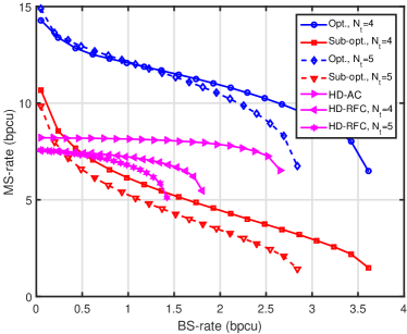
Figure 2: Comparison of rate regions with $P=0$ dBm, $\sigma^{2}_{h_{b}}=\sigma^{2}_{h_{m}}=30$ dBm and $N_{t}=4,5$.

It can be observed from Figs. 2 and 3 that the maximum value of the MS rate (in bits per channel use (bpcu)) is obtained when $R_{B}$ is minimum, whereas the minimum value is obtained when $R_{B}$ takes maximum value. Moreover, as expected both the BS and MS rates increase when $P$ increases from $0$ dBm to $10$ dBm. Both figures show that the optimum method performs significantly better than the sub-optimum approach. In the proposed optimum method, when $N_{t}$ increases, the obtained maximum MS rate increases, whereas the obtained maximum BS rate decreases. This can be explained from the fact that increasing $N_{t}$ improves the transmit beamforming at the BS, which in turn is attributed for an increase in the MS rate. However, increase in $N_{t}$ decreases $N_{r}=N-N_{t}$ for a given $N_{t}$. This means that the LI rejection capability of the BS decreases which leads to a drop in the supported BS rate. All results also show that the proposed optimum method significantly outperforms HD modes that employ both AC and RFC approaches. It is worthwhile to note that the boundaries of the MS-BS rate-regions remain relatively flat in the HD modes, although the corresponding maximum values of the BS and MS rates are smaller than those in the optimum and sub-optimum cases. When compared to the less expensive HD-RFC scheme, the sub-optimum method can be considered to provide a more flexible design. For example, in Fig. 2, the HD-RFC, with $N_{t}=4$, gives the maximum BS-rate of about 1.8 bpcu. The corresponding MS-rate is about 5.5 bpcu which drops to zero beyond the BS-rate of 1.8 bpcu. However, the corresponding sub-optimum scheme supports the BS-rate up to 3.6 bpcu, although this is achieved with the MS-rate of only about 1.5 bpcu.

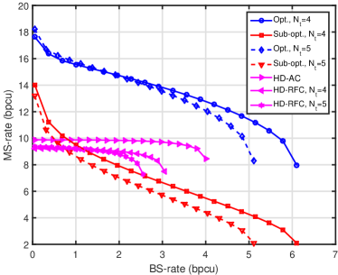
Figure 3: Comparison of rate regions with $P=10$ dBm, $\sigma^{2}_{h_{b}}=\sigma^{2}_{h_{m}}=30$ dBm, and $N_{t}=4,5$.

The rate regions of the optimum and sub-optimum methods with different values of $N_{t}$ are shown in Fig. 4 and Fig. 5 for $P=0$ dBm and $P=10$ dBm, respectively. From these figures, similar observations can be made as in Figs. 2 and 3.

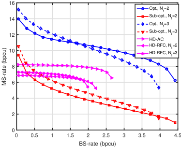
Figure 4: Comparison of rate regions with $P=0$ dBm, $\sigma^{2}_{h_{b}}=\sigma^{2}_{h_{m}}=30$ dBm, and $N_{t}=2,3$.

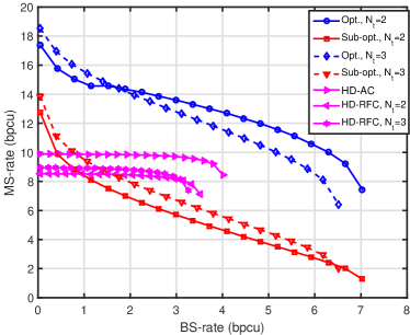
Figure 5: Comparison of rate regions $P=10$ dBm, $\sigma^{2}_{h_{b}}=\sigma^{2}_{h_{m}}=30$ dBm, and $N_{t}=2,3$.

V-B Partial CSI

In this subsection, we first compare the analytical expressions of the BS outage probability and ergodic MS rate with the simulations. Considering that the BS and MS are often surrounded by multiple scatterers and the angle of arrival/departure undergo some spreading, the spatial covariance matrices ${\bf R}_{B}$ and ${\bf R}_{M}$ are modeled according to [41] as

$$[{\bf R}_{B/M}]_{m,n}=\frac{{\rm e}^{{\rm j}\pi(m-n)\sin\theta_{B/M}}}{d^{\tau}}{\rm e}^{-\left(\pi(m-n)\sigma_{\theta}^{B/M}\cos\theta_{B/M}\right)^{2}/2},$$

where $[{\bf X}]_{m,n}$ denotes the $(m,n)$-th element of the matrix ${\bf X}$, $\theta_{B/M}$ is the central angle of the outgoing/incoming rays from/to the $N_{t}$ transmit/$(N-N_{t})$ receive antennas of the BS and $\sigma_{\theta}^{B/M}$ is the standard deviation of the corresponding angular spread. The comparisons between analytical and simulation results are shown in Figs. 6 and 7. In Fig. 6, we take $\sigma_{\theta}^{M}=10^{\circ}$, $\theta_{M}=15^{\circ}$, $\gamma_{B}=10$ bpcu, and vary $P$. In Fig. 7, $\sigma_{\theta}^{B}=10^{\circ}$, $\theta_{B}=5^{\circ}$, and $\sigma^{2}_{h_{b}}=30$ dBm are taken, and $\sigma^{2}_{h_{m}}$ is varied. A randomly selected unit beamformer is used in both figures and $\alpha=0.1$ is chosen.

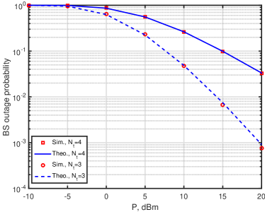
Figure 6: Comparison of analytical and simulated BS outage probability.

It can be observed from Fig. 6 that there is a good matching between the simulated and the analytical outage probability of the BS. Similarly, Fig. 7 shows that the simulated and theoretical results of the ergodic information rates at the MS exhibit also very good matching. Thus, these results verify the accuracy of the derived analytical expressions of outage probability and ergodic rate.

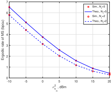
Figure 7: Ergodic MS rate versus variance of LI channel at the MS.

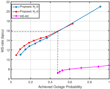
Figure 8: Ergodic MS rate versus BS outage probability for $N_{t}=2,N_{t}=3$, $N=6$, $P=10$ dBm, $\sigma^{2}_{h_{b}}=\sigma^{2}_{h_{m}}=30$ dBm, $\gamma_{B}=3$ bpcu.

The ergodic MS-rate versus BS outage probability is depicted in Figs. 8 and Figs. 9 for different values of $N_{t}$. In both figures, we take $\sigma_{\theta}^{B}=\sigma_{\theta}^{M}=10^{\circ}$, $\theta_{B}=5^{\circ}$, $\theta_{M}=15^{\circ}$. In Fig. 8, $P=10$ dBm and $\gamma_{B}=3$ bpcu are taken, whereas in Fig. 9, $P=0$ dBm and $\gamma_{B}=1$ bpcu are taken. The performance of the proposed FD scheme is compared with that of the HD-AC scheme in these figures.

It can be observed from these figures that the MS-rate has to be sacrificed for achieving lower outage probability at the BS. Moreover, from the results of Figs. 8 and 9, we observe that the MS rate drops whereas the outage probability improves when $N_{t}$ decreases (or $N-N_{t}$ increases). This is due to the fact that smaller $N_{t}$ decreases beamforming gain of the BS towards the MS, whereas the resulting larger value of $N-N_{t}$ increases the LI suppression capability of the BS. Both figures also demonstrate that the proposed FD scheme significantly outperforms the benchmark HD-AC scheme, despite the fact that the former scheme requires only half of the RF chains than in the latter.

For example, in Fig. 8, the achieved minimum outage probability with the HD-AC scheme is only about 0.47, whereas that achieved with the proposed method (with $N_{t}=2$) is approx. $0.05$ (improvement by a factor of 10). At the outage probability of 0.47, the HD-AC method achieves the MS-rate of only 7.2 bpcu, whereas the corresponding rate in the proposed scheme is about 10.9 bpcu. Similarly, in Fig. 9, the proposed scheme achieves the minimum outage probability of 0.017 (with $N_{t}=2$), whereas the HD-AC scheme achieves only 0.06. At this outage probability, the rate of the HD is 4.28 bpcu, whereas the corresponding rate of the proposed method is 7.05 bpcu.

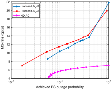
Figure 9: Ergodic MS rate versus BS outage probability for $N_{t}=2,3$, $N=6$, $P=0$ dBm, $\sigma^{2}_{h_{b}}=\sigma^{2}_{h_{m}}=30$ dBm, $\gamma_{B}=1$ bpcu.

VI Conclusions

In this paper, the joint optimization of transmit beamforming and TS parameter was considered for a wireless-powered bidirectional FD communication system. When instantaneous CSI is available, the boundary of the MS-BS information rate was obtained by efficiently solving the optimization problem as an SDR problem, in which the optimality of the relaxation was analytically confirmed. A sub-optimum approach based on zero-forcing constraint was also proposed, where a closed-form expression for TS parameter was also determined. When the BS and MS have only second-order statistics of their transmit CSI, the joint optimization was formulated as a problem of maximizing the ergodic MS rate, while satisfying the constraint on the BS outage probability. Utilizing the monotonicity property of the ergodic MS-rate and an upper bound of the outage probability, an SDR-based optimization problem was formulated and efficiently solved. Simulations demonstrate that significant performance gains are achievable over the half-duplex scheme when the beamformer and the TS parameter are jointly optimized.

Appendix A

Derivation of $R_{B}^{\rm max}$

It is obvious that

$$\|{\bf h}_{M}\|^{2}-\frac{|{\bf h}_{M}^{H}{\bf H}_{B}{\bf w}_{B}|^{2}}{\sigma_{b}^{2}+\|{\bf H}_{B}{\bf w}_{B}\|^{2}}\leq\|{\bf h}_{M}\|^{2},$$ (59)

where the equality is achieved with the ZF constraint ${\bf h}_{M}^{H}{\bf H}_{B}{\bf w}_{B}=0$. The maximum BS rate is then obtained as

$$R_{B}^{\rm max}=\max_{0<\alpha<1}(1-\alpha)\log_{2}\left(1+\frac{\alpha}{1-\alpha}b\frac{\|{\bf h}_{M}\|^{2}}{\sigma_{b}^{2}}\right),$$ (60)

where $b=\eta P{\bar{\lambda}}\left({\bf H}_{BM}{\bf H}_{BM}^{H}\right)$. Denote ${\tilde{b}}=b\frac{\|{\bf h}_{M}\|^{2}}{\sigma_{b}^{2}}$. Equating the first order derivative of $R_{B}^{\rm max}$ w.r.t. $\alpha$, we obtain

$$\frac{\partial R_{B}^{\rm max}}{\partial\alpha}=0\Longrightarrow\log\left(1+\frac{\alpha}{1-\alpha}{\tilde{b}}\right)=\frac{{\tilde{b}}}{1+\frac{\alpha}{1-\alpha}{\tilde{b}}}\frac{1}{1-\alpha},$$ (61)

which can be written in the form

$$z\log(z)=z+{\tilde{b}}-1,~{}{\rm where}~{}z=1+\frac{\alpha}{1-\alpha}{\tilde{b}}.$$ (62)

After some straightforward manipulations, we obtain

$$\frac{z}{{\rm e}}\log\left(\frac{z}{\rm e}\right)=\frac{{\tilde{b}}-1}{{\rm e}}\Longrightarrow\log\left(\frac{z}{{\rm e}}\right){\rm e}^{\log\left(\frac{z}{{\rm e}}\right)}=\frac{{\tilde{b}}-1}{{\rm e}}.$$ (63)

According to the definition of Lambert-W function [33], the solution of the equation $y=xe^{x}$ for a given $y$ is expressed as $x=W(y)$, where $W(\cdot)$ is the Lambert-W function. Thus, (63) is given by

$$z={\rm e}^{W\left(\frac{{\tilde{b}}-1}{{\rm e}}\right)+1}.$$ (64)

Substituting $z$ into (64), the optimum $\alpha$ is

$$\alpha^{\rm Opt}=\frac{{\rm e}^{W\left(\frac{{\tilde{b}}-1}{{\rm e}}\right)+1}-1}{{\tilde{b}}+{\rm e}^{W\left(\frac{{\tilde{b}}-1}{{\rm e}}\right)+1}-1}.$$ (65)

Therefore, $R_{B}^{\rm max}$ is given by

$$R_{B}^{\rm max}=(1-\alpha^{\rm Opt})\log_{2}\left(1+\frac{\alpha^{\rm Opt}}{1-\alpha^{\rm Opt}}\frac{b\|{\bf h}_{M}\|^{2}}{\sigma_{b}^{2}}\right).$$ (66)

Appendix B

Proof of Proposition  1

The Lagrangian multiplier function for the optimization problem (III-A1) is

$${\mathcal{L}}({\bf V}_{B},{\bf Y},\lambda_{1},\lambda_{2}) = -{\rm tr}({\bf V}_{B}{\bf h}_{B}{\bf h}_{B}^{H})-{\rm tr}({\bf Y}{\bf V}_{B})$$ (67)

$$+\lambda_{1}\left[{\rm tr}\left({\bf V}_{B}{\bf H}_{B}^{H}\left({\bf h}_{M}{\bf h}_{M}^{H}-\Gamma_{B}{\bf I}\right){\bf H}_{B}\right)\right]$$

$$+\lambda_{2}\left({\rm tr}({\bf V}_{B})-P\right)-\lambda_{1}\sigma_{b}^{2}\Gamma_{B},$$

where ${\bf Y}\succeq 0$ is the dual-variable associated with the positive semidefinite constraint ${\bf V}_{B}\succeq 0$, and $\lambda_{1}\geq 0$ & $\lambda_{2}\geq 0$ are the Lagrangian multiplier coefficients. Among all KKT conditions, some relevant conditions required for the proof are as follows.

$$\frac{d{\mathcal{L}}}{d{\bf V}_{B}} = \biggl{\{}-{\bf h}_{B}{\bf h}_{B}^{H}+\lambda_{1}{\bf H}_{B}^{H}\left({\bf h}_{M}{\bf h}_{M}^{H}-\Gamma_{B}{\bf I}\right){\bf H}_{B}\biggr{.}$$

. $$+\lambda_{2}{\bf I}-{\bf Y}\biggr{\}}={\bf 0}$$ (68)

$${\rm tr}({\bf Y}{\bf V}_{B}) = 0\Longrightarrow{\bf Y}{\bf V}_{B}={\bf 0},~{}{\bf V}_{B}\succeq 0,{\bf Y}\succeq 0.$$ (69)

The KKT condition (69) implies that the optimum ${\bf V}_{B}$ must lie in the null-space of ${\bf Y}$. This means that the rank of optimum ${\bf V}_{B}$ is the nullity of ${\bf Y}$. Consequently, it is sufficient to show that the optimum ${\bf Y}$ has a nullity of one. Note that $\Gamma_{B}\geq 0$ and

$${\bf Y}=-{\bf h}_{B}{\bf h}_{B}^{H}+\lambda_{1}\left[{\bf H}_{B}^{H}\left({\bf h}_{M}{\bf h}_{M}^{H}-\Gamma_{B}{\bf I}\right){\bf H}_{B}\right]+\lambda_{2}{\bf I}.$$ (70)

Define ${\bf Z}\triangleq\lambda_{1}\left[{\bf H}_{B}^{H}\left({\bf h}_{M}{\bf h}_{M}^{H}-\Gamma_{B}{\bf I}\right){\bf H}_{B}\right]+\lambda_{2}{\bf I}$. We first claim that at the KKT optimality, ${\bf Z}$ is a positive-definite (full- rank) matrix. This can be readily proved by the method of contradiction. Consider the cases where ${\bf Z}$ has at least one non-positive eigenvalue. Then, from Weyl’s inequalities for sum of eigenvalues of Hermitian matrices [27], it is clear that ${\bf Z}-{\bf h}_{B}{\bf h}_{B}^{H}$ will have at least one negative eigenvalue. In other words, ${\bf Y}$ turns to a indefinite matrix, which contradicts the fact that ${\bf Y}$ should be positive-semidefinite. Consequently, positive-semidefiniteness of ${\bf Y}$ can be confirmed only when ${\bf Z}$ is positive-definite. Now, we can show that the nullity of ${\bf Y}$ cannot be greater than 1 by contradiction. Assume that $\left\{{\bf u}_{y,q},q=1,2\right\}\in{\mathcal{N}s}({\bf Y})$, where ${\mathcal{N}s}({\bf Y})$ denotes null-space of ${\bf Y}$. Then,

$${\bf Y}{\bf u}_{y,q} = {\bf Z}{\bf u}_{y,q}-{\bf h}_{B}{\bf h}_{B}^{H}{\bf u}_{y,q}$$ (71)

$$\Longrightarrow{\bf 0}={\bf Z}{\bf u}_{y,q}-{\bf h}_{B}{\bf h}_{B}^{H}{\bf u}_{y,q}$$

$$\Longrightarrow{\bf u}_{y,q}={\bf Z}^{-1}{\bf h}_{B}{\bf h}_{B}^{H}{\bf u}_{y,q},\forall q,$$

which shows that ${\bf u}_{y,q}$ is an eigenvector of ${\bf Z}^{-1}{\bf h}_{B}{\bf h}_{B}^{H}$ corresponding to eigenvalue $1$. Since ${\rm rank}({\bf Z}^{-1}{\bf h}_{B}{\bf h}_{B}^{H})=1$, it turns out that $q$ cannot take a value greater than $1$. This shows that the dimension of null space of ${\bf Y}$ is one, and therefore, the rank of ${\bf V}_{B}$ is one. $\square$

Appendix C

Proof of Proposition  2

The equality constraint for the BS rate is expressed as

$$\log\left(1+\frac{\alpha}{1-\alpha}b\gamma\right)=R_{B}\log(2)\left(\frac{\alpha}{1-\alpha}+1\right).$$ (72)

Define $y\triangleq 1+\frac{\alpha}{1-\alpha}b\gamma$. Then (72) can be expressed in terms of $y$ as

$$y={\rm e}^{\frac{R_{B}\log(2)}{b\gamma}y}{\rm e}^{R_{B}\log(2)\left(1-\frac{1}{b\gamma}\right)},$$ (73)

which after simple manipulation can be expressed as

$$\left(-\frac{R_{B}\log(2)}{b\gamma}y\right){\rm e}^{-\frac{R_{B}\log(2)}{b\gamma}y} = \left(-\frac{R_{B}\log(2)}{b\gamma}\right)$$ (74)

$$\times{\rm e}^{R_{B}\log(2)\left(1-\frac{1}{b\gamma}\right)}.$$

Using the Lambert-W function $W(y)$ (i.e., $y=x{\rm e}^{x}\rightarrow x=W(y)$), $y$ in (74) is expressed as

$$y=\frac{-b\gamma}{R_{B}\log(2)}W\left(-\frac{R_{B}\log(2)}{b\gamma}{\rm e}^{R_{B}\log(2)\left(1-\frac{1}{b\gamma}\right)}\right).$$ (75)

Note that $\frac{R_{B}\log(2)}{b\gamma}{\rm e}^{R_{B}\log(2)\left(1-\frac{1}{b\gamma}\right)}\leq\frac{1}{\rm e}$ is required to have a real value of $y$. If not, the equality constraint is not feasible for given $b$, $\gamma$, and $R_{B}$ where $R_{B}\leq R_{B}^{\rm max}$. Substituting $y$ in (75), we obtain

$$\frac{\alpha}{1-\alpha}=\frac{-1}{R_{B}\log(2)}W\left(-\frac{R_{B}\log(2)}{b\gamma}{\rm e}^{R_{B}\log(2)\left(1-\frac{1}{b\gamma}\right)}\right)-\frac{1}{b\gamma},$$

which yields the optimum ${\bar{\alpha}}^{\rm Opt}$ given in (24). $\square$

Appendix D

Proof of Proposition 3

Let ${\bar{z}}={\bf h}_{M}^{H}\left(\sigma_{b}^{2}{\bf I}+{\bf H}_{B}{\bf w}_{B}{\bf w}_{B}^{H}{\bf H}_{B}\right)^{-1}{\bf h}_{M}$. Since ${\bf h}_{M}={\bf R}_{M}^{\frac{1}{2}}{\bf h}_{M,w}$, where we consider that the effect of the distance dependent attenuation is included in ${\bf R}_{M}$.

$${\bar{z}}={\bf h}_{M,w}^{H}\underbrace{{\bf R}_{M}^{\frac{1}{2}}\left(\sigma_{b}^{2}{\bf I}+{\bf H}_{B}{\bf w}_{B}{\bf w}_{B}^{H}{\bf H}_{B}\right)^{-1}{\bf R}_{M}^{\frac{1}{2}}}_{{\bm{\Phi}}}{\bf h}_{M,w}.$$ (76)

Let the eigenvalue decomposition of ${\bm{\Phi}}$ be given by ${\bm{\Phi}}={\bf U}{\bm{\Lambda}}{\bf U}^{H}$, where ${\bm{\Lambda}}$ is the diagonal matrix of eigenvalues of ${\bm{\Phi}}$, whereas ${\bf U}$ is the matrix of eigenvectors. Let $\{\lambda_{i}\}_{i=1}^{L}$ be the non-zero eigenvalues of ${\bm{\Phi}}$, where its rank is $L$. Then, (76) is further expressed as

$${\bar{z}} = {\bf h}_{M,w}^{H}{\bf U}{\bm{\Lambda}}{\bf U}^{H}{\bf h}_{M,w}={\tilde{\bf h}}_{M,w}^{H}{\bm{\Lambda}}{\tilde{\bf h}}_{M,w}$$ (77)

$$= \sum_{i=1}^{L}\lambda_{i}|{\tilde{h}}_{M,w,i}|^{2},$$

where ${\tilde{\bf h}}_{M,w}={\bf U}^{H}{\bf h}_{M,w}$ and ${\tilde{h}}_{M,w,i}$ is the $i$th element of ${\tilde{\bf h}}_{M,w}$. Since ${\bf U}$ is a unitary matrix, the elements of ${\tilde{\bf h}}_{M,w}$ remain ZMCSCG as the elements of ${\bf h}_{M,w}$. The outage probability at the BS is given by

$$P_{out,B}={\rm Pr}\left\{(1-\alpha)\log_{2}(1+p_{m}{\bar{z}})\leq\gamma_{B}\right\},$$ (78)

which after applying (77) gives

$$P_{out,B} = {\rm Pr}\left\{\sum_{i=1}^{L}\lambda_{i}|{\tilde{h}}_{M,w,i}|^{2}\leq\frac{1}{p_{m}}\left[2^{\frac{\gamma_{B}}{1-\alpha}}-1\right]\right\}$$ (79)

$$= {\rm Pr}\left\{\sum_{i=1}^{L}\lambda_{i}|{\tilde{h}}_{M,w,i}|^{2}\leq{\bar{\gamma}}\right\}.$$

Since ${\tilde{h}}_{M,w,i}$ is ZMCSCG with unit variance, $|{\tilde{h}}_{M,w,i}|^{2}$ is exponentially distributed with unit parameter. Then, the RV $X=\sum_{i=1}^{L}\lambda_{i}|{\tilde{h}}_{M,w,i}|^{2}$ is a weighted sum of independent exponentially distributed random variables. The PDF of $X$ is given by [43, p.11]

$$f_{X}(x)=\sum_{i=1}^{L}a_{i}{\rm e}^{\displaystyle{-\frac{x}{\lambda_{i}}}},$$ (80)

where $x\geq 0$, and for $L>1$

$$a_{i}=\frac{\lambda_{i}^{L-2}}{\prod_{j=1,j\neq i}^{L}\lambda_{i}-\lambda_{j}}.$$ (81)

For $L=1$, $a_{i}$ takes the values of $\frac{1}{\lambda_{i}}$. Substituting the PDF of $X$ into (79), we get

$$P_{out,B}=\int_{0}^{\bar{\gamma}}f_{X}(x)\,dx = \sum_{i=1}^{L}a_{i}\int_{0}^{\bar{\gamma}}{\rm e}^{-\frac{x}{\lambda_{i}}}\,dx$$ (82)

$$= \sum_{i=1}^{L}a_{i}\lambda_{i}\left[1-{\rm e}^{-\frac{{\bar{\gamma}}}{\lambda_{i}}}\right]$$

which completes the proof. $\square$

References

- [1] A. Sabharwal, P. Schniter, D. Guo, D. W. Bliss, S. Rangarajan and R. Wichman, “In-band full-duplex wireless: Challenges and opportunities,” IEEE J. Sel. Areas Commun., vol. 32, pp. 1637-1652, Sept. 2014.
- [2] Z. Zhang, K. Long, A. V. Vasilakos and L. Hanzo, “Full-duplex wireless communications: Challenges, solutions, and future research directions,” Proc. IEEE, vol. 104, pp. 1369-1409, July 2016.
- [3] J. I. Choi, M. Jain, K. Srinivasan, P. Levis, and S. Katti, “Achieving single channel, full duplex wireless communication,” in Proc. 16th Annual Intl. Conf. Mobile Computing and Networking (Mobicom 2010), Chicago, IL, Sep. 2010, pp. 1-12.
- [4] T. Riihonen, S. Werner, and R. Wichman, “Hybrid full-duplex/half-duplex relaying with transmit power adaptation,” IEEE Trans. Wireless Commun., vol. 10, pp. 3074-3085, Sep. 2011.
- [5] T. Riihonen, S. Werner, and R. Wichman, “Mitigation of loopback self-interference in full-duplex MIMO relays,” IEEE Trans. Signal Process., vol. 59, pp. 5983-5993, Dec. 2011.
- [6] M. Duarte, C. Dick, and A. Sabharwal, “Experiment-driven characterization of full-duplex wireless systems,” IEEE Trans. Wireless Commun., vol. 11, pp. 4296-4307, Dec. 2012.
- [7] D. Korpi, M. Heino, C. Icheln, K. Haneda and M. Valkama, “Compact inband full-duplex relays with beyond 100 dB self-interference suppression: Enabling techniques and field measurements,” IEEE Trans. Antennas Propag., vol. 65, no. 2, pp. 960-965, Feb. 2017.
- [8] H. Q. Ngo, H. A. Suraweera, M. Matthaiou and E. G. Larsson, “Multipair full-duplex relaying with massive arrays and linear processing,” IEEE J. Sel. Areas Commun., vol. 32, pp. 1721-1737, Sept. 2014.
- [9] D. Senaratne and C. Tellambura, “Beamforming for space division duplexing,” in Proc. IEEE Intl. Conf. Commun. (ICC 2011), Kyoto, Japan, June 2011, pp. 1-5.
- [10] B. P. Day, A. R. Margetts, D. W. Bliss, and P. Schniter, “Full-duplex bidirectional MIMO: Achievable rates under limited dynamic range,” IEEE Trans. Signal Process., vol. 60, pp. 3702-3713, July 2012.
- [11] H. Ju, X. Shang, H. V. Poor and D. Hong, “Bi-directional use of spatial resources and effects of spatial correlation,” IEEE Trans. Wireless Commun., vol. 10, pp. 3368-3379, Oct. 2011.
- [12] A. C. Cirik, Y. Rong and Y. Hua, “Achievable rates of full-duplex MIMO radios in fast fading channels with imperfect channel estimation,” IEEE Trans. Signal Process., vol. 62, pp. 3874-3886, Aug. 2014.
- [13] X. Lu, P. Wang, D. Niyato, D. I. Kim and Z. Han, “Wireless networks with RF energy harvesting: A contemporary survey,” IEEE Commun. Surv. Tut., vol. 17, pp. 757-789, Second quarter 2015.
- [14] S. Bi, Y. Zeng, and R. Zhang, “Wireless powered communication networks: An overview,” Wireless Commun., vol. 23, pp. 10-18, Apr. 2016.
- [15] K. Huang and V. K. N. Lau, “Enabling wireless power transfer in cellular networks: Architecture, modeling and deployment,” IEEE Trans. Wireless Commun., vol. 13, pp. 6499-6514, Feb. 2014.
- [16] R. Zhang and C. Ho, “MIMO broadcasting for simultaneous wireless information and power transfer,” IEEE Trans. Wireless Commun., vol. 12, pp. 1989-2001, May 2013.
- [17] W. Huang, H. Chen, Y. Li and B. Vucetic, “On the performance of multi-antenna wireless-powered communications with energy beamforming,” IEEE Trans. Veh. Technol., vol. 65, pp. 1801-1808, Mar. 2016.
- [18] H. Ju and R. Zhang, “Optimal resource allocation in full-duplex wireless powered communication network,” IEEE Trans. Commun., vol. 62, pp. 3528-3540, Oct. 2014.
- [19] K. Yamazaki, Y. Sugiyama, Y. Kawahara, S. Saruwatari and T. Watanabe, “Preliminary evaluation of simultaneous data and power transmission in the same frequency channel,” in Proc. IEEE WCNC 2015, New Orleans, LA, Mar. 2015, pp. 1-6.
- [20] M. Gao, H. H. Chen, Y. Li, M. Shirvanimoghaddam and J. Shi, “Full-duplex wireless-powered communication with antenna pair selection,” in Proc. IEEE WCNC 2015, New Orleans, LA, 2015, pp. 693-698.
- [21] Z. Hu, C. Yuan, F. Zhu, and F. Gao, “Weighted sum transmit power minimization for full-duplex system with SWIPT and self-energy recycling,” IEEE Access, vol. 4, pp. 4874-4881, 2016.
- [22] Z. Ding, C. Zhong, D. W. K. Ng, M. Peng, H. A. Suraweera, R. Schober and H. V. Poor, “Application of smart antenna technologies in simultaneous wireless information and power transfer,” IEEE Commun. Mag., vol. 53, pp. 86-93, Apr. 2015.
- [23] B. K. Chalise, H. A. Suraweera, and G. Zheng, “Throughput maximization for full-duplex energy harvesting MIMO communications,” in Proc. IEEE SPAWC 2016, Edinburgh, UK, June 2016, pp. 1-5.
- [24] A. Masmoudi, and T. Le-Ngoc, “Residual self-interference after cancellation in full-duplex systems,” in Proc. IEEE Intl. Conf. Commun., (ICC 2014), Sydney, Australia, June 2014, pp. 4680-4685.
- [25] M. Mohammadi, B. K. Chalise, H. A. Suraweera, C. Zhong, G. Zheng, and I. Kirkidis, “Throughput analysis and optimization of wireless-powered multiple antenna full-duplex relay systems,” IEEE Trans. Commun., vol. 64, pp. 1769 - 1785, Apr. 2016.
- [26] Y. Zeng, B. Clerckx, and R. Zhang, “Communications and signals design for wireless power transmission,” IEEE Trans. Commun., vol. PP, no. 99, pp. 1-1. [Online]. Available: https://arxiv.org/pdf/1611.06822.pdf.
- [27] R. A. Horn and C. A. Johnson, Matrix Analysis, 2nd ed., New York, NY: Cambridge University Press, 2013.
- [28] W. W. Hager, “Updating the inverse of a matrix,” SIAM Review, vol. 31, pp. 221-239, June 1989.
- [29] S. Boyd and L. Vandenberghe, Convex Optimization, Cambridge University Press, 2004.
- [30] Z. Q. Luo, W. K. Ma, A. M. C. So, Y. Ye, and S. Zhang, “Semidefinite relaxation of quadratic optimization problems,” IEEE Signal Process. Mag., vol. 27, no. 3, pp. 20-34, May 2010.
- [31] F. Zhu, F. Gao, T. Zhang, K. Sun, and M. Yao, “Physical-layer security for full duplex communications with self-interference mitigation,” IEEE Trans. Wireless Commun., vol. 15, no. 1, pp. 329-340, Jan. 2016.
- [32] H. A. Suraweera, I. Krikidis, G. Zheng, C. Yuen and P. J. Smith, “Low-complexity end-to-end performance optimization in MIMO full-duplex relay systems,” IEEE Trans. Wireless Commun., vol. 13, pp. 913-927, Feb. 2014.
- [33] R. M. Corless, G. H. Gonnet, D. E. G. Hare, D. J. Jeffrey, and D. E. Knuth, “On the Lambert W function,” Advances in Computational Mathematics, vol. 5, pp. 329-359, 1996.
- [34] S. Barghi, A. Khojastepour, K. Sundaresan, and S. Rangarajan, “Characterizing the throughput gain of single cell MIMO wireless systems with full duplex radios,” in Proc. 10th Int. Symp. Modeling and Optimization in Mobile, Ad Hoc and Wireless Networks (WiOpt), Padeborn, Germany, May 2012.
- [35] S. Zhou and G. B. Giannakis, “Optimal transmitter eigen-beamforming and space-time block coding based on channel correlations,” IEEE Trans. Inf. Theory, vol. 49, pp. 1673-1690, July 2002.
- [36] B. K. Chalise, W.-K., Ma, Y. D. Zhang, H. A. Suraweera, and M. G. Amin, “Optimum performance boundaries of OSTBC based AF-MIMO relay system with energy harvesting receiver,” IEEE Trans. Signal Process., vol. 61, no. 17. pp. 4199-4213, Sept. 2013.
- [37] I. S. Gradshteyn and I. M. Ryzhik, Table of Integrals, Series, and Products. 7th ed., San Diego, CA: Academic Press, 2007.
- [38] M. Abramowitz and I. A. Stegun, Handbook of Mathematical Functions With Formulas, Graphs, and Mathematical Tables. 9th ed., New York: Dover, 1970.
- [39] M. K. Simon and M.-S. Alouini, Digital communications over fading channels. 2nd ed., New York, NY: John Wiley & Sons, 2005.
- [40] B. K. Chalise and L. Vandendorpe. “MIMO relay design for multipoint-to-multipoint communications with imperfect channel state information,” IEEE Trans. Signal Process., vol. 57, pp. 2785-2796, July 2009.
- [41] M. Bengtsson and B. Ottersten, “Optimum and sub-optimum transmit beamforming,” Handbook of Antennas in Wireless Communications, Boca Raton, FL: CRC Press, 2001.
- [42] D. Bharadia, E. McMilin, and S. Katti, “Full duplex radios”, Proc. ACM SIGCOMM 2013, Hong Kong, China, Aug. 2013, pp. 375-386.
- [43] D. R. Cox, Renewal Theory, London: Methuen’s Monographs on Applied Probability and Statistics, 1967.