Quantum phase transition and unusual critical behavior in multi-Weyl semimetals

Abstract

The low-energy behaviors of gapless double- and triple-Weyl fermions caused by the interplay of long-range Coulomb interaction and quenched disorder are studied by performing a renormalization group analysis. It is found that an arbitrarily weak disorder drives the double-Weyl semimetal to undergo a quantum phase transition into a compressible diffusive metal, independent of the disorder type and the Coulomb interaction strength. In contrast, the nature of the ground state of triple-Weyl fermion system relies sensitively on the specific disorder type in the noninteracting limit: The system is turned into a compressible diffusive metal state by an arbitrarily weak random scalar potential or $z$ component of random vector potential but exhibits stable critical behavior when there is only $x$ or $y$ component of random vector potential. In case the triple-Weyl fermions couple to random scalar potential, the system becomes a diffusive metal in the weak interaction regime but remains a semimetal if Coulomb interaction is sufficiently strong. Interplay of Coulomb interaction and $x$, or $y$, component of random vector potential leads to a stable infrared fixed point that is likely to be characterized by critical behavior. When Coulomb interaction coexists with the $z$ component of random vector potential, the system flows to the interaction-dominated strong coupling regime, which might drive a Mott insulating transition. It is thus clear that double- and triple-Weyl fermions exhibit distinct low-energy behavior in response to interaction and disorder. The physical explanation of such distinction is discussed in detail. The role played by long-range Coulomb impurity in triple-Weyl semimetal is also considered. The main conclusion is that, Coulomb impurity always drives the system to become a compressible diffusive metal, whereas Coulomb interaction tends to suppress the Coulomb impurity, rendering the robustness of the semimetal phase.

I Introduction

Topological semimetals (SMs), including Dirac semimetal (DSM) Vafek14 ; Wehling14 ; Armitage17 , Weyl semimetal (WSM) Armitage17 ; Wan11 ; Burkov16 ; Yan17 ; Hasan17 , and nodal line semimetal (NLSM) Armitage17 ; Weng16 ; FangChen16 , have attracted broad research interest among the condensed-matter community. These materials exhibit many intriguing properties, provide ideal platforms for exploring some important physical concepts, and also have promising industrial applications. Specifically, WSM has been theoretically predicted and experimentally observed in the TaAs family Huang15 ; WengHM15 ; Xu15A ; Lv15A . In usual WSMs, the fermion excitations emerge at low energies from pairs of Weyl nodes with opposite monopole charges $\pm 1$, and have a linear-in-momentum dispersion Wan11 ; Burkov16 ; Yan17 . They are known to host symmetry-protected Fermi arc surface states Wan11 ; Burkov16 ; Yan17 and display chiral anomaly that is related to the presence of negative magnetoresistance HuangChenGFGroup15 ; ZhangChengLong16 . Apart from usual WSMs, there are also multi-WSMs in which the monopole charges of Weyl nodes can be larger than unity XuFang11 ; Fang12 ; YangNogasa14 ; Bradlyn16 ; Gao16 ; Huang16 ; Guan15 ; LiuZunger17 ; ChenChan16 ; ChangChan17 ; Lai15 ; Jian15 ; Zhang16 ; WangLiuZhang16 ; Jian16 ; Goswami15 ; Roy15 ; BeraRoy16 ; LiRoy16 ; Roy17 ; Ahn16 ; Ahn17 ; Park17 ; Huang17 ; Hayata17 ; Sun17 ; Shapourian16 ; Sbierski17 . Two known examples are double- and triple-WSMs, where the fermion dispersion is linear in one of the momentum components, but quadratic and cubic in the other two components. Accordingly, the monopole charges of double- and triple-Weyl fermions are $\pm 2$ and $\pm 3$, respectively.

Differen from ordinary metals that possess a finite Fermi surface, multi-WSMs have only zero-dimensional Fermi points. Accordingly, the density of states (DOS) vanishes at zero energy, i.e. $\rho(0)=0$, which renders the robustness of the long-range character of Coulomb interaction. The dynamics of multi-Weyl fermions are distinct from ordinary electrons when they are surrounded by a randomly distributed potential. The impact of Coulomb interaction Shankar94 ; ColemanBook ; Varma02 ; Kotov12 and disorder Lee85 ; Evers08 ; DasSarma11 ; Syzranov16Review on the low-energy behavior of multi-WSMs might be drastically different from normal metals. The purpose of the present paper is to give a comprehensive theoretic analysis of the low-energy behavior of double- and triple-WSMs in the presence of both Coulomb interaction and disorder.

Table 1: Summary of the possible ground states of double- and triple-WSMs due to the interplay between Coulomb interaction and disorder. Here, $\alpha_{0}$ is the bare strength parameter for Coulomb interaction. We use $\Delta_{00}$, $\Delta_{10}$, $\Delta_{20}$, and $\Delta_{30}$ to denote the bare disorder parameter for RSP, $x$-RVP, $y$-RVP, and $z$-RVP, respectively. Morever, CDM stands for compressive diffusive metal, SM for semimetal, and SCS for stable critical state.

	Double-Wely Semimetal		Triple-Weyl Semimetal
	$\alpha_{0}=0$	$\alpha_{0}>0$	$\alpha_{0}=0$	$\alpha_{0}>0$
$\Delta_{00}>0$	$\Delta_{0}\rightarrow\infty$ CDM	$\Delta_{0}\rightarrow\infty,\alpha\rightarrow\infty,\alpha/\Delta_{0}\rightarrow 0$ CDM	$\Delta_{0}\rightarrow\infty$ CDM	$\alpha_{0}<\alpha_{0c}(\Delta_{00})$	$\alpha_{0}>\alpha_{0c}(\Delta_{00})$
				$\alpha\rightarrow\infty$, $\Delta_{0}\rightarrow\infty$, $\alpha/\Delta_{0}\rightarrow 0$ CDM	$\alpha\rightarrow 0$, $\Delta_{0}\rightarrow 0$, $\Delta_{0}/\alpha\rightarrow 0$ SM
$\Delta_{10}>0$			$\Delta_{1}\rightarrow\Delta_{1}^{*}$ SCS	$\Delta_{1}\rightarrow\Delta_{1n}^{*},\alpha\rightarrow\alpha_{n}^{*}$ Possible SCS
$\Delta_{20}>0$			$\Delta_{2}\rightarrow\Delta_{2}^{*}$ SCS	$\Delta_{2}\rightarrow\Delta_{2n}^{*},\alpha\rightarrow\alpha_{n}^{*}$ Possible SCS
$\Delta_{30}>0$			$\Delta_{3}\rightarrow\infty$ CDM	$\Delta_{3}\rightarrow\infty,\alpha\rightarrow\infty,\alpha/\Delta_{3}>1$ Possible Mott Insulator

Previous renormalization group (RG) studies Lai15 ; Jian15 showed that the Coulomb interaction in clean double-WSMs is marginally irrelevant, which results in logarithmic-like corrections for some observable quantities. The RG analysis of Zhang et al. Zhang16 found that the Coulomb interaction is also marginally irrelevant in clean triple-WSMs. In a recent work WangLiuZhang16 , we carried out a RG study of the quasiparticle residue $Z_{f}$ and the Landau damping rate after including the energy dependence of dressed Coulomb interaction, and illustrated that the conventional Fermi liquid (FL) description is spoiled in both double- and triple-WSMs in an anomalous manner. In particular, though the Coulomb interaction only leads to a relatively weak Landau damping effect, the residue $Z_{f}$ vanishes in the lowest energy limit, resulting in a new type of non-Fermi liquid (NFL) state. In such a NFL state, the FL theory is violated more weakly than a marginal Fermi liquid (MFL), which has long been regarded as the weakest breakdown of FL theory Varma02 .

The disorder effects on non-interacting double-Weyl fermions have been studied by means of several methods, including self-consistent Born approximation (SCBA) Goswami15 , RG approach BeraRoy16 , and large-scale quantum simulations Sbierski17 . It was showed BeraRoy16 ; Syzranov16Review ; Fradkin86 ; Goswami11 ; Kobayashi14 ; Sbierski14 ; Roy14 ; Syzranov15A ; Syzranov15B ; Pixley15 ; Sbierski15 ; Roy16Erratum ; Liu16 ; Roy16A ; Syzranov16A ; Louvet16 ; Pixley16A ; Pixley16B ; Pixley16C ; Roy16B ; Roy16C ; Sbierski16 ; Fu17 ; Pixley17 that even an arbitrarily weak disorder is able to drive the double-WSM to enter into a compressible diffusive metal (CDM) phase (see, however, Ref. Shapourian16 ), which is characterized by the generation of finite zero-energy disorder scatting rate $\gamma_{0}$ and finite zero-energy DOS $\rho(0)$. One might regard $\rho(0)$ as an effective order parameter for the CDM phase. Moreover, the electric conductivity is finite at zero temperature in this phase. A naive power counting suggests that short-range disorder is a relevant perturbation in a triple-WSM BeraRoy16 . However, a detailed RG analysis of disorder effects on triple-Weyl fermions is still lacking.

When both Coulomb interaction and disorder are considered, their interplay might give rise to a variety of intriguing properties Finkelstein84 ; Castellani84 ; PunnooseFinkelstein05 ; Abrahams01 ; Kravchenko04 ; Spivak10 ; Ye98 ; Ye99 ; Stauber05 ; Herbut08 ; Vafek08 ; Foster08 ; WangLiu14 ; Zhao16 ; Goswami11 ; Roy16A ; Gonzalez17 ; Moon14 ; Nandkishore17 ; YuXuanWang17 . This problem has been extensively studied for over three decades, and plays a vital role in the studies of two-dimensional (2D) metallic systems Finkelstein84 ; Castellani84 ; PunnooseFinkelstein05 ; Abrahams01 ; Kravchenko04 ; Spivak10 . It is believed by many researchers that the observed metal-insulator transition in some 2D systems is driven by an intricate interplay of strong Coulomb interaction and disorder scattering Finkelstein84 ; Castellani84 ; PunnooseFinkelstein05 ; Abrahams01 . Unfortunately, the progress of this subject is extremely slow, and there is still not an unified framework that treats the interplay of interaction and disorder in a satisfactory way.

Because of the peculiar geometry of Fermi surface of SMs, the interplay of Coulomb interaction and disorder may lead to distinct low-energy behavior comparing to traditional metals Ye98 ; Ye99 ; Stauber05 ; Herbut08 ; Vafek08 ; Foster08 ; Goswami11 ; WangLiu14 ; Zhao16 ; Roy16A ; Gonzalez17 ; Moon14 ; Nandkishore17 ; YuXuanWang17 . In this paper, we present a systematic RG study of the interplay of Coulomb interaction and quenched disorder, including random scalar potential (RSP) and random vector potential (RVP), in both double- and triple-WSMs. Normally, the Coulomb interaction tends to suppress the low-energy DOS of Dirac/Weyl fermions Vafek14 ; Wehling14 ; Kotov12 . In contrast, disorder can usually enhance the fermion DOS Kotov12 ; Evers08 ; DasSarma11 ; Syzranov16Review . The true low-energy dynamics of the fermions should be determined by an appropriate treatment of the mutual influence between interaction and disorder Ye98 ; Ye99 ; Stauber05 ; Herbut08 ; Vafek08 ; Foster08 ; Goswami11 ; WangLiu14 ; Moon14 ; Zhao16 ; Roy16A ; Gonzalez17 ; Nandkishore17 ; YuXuanWang17 . Our RG analysis reveals a remarkable difference between double- and triple-WSMs. In particular, we find that, an arbitrarily weak disorder is able to turn double-WSM into a CDM. It is important to notice that such a transition happens for any type of disordered potential and is independent of the Coulomb interaction strength. In sharp contrast to the double-WSM, the subtle interplay between Coulomb interaction and disorder can give rise to a variety of different ground states and various quantum phase transitions (QPT) in a triple-WSM, which is summarized in Table 1. In the non-interacting limit, the system is turned into a CDM phase by an arbitrarily weak RSP or $z$-component of RVP, dubbed $z$-RVP hereafter, but exhibits stable critical state when there is only $x$-RVP or $y$-RVP. In case the triple-Weyl fermions couple to RSP, the system becomes a CDM in the weak interaction regime, but is turned back to a SM if the Coulomb interaction becomes sufficiently strong. The interplay of Coulomb interaction and $x$-RVP, or $y$-RVP, produces a stable fixed point that is likely to be characterized by the emergence of unusual critical behavior. When Coulomb interaction coexists with $z$-RVP, the system flows to the interaction-dominated strong coupling regime, which might drive a Mott insulating transition. If two or more types of disorder coexist, triple-WSM is always driven to undergo a CDM transition, no matter the Coulomb interaction is included or not, which is similar to double-WSM.

All the above considerations are restricted to short-range disorder. In various SMs, there might be disorder with long-range correlation, such as Coulomb impurity. The long-range disorder may be more important than short-range disorder in SM systems. We will also apply the RG approach to study the interplay of long-range Coulomb interaction, long-range Coulomb impurity, and short-range RSP in triple-WSM. Our main conclusion is that, the Coulomb impurity can always drive a SM-to-CDM phase transition, whereas the Coulomb interaction tends to suppress the Coulomb impurity, rendering the robustness of the SM phase.

The rest of the paper is structured as follows. We present the effective action in Sec. II, and discuss the RG results in Sec. III. We address several related issues in Sec IV. The results are briefly summarized in Sec. V. The detailed derivations of the RG equations are presented in the Appendices.

II Effective action

The free Hamiltonian for double-Weyl fermions is Lai15 ; Jian15 ; Jian16 ; WangLiuZhang16 ; Zhang16

$$H_{d}=\int d^{3}\mathbf{x}\psi_{d}^{{\dagger}}(\mathbf{x})\left[Ad_{i}(\mathbf{x})\sigma_{i}-iv\partial_{z}\sigma_{3}\right]\psi_{d}(\mathbf{x}),$$ (1)

where $d_{1}(\mathbf{x})=-\left(\partial_{x}^{2}-\partial_{y}^{2}\right)$ and $d_{2}(\mathbf{x})=-2\partial_{x}\partial_{y}$. The free Hamiltonian for triple-Weyl fermions is Zhang16 ; WangLiuZhang16

$$H_{t}=\int d^{3}\mathbf{x}\psi_{t}^{{\dagger}}(\mathbf{x})\left[Bg_{i}(\mathbf{x})\sigma_{i}-iv\partial_{z}\sigma_{3}\right]\psi_{t}(\mathbf{x}),$$ (2)

where $g_{1}(\mathbf{x})=i\left(\partial_{x}^{3}-\partial_{x}\partial_{y}^{2}\right)$ and $g_{2}(\mathbf{x})=i\left(\partial_{y}^{3}-\partial_{y}\partial_{x}^{2}\right)$. Here, we use $\psi_{d}$ and $\psi_{t}$ to represent two-component spinor for double- and triple-Weyl fermions, respectively. Moreover, $\sigma_{1,2,3}$ are the Pauli matrices. The dispersions of double- and triple-Weyl fermions are defined as

$$E_{\pm}^{d}(k) = \pm\sqrt{A^{2}k_{\bot}^{4}+v^{2}k_{z}^{2}},$$ (3)

$$E_{\pm}^{t}(k) = \pm\sqrt{B^{2}k_{\bot}^{6}+v^{2}k_{z}^{2}},$$ (4)

where $A$, $B$, and $v$ are model parameters. The long-range Coulomb interaction between fermions can be written as

$$H_{\mathrm{C}}=\frac{1}{4\pi}\int d^{3}\mathbf{x}d^{3}\mathbf{x}^{\prime}\rho_{d,t}(\mathbf{x})\frac{e^{2}}{\epsilon\left|\mathbf{x}-\mathbf{x}^{\prime}\right|}\rho_{d,t}^{{\dagger}}(\mathbf{x}^{\prime}),$$ (5)

where $\rho_{d,t}(\mathbf{x})=\psi_{d,t}^{{\dagger}}(\mathbf{x})\psi_{d,t}(\mathbf{x})$ is the fermion density operator, $e$ is the electric charge, and $\epsilon$ is the dielectric constant. The effective strength of Coulomb interaction is defined as $\alpha=e^{2}/v\epsilon$. The action for fermion-disorder coupling reads

$$S_{\mathrm{dis}}=\sum_{j=0}^{3}\int d\tau d^{3}\mathbf{x}V_{j}\psi_{d,t}^{{\dagger}}\Gamma_{j}\psi_{d,t}.$$ (6)

The quenched random field $V_{j}$ is taken as a Gaussian white noise distribution that satisfies $\langle V_{j}(\mathbf{x})\rangle=0$ and $\langle V_{j}(\mathbf{x})V_{j}(\mathbf{x}^{\prime})\rangle=\Delta_{j}\delta^{3}(\mathbf{x}-\mathbf{x}^{\prime})$. The Coulomb interaction can be decoupled by introducing a bosonic field $\phi$ through Hubbard-Stratonovich transformation, whereas the disorder can be treated by the replica method.

Now, the total effective action can be written as

$$S = S_{f}+S_{b}+S_{fb},$$ (7)

$$S_{f} = \int\frac{d\omega}{2\pi}\frac{d^{3}\mathbf{k}}{(2\pi)^{3}}\psi_{a}^{{\dagger}}\left[-i\omega+H_{f}(\mathbf{k})\right]\psi_{a},$$ (8)

$$S_{b} = \int\frac{d\omega}{2\pi}\frac{d^{3}\mathbf{k}}{(2\pi)^{3}}\phi\left(k_{x}^{2}+k_{y}^{2}+\eta k_{z}^{2}\right)\phi,$$ (9)

$$S_{fb} = ig\int d\tau d^{3}\mathbf{x}\phi\psi_{a}^{{\dagger}}\psi_{a},$$ (10)

$$S_{\mathrm{dis}} = \sum_{j=0}^{3}\frac{\Delta_{j}}{2}\int d\tau d\tau^{\prime}d^{3}\mathbf{x}\left(\psi_{a}^{{\dagger}}\Gamma_{j}\psi_{a}\right)_{\tau}\left(\psi_{b}\Gamma_{j}\psi_{b}\right)_{\tau^{\prime}},$$ (11)

where $g=\frac{\sqrt{4\pi}e}{\sqrt{\epsilon}}$ and $\eta$ is introduced to parameterize the anisotropy of the Coulomb interaction. The disordered potential is averaged by employing the standard replica trick, with $a,b=1,2,..,n$ being the replica indices. At the end of the calculation, the limit $n\rightarrow 0$ will be taken. The disorder type is determined by the concrete expression of the $\Gamma_{j}$ matrix. For $\Gamma_{0}=\mathbbm{1}$, disorder plays the role of a RSP. The matrices $\Gamma_{1,2,3}=\sigma_{1,2,3}$ correspond to the three components of RVP. The effective strength of disorder is represented by $\Delta_{j}$ with $j=0,1,2,3$. To analyze the impact of Coulomb interaction and disorder, we need to derive the RG equations for all the model parameters.

III Renormalization group results

In this section, we make a systematic RG analysis. We have carried out analytical calculations by making perturbative expansion in powers of small coupling constants, with details presented in the Appendices, and then derived the coupled RG equations for all the model parameters in the cases of double- and triple-WSMs. For simplicity, here we only write down the RG equations obtained in the case of triple-WSM:

$$\frac{dZ_{f}}{d\ell} = -\frac{5}{4}\sum_{j=0}^{3}\Delta_{j}Z_{f},$$ (12)

$$\frac{dB}{d\ell} = \left(C_{2}^{t}-\frac{5}{4}\sum_{j=0}^{3}\Delta_{j}\right)B,$$ (13)

$$\frac{dv}{d\ell} = \left(C_{3}^{t}-\frac{5}{4}\sum_{j=0}^{3}\Delta_{j}\right)v,$$ (14)

$$\frac{d\alpha}{d\ell} = \left(-C_{\bot}^{t}-C_{3}^{t}+\frac{5}{4}\sum_{j=0}^{3}\Delta_{j}\right)\alpha,$$ (15)

$$\frac{d\beta^{t}}{d\ell} = \left(\frac{4}{3}-\frac{2}{3}C_{2}^{t}+C_{3}^{t}-\beta^{t}-\frac{5}{12}\sum_{0}^{3}\Delta_{j}\right)\beta^{t},$$ (16)

$$\frac{d\eta}{d\ell} = \left(-\frac{4}{3}-C_{\bot}^{t}+\beta^{t}\right)\eta,$$ (17)

$$\frac{d\Delta_{0}}{d\ell} = \frac{1}{3}\Delta_{0}+\left(\frac{25}{12}\Delta_{0}^{2}+\frac{25}{12}\Delta_{0}\Delta_{1}+\frac{25}{12}\Delta_{0}\Delta_{2}\right.$$ (18)

$$\left.+\frac{25}{12}\Delta_{0}\Delta_{3}+3\Delta_{1}\Delta_{2}+\frac{1}{2}\Delta_{1}\Delta_{3}+\frac{1}{2}\Delta_{2}\Delta_{3}\right)$$

$$-\Delta_{0}\left(\frac{2}{3}C_{2}^{t}+C_{3}^{t}+2C_{\bot}^{t}+2\beta^{t}\right),$$

$$\frac{d\Delta_{1}}{d\ell} = \frac{1}{3}\Delta_{1}+\left(-\frac{23}{12}\Delta_{1}\Delta_{0}-\frac{23}{12}\Delta_{1}^{2}+\frac{13}{12}\Delta_{1}\Delta_{2}\right.$$ (19)

$$\left.+\frac{13}{12}\Delta_{1}\Delta_{3}+3\Delta_{0}\Delta_{2}+\frac{1}{2}\Delta_{0}\Delta_{3}\right)$$

$$+\Delta_{1}\left(2C_{4}^{t}-\frac{2}{3}C_{2}^{t}-C_{3}^{t}\right),$$

$$\frac{d\Delta_{2}}{d\ell} = \frac{1}{3}\Delta_{2}+\left(-\frac{23}{12}\Delta_{2}\Delta_{0}+\frac{13}{12}\Delta_{2}\Delta_{1}-\frac{23}{12}\Delta_{2}^{2}\right.$$ (20)

$$\left.+\frac{13}{12}\Delta_{2}\Delta_{3}+3\Delta_{0}\Delta_{1}+\frac{1}{2}\Delta_{0}\Delta_{3}\right)$$

$$+\Delta_{2}\left(2C_{4}^{t}-\frac{2}{3}C_{2}^{t}-C_{3}^{t}\right),$$

$$\frac{d\Delta_{3}}{d\ell} = \frac{1}{3}\Delta_{3}+\left(\frac{1}{12}\Delta_{3}\Delta_{0}-\frac{11}{12}\Delta_{3}\Delta_{1}-\frac{11}{12}\Delta_{3}\Delta_{2}\right.$$

$$\left.+\frac{1}{12}\Delta_{3}^{2}+\Delta_{0}\Delta_{1}+\Delta_{0}\Delta_{2}\right)-\Delta_{3}\left(\frac{2}{3}C_{2}^{t}-C_{3}^{t}\right).$$

In the derivation of these equations, we have made the re-definition $\frac{c_{f}\Delta_{i}}{vB^{\frac{2}{3}}\Lambda^{\frac{1}{3}}}\rightarrow\Delta_{i}$ with $c_{f}=\frac{\Gamma(\frac{1}{3})}{15\pi^{\frac{3}{2}}\Gamma(\frac{5}{6})}$. We use $\ell$ to represent the varying length scale and $Z_{f}$ to represent the quasiparticle residue. The influence of the Coulomb interaction is encoded in the functions $C_{i}^{t}\equiv C_{i}^{t}(\alpha,\zeta^{t})$, $C_{\bot}^{t}$, and $\beta^{t}$, where $\zeta^{t}=\frac{\eta B^{\frac{2}{3}}\Lambda^{\frac{4}{3}}}{v^{2}}$, $C_{\bot}^{t}=\frac{\alpha}{\pi}$, and $\beta^{t}=\frac{\pi c_{f}}{2}\frac{\alpha v^{2}}{B^{\frac{2}{3}}\Lambda^{\frac{4}{3}}\eta}$. By taking $\alpha=0$, we can easily obtain the RG equations for the case in which fermions couple solely to disorder.

III.1 Non-interacting limit

As the first step, we consider the non-interacting limit by taking $\alpha=0$, and analyze the properties of double- and triple-WSMs induced by disorder.

For double-WSM, there is an interesting correlation among RSP, $x$-RVP, and $y$-RVP: if any of them exists solely with a finite strength, the other two can be dynamically generated and all of the three disorder parameters flow eventually to the strong coupling regime. In the spirit of RG theory, the divergence of the strength of some interaction in the lowest energy limit usually indicates that this interaction is relevant and can lead to an instability of the system Shankar94 . The divergence of disorder parameter is often interpreted as the transition of the system into a CDM phase that is characterized by the generation of a finite zero-energy DOS BeraRoy16 ; Syzranov16Review ; Fradkin86 ; Goswami11 ; Kobayashi14 ; Sbierski14 ; Roy14 ; Syzranov15A ; Syzranov15B ; Pixley15 ; Sbierski15 ; Roy16Erratum ; Liu16 ; Roy16A ; Syzranov16A ; Louvet16 ; Pixley16A ; Pixley16B ; Pixley16C ; Roy16B ; Roy16C ; Sbierski16 ; Fu17 ; Pixley17 . Different from the other types of random potential, $z$-RVP is always fixed at zero. However, in case the system contains only $z$-RVP with a finite initial value, the other three types of disorder would be dynamically generated, and all of the four disorder parameters flow to the strong coupling regime. These results indicate that $(\Delta_{0}^{*},\Delta_{1}^{*},\Delta_{2}^{*},\Delta_{3}^{*})=(0,0,0,0)$ is an unstable infrared fixed point, and that an arbitrarily weak disorder is able to drive the system to become a CDM, which are well consistent with Bera et al BeraRoy16 .

We now discuss the case of triple-WSM. If RSP exists by itself in the triple-WSM, the RG equation for $\Delta_{0}$ is

$$\frac{d\Delta_{0}}{d\ell}=\frac{1}{3}\Delta_{0}+\frac{25}{12}\Delta_{0}^{2}.$$ (22)

Its solution is given by

$$\Delta_{0}=\frac{\frac{4}{25}e^{\frac{1}{3}\ell}\Delta_{00}}{\Delta_{00}+\frac{4}{25}-e^{\frac{1}{3}\ell}\Delta_{00}}.$$ (23)

Obviously, there is only one infrared fixed point $\Delta_{0}^{*}=0$, which is unstable, implying that any weak RSP induces a QPT from triple-WSM to CDM.

If $x$-RVP exists alone, the RG equation satisfies

$$\frac{d\Delta_{1}}{d\ell}=\frac{1}{3}\Delta_{1}-\frac{23}{12}\Delta_{1}^{2},$$ (24)

which has the following solution

$$\Delta_{1}=\frac{\frac{4}{23}e^{\frac{1}{3}\ell}\Delta_{10}}{e^{\frac{1}{3}\ell}\Delta_{10}-\Delta_{10}+\frac{4}{23}}.$$ (25)

We find that $\Delta_{1}^{*}=\frac{4}{23}$ is a stable infrared fixed point. At low energies, the quasiparticle residue behaves as

$$Z_{f}\sim e^{-\frac{5}{23}\ell},$$ (26)

which vanishes in the lowest energy limit. The quasiparticle residue is connected to the real part of retarded self-energy $\mathrm{Re}\Sigma^{R}(\omega)$ by the relation

$$Z_{f}=\frac{1}{\left|1-\frac{\partial}{\partial\omega}\mathrm{Re}\Sigma^{R}(\omega)\right|}.$$ (27)

Using the transformation $\omega=\omega_{0}e^{-\ell}$, where $\omega_{0}$ is the initial value of energy, we can obtain

$$\mathrm{Re}\Sigma^{R}(\omega)\sim\omega^{1-\frac{5}{23}}.$$ (28)

Making use of the Kramers-Kronig relation, the imaginary part of retarded self-energy takes the form

$$\mathrm{Im}\Sigma^{R}(\omega)\sim\omega^{1-\frac{5}{23}}.$$ (29)

It is clear that $x$-RVP induces unusual critical behavior at such a stable fixed point.

Table 2: DOS and specific heat of double-WSM. $\gamma_{0}$ represents zero-energy disorder scattering rate.

Phase	DOS	Specific heat
Clean	$\rho(\omega)\sim\omega$	$C_{v}(T)\propto T^{2}$
CDM	$\rho(0)\sim\gamma_{0}\ln\left(\frac{\Lambda}{\gamma_{0}}\right)$	$C_{v}(T)\sim\gamma_{0}\ln\left(\frac{\Lambda}{\gamma_{0}}\right)T\sim\rho(0)T$

Table 3: DOS and specific heat of triple-WSM. Here, SCS stands for stable critical state.

Phase	DOS	Specific heat
Clean	$\rho(\omega)\sim\omega^{\frac{2}{3}}$	$C_{v}(T)\sim T^{\frac{5}{3}}$
CDM	$\rho(0)\sim\gamma_{0}^{\frac{2}{3}}$	$C_{v}(T)\sim\gamma_{0}^{\frac{2}{3}}T\sim\rho(0)T$
SCS	$\rho(\omega)\sim\omega^{\frac{7}{23}}$	$C_{v}(T)\sim T^{\frac{30}{23}}$

The parameters $v$ and $B$ display the low-energy asymptotic behavior, $v\sim e^{-\frac{5}{23}\ell}$ and $B\sim e^{-\frac{5}{23}\ell}$, respectively, which in turn leads to power-law corrections to DOS and specific heat. Formally, the DOS and specific heat can be written as

$$\rho(\omega) \sim \omega^{\frac{7}{23}},$$ (30)

$$C_{v}(T) \sim T^{\frac{30}{23}}.$$ (31)

Here, we would like to remark on the interpretation of the above result. The terminology of FL or NFL is widely used in the literature to describe an interacting fermion system. If the fermions are subject to an inelastic interaction, which could be caused by the Coulomb potential, gauge fields, or the quantum fluctuation of certain order parameter Varma02 ; Lohneysen ; LeePA06 ; LeeSS09 ; Abrikosov74 ; Moon13 ; Herbut14 ; Janssen ; Isobe16 , the resultant Landau damping rate $\gamma(\omega)\propto\left|\mathrm{Im}\Sigma^{R}(\omega)\right|$ must vanish as $\omega\rightarrow 0$, required by the Pauli’s exclusion rule. The influence of static disorder relies sensitively on the running property of the disorder strength parameter. In ordinary metals and certain SM materials, including triple-WSM, RSP is usually a relevant perturbation and thus generates a disorder scattering rate $\gamma(\omega)$, which approaches a finite constant $\gamma_{0}$ at $\omega=0$. The fermion system with a nonzero $\gamma_{0}$ is normally identified as a diffusive metal. In distinction to RSP, $x$-RVP is a marginal perturbation in triple-WSM, and it induces a stable infrared fixed point. At this fixed point, the fermion field operator acquires a finite anomalous dimension, the residue $Z_{f}$ vanishes as $\omega\rightarrow 0$, and both DOS and specific heat display power-law behavior. All these characteristics resemble those of a typical NFL induced by inelastic interactions. We notice that such kind of disorder-induced state might be realized in a variety of SM materials. For instance, it could be produced in 2D Dirac fermion systems by RVP Ludwig94 ; Nersesyan94 ; Altland02 ; Ostrovsky06 ; Foster12 ; Foster14 ; JingWang17 or random mass with long-range correlation Fedorenko12 . A 3D DSM/WSM that is close to SM-CDM QCP may be driven by RSP to flow to such a state, which was recently identified as a NFL state Fu17 ; Roy16B ; Roy16C ; Pixley16A .

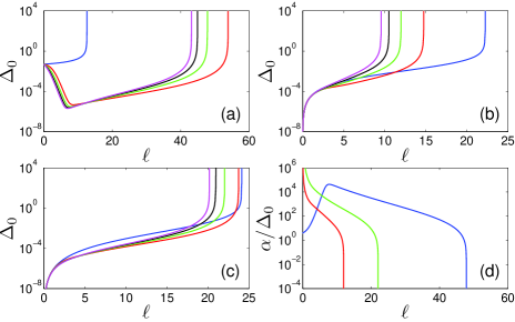
Figure 1: Flow of $\Delta_{0}$ caused by the interplay of RSP and Coulomb interaction in double-WSM, where $\Delta_{00}=0.05$ in (a), $\Delta_{10}=0.05$ in (b), and $\Delta_{30}=0.05$ in (c). In (a)-(c), the blue, red, green, black, and magenta curves represent the initial values $\alpha_{0}=0,0.1,0.2,0.3,0.4$, respectively. Dependence of the ratio $\alpha_{0}/\Delta_{0}$ on $\ell$ is shown in (d) with $\alpha_{0}=0.2$, where the blue, red, and green curves represent the values of $\Delta_{00}=0.05$, $\Delta_{10}=0.05$, $\Delta_{30}=0.05$, respectively. An initial value $\zeta_{0}^{d}=0.1$ is taken.

The stable fixed point of triple-WSM induced by the $x$-RVP exhibit similar behavior to the NFLs. In a loose sense, this state could be called a NFL Fu17 ; Roy16B ; Roy16C ; Pixley16A . However, we should remember that, strictly speaking, the coupling between fermions and static disorder $x$-RVP is rather different from inelastic scattering. To reflect this difference, it might be more appropriate to use a different terminology. Here, we would consider the NFL-like behavior characterized by Eq. (26) and Eqs. (28)-(31) as stable critical behavior.

When $y$-RVP exists alone in the system, there is also a stable infrared fixed point, at which the quantum critical behavior is analogous to that caused by $x$-RVP. Thus, we will not further discuss the physical effects of $y$-RVP.

If the system contains only $z$-RVP, the RG equation for its strength parameter is given by

$$\frac{d\Delta_{3}}{d\ell}=\frac{1}{3}\Delta_{3}+\frac{1}{12}\Delta_{3}^{2}.$$ (32)

The corresponding solution has the form

$$\Delta_{3}=\frac{4e^{\frac{1}{3}\ell}\Delta_{30}}{\Delta_{30}+4-e^{\frac{1}{3}\ell}\Delta_{30}}.$$ (33)

It is clear that $\Delta_{3}$ flows to infinity at some finite energy scale if $\Delta_{30}$ takes any finite value. Therefore, the $z$-RVP is similar to RSP, and an arbitrarily weak $z$-RVP is able to drive a transition to CDM phase.

The above results inform us that the disorder effects on double- and triple-WSMs are very different: disorder always drives a CDM state of double-WSM, but can induce either CDM state or stable critical state, depending on the specific type of disorder. To better understand the difference, we list the asymptotic behavior of DOS and specific heat in different phases of double- and triple-WSMs in Tables 2 and 3, respectively.

Figure 2: (a)-(c): Flow of $\Delta_{0}$, $\alpha$, and $\alpha/\Delta_{0}$ due to interplay of RSP and Coulomb interaction in triple-WSM at a given value $\Delta_{00}=0.05$. Blue, red, green, black, and magenta curves represent the initial values $\alpha_{0}=0,0.003,0.005,0.01,0.015$, respectively. (d) shows the flowing diagram on the $\Delta_{0}$-$\alpha$ plane. Here, we assume that $\zeta_{0}^{t}=0.1$.

III.2 Interplay between interaction and disorder

We now consider the influence of the interplay between Coulomb interaction and disorder.

For double-WSM, we present the flow of $\Delta_{0}$ with $\Delta_{00}=0.05$ and $\Delta_{10}=\Delta_{20}=\Delta_{30}=0$ in Fig. 1(a). In the presence of Coulomb interaction, $\Delta_{0}$ first decreases with increasing $\ell$, but then starts to increase once $\ell$ exceeds certain threshold. As $\ell$ continues to grow, $\Delta_{0}$ finally flows to strong coupling regime at some finite energy scale. In Fig. 1(b) and Fig. 1(c), we show the curves of $\Delta_{0}$ obtained by assuming that the system contains, apart from Coulomb interaction, only $x$-RVP and only $z$-RVP, with initial values $\Delta_{10}=0.05$ and $\Delta_{30}=0.05$, respectively. An interesting result is that $\Delta_{0}$ is always dynamically generated and flows to strong coupling at sufficiently large $\ell$.

According to Figs. 1(a)-(c), irrespective of the initial value of Coulomb interaction strength, $\Delta_{0}$ always flows to strong coupling if any type of disorder has a finite strength. It is found that $\alpha$ also goes to the strong coupling regime, which is not depicted in Fig. 1, but the ratio $\alpha/\Delta_{0}\rightarrow 0$ in any case, as clearly shown in Fig. 1(d). This indicates that disorder is always more important than Coulomb interaction, and the low-energy properties of the system are mainly determined by the disorder, rather than by the Coulomb interaction. It was also found that RSP dominates over any component of RVP. An immediate conclusion is that double-WSM is always in the CDM phase, no matter the Coulomb interaction is incorporated or not. This is similar to the case of the 3D quadratical SM, which is found by Nandkishore et al. Nandkishore17 to be always in the CDM phase when Coulomb interaction and disorder are simultaneously present.

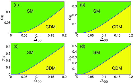
Figure 3: Phase diagrams of the triple-WSM in the presence of RSP and Coulomb interaction, plotted on the plane spanned by $\Delta_{00}$ and $\alpha_{0}$. The value of $\zeta_{0}^{t}$ is taken to be $0.1$, $0.5$, $1$, and $2$ in (a), (b), (c), and (d), respectively. There is always a critical line that separates the SM and CDM phases.

For triple-WSM, we show in Figs. 2(a)-(c) the flows of parameters $\Delta_{0}$, $\alpha$, and $\alpha/\Delta_{0}$ obtained by considering both RSP and Coulomb interaction. Fig. 2(d) presents the flow diagram of the two parameters $\Delta_{0}$ and $\alpha$. We find that, for weak Coulomb interaction, $\Delta_{0}$ and $\alpha$ still flow to strong couplings at some finite scale, but the ratio $\alpha/\Delta_{0}\rightarrow 0$, implying the dominance of RSP at low energies. However, if $\alpha_{0}$ is greater than a critical value, whose precise value is determined by $\Delta_{00}$, the parameters $\Delta_{0}$, $\alpha$, and also $\Delta_{0}/\alpha$ flow to zero at lowest energy limit. Apparently, the triple-WSM recovers a SM phase with vanishing $\rho(0)$ when the initial value of Coulomb interaction becomes sufficiently strong. In short, RSP is much more important than the weak Coulomb interaction, driving the system to become CDM, but the strong Coulomb interaction plays an overwhelming role than RSP and guarantees the stability of the SM phase. We notice that such behavior is very similar to that of 2D DSM caused by the interplay between the RSP and Coulomb interaction Ye99 ; Stauber05 ; WangLiu14 .

The phase diagram of triple-WSM in the plane of $\Delta_{00}$ and $\alpha_{0}$ is shown in Fig. 3. Obviously, there is a critical line, at which a QPT takes place between the SM and CDM phases. In the Figs. 3(a)-(d), $\zeta_{0}$ is taken $0.1$, $0.5$, $1$, and $2$ respectively. We can find that the change of $\zeta_{0}$ does not change the qualitative characteristic of the phase diagram, but quantitatively modify the critical line between SM and CDM phase. For ordinary WSMs, Goswami et al. Goswami11 showed that there is also an analogous critical line between the SM and CDM phases in the plane spanned by the initial strength parameters of Coulomb interaction and RSP. However, the crossover point of the critical line and axes is $(0,0)$ for triple-WSM, but $(\Delta_{00}^{c},0)$ for ordinary WSM, where $\Delta_{00}^{c}$ is a finite value. This feature arises from the fact that an arbitrarily weak RSP drives the triple-WSM to enter into a CDM phase if there is only RSP. The situation is different in the usual WSM, where only a sufficiently strong RSP can drive a CDM transition Goswami11 .

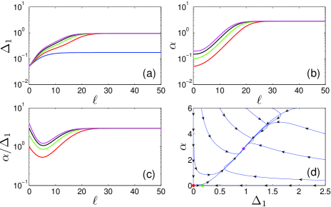
Figure 4: (a)-(c): Flow of $\Delta_{1}$, $\alpha$, and $\alpha/\Delta_{1}$ caused by the interplay of $x$-RVP and Coulomb interaction in triple-WSM at a given value $\Delta_{10}=0.05$. Blue, red, green, black, and magenta curves correspond to $\alpha_{0}=0,0.05,0.1,0.15,0.2$, respectively. Flowing diagram on the $\Delta_{1}$-$\alpha$ plane is shown in (d). Here, we choose an initial value $\zeta_{0}^{t}=0.1$.

We then consider the mutual influence of $x$-RVP and Coulomb interaction. According to Fig. 4, $\Delta_{1}$ and $\alpha$ always flow to a stable infrared fixed point (${\Delta_{1n}^{*}},\alpha_{n}^{*}$). This stable fixed point is possibly characterized by the emergence of unusual critical behavior, which is physically distinct from both SM and CDM states. We emphasize that the existence and property of such a fixed point needs to be further explored, because $\Delta_{1n}^{*}$ is only slightly smaller than unity whereas $\alpha_{n}^{*}\approx 3$. At such a fixed point, the validity of perturbative RG calculations is actually questionable. We expect that other non-pertubative method, such as functional RG (fRG) Metzner12 ; Bauer15 ; Sharma16 ; SbierskifRG17 or Monte Carlo simulation Foulkes01 ; Gull11 ; Tupitsyn17 , could be employed to further study this problem. When there is an interplay of Coulomb interaction and $y$-RVP, the low-energy properties are very similar to the case of $x$-RVP, and thus will not be further discussed.

We finally consider the interplay of Coulomb interaction and $z$-RVP. The RG solutions for parameters $\Delta_{3}$, $\alpha$, and $\alpha/\Delta_{3}$ are depicted in Figs. 5(a)-(c). The schematic flowing diagram in the $\Delta_{3}-\alpha$ plane is plotted in Fig. 5(d). According to these results, we find that $\Delta_{3}$ and $\alpha$ both flow to the strong coupling regime, where $\alpha$ dominates over $\Delta_{3}$. Therefore, the Coulomb interaction plays a more important role than $z$-RVP at low energies. A possible interpretation of such behavior is that the system becomes an interaction-dominated Mott insulator. This is an important issue that deserves further theoretical investigation.

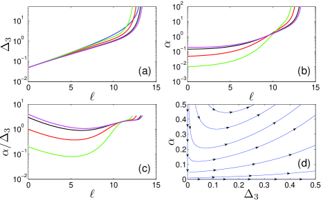
Figure 5: (a)-(c): Flow of $\Delta_{3}$, $\alpha$, and $\alpha/\Delta_{3}$ caused by the interplay of $z$-RVP and Coulomb interaction in triple-WSM. In (a)-(c), $\Delta_{30}=0.05$, and the blue, red, green, black, and magenta curves represent the initial values $\alpha_{0}=0,0.05,0.1,0.15,0.2$, respectively. (d) shows the flowing diagram in the $\Delta_{3}$-$\alpha$ plane. An initial value $\zeta_{0}^{t}=0.1$ is taken.

For triple-WSM, if two types of disorder are initially considered, other types of disorder are always generated, and all the disorder parameters flow to infinity at finite energy scale. The running behavior of $\Delta_{0}$ by considering the coexistence of two types of disorder is presented in Fig. 6, which clearly shows that $\Delta_{0}$ always flows to the strong coupling regime. The strength of Coulomb interaction $\alpha$ also flows to infinity at the same energy scale. However, the ratios $\Delta_{1}/\Delta_{0}$, $\Delta_{2}/\Delta_{0}$, $\Delta_{3}/\Delta_{0}$ and $\alpha/\Delta_{0}$ all decrease down to zero. From Fig. 7, obtained under the same initial conditions as Fig. 6, we observe that both $\Delta_{1}/\Delta_{0}$ or $\Delta_{3}/\Delta_{0}$ vanish at finite $\ell$. Therefore, the low-energy physics is dominated by RSP, and the system is inevitably turned into the CDM phase. This implies that triple-WSM always becomes a CDM if two or more types of disorder exist simultaneously, which is similar to double-WSM. It is interesting that similar phenomena occur in 2D DSM Evers08 ; Ostrovsky06 ; Foster12 ; JingWang17 , where RSP, RVP, and random mass can induce CDM transition, stable critical state, and logarithmic-like corrections to observable quantities, respectively. If any two types of disorder coexist in 2D DSM, the system always undergoes a CDM transition.

IV Further analysis of RG results

In this section, we present a further analysis of the RG results obtained and discussed in the last section.

IV.1 Difference between double- and triple-WSMs

An important indication of the analysis presented in Section III is that double- and triple-Weyl fermions manifest very different low-energy behavior in response to static short-range disorder. In the following, we explain the physical origin of such marked difference, and also compare with the usual WSM.

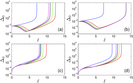
Figure 6: (a)-(c): Flow of $\Delta_{0}$ driven by two types of disorder and Coulomb interaction in triple-WSM. (a): $\Delta_{00}=0.01$, $\Delta_{10}=0.01$; (b): $\Delta_{00}=0.01$, $\Delta_{30}=0.01$; (c): $\Delta_{10}=0.01$, $\Delta_{20}=0.01$; (d): $\Delta_{10}=0.01$, $\Delta_{30}=0.01$. Blue, red, green, black, and magenta curves represent the initial values $\alpha_{0}=0,0.05,0.1,0.15,0.2$, respectively. Here, we set $\zeta_{0}^{t}=0.1$.

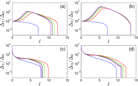
Figure 7: (a)-(d): Flow of $\Delta_{1}/\Delta_{0}$ in (a), (c), and $\Delta_{3}/\Delta_{0}$ in (b) and (d). The initial conditions are the same as Fig. 6.

The free propagators for the usual, double-, and triple-Weyl fermions are given by

$$G_{0}^{u}(\omega,\mathbf{k}) = \frac{1}{-i\omega+v\left(k_{x}\sigma_{1}+k_{y}\sigma_{2}+k_{z}\sigma_{3}\right)},$$

$$G_{0}^{d}(\omega,\mathbf{k}) = \frac{1}{-i\omega+Ad_{1}(\mathbf{k})\sigma_{1}+Ad_{2}(\mathbf{k})\sigma_{2}+vk_{z}\sigma_{3}},$$

$$G_{0}^{t}(\omega,\mathbf{k}) = \frac{1}{-i\omega+Bg_{1}(\mathbf{k})\sigma_{1}+Bg_{2}(\mathbf{k})\sigma_{2}+vk_{z}\sigma_{3}},$$

where $d_{1}(\mathbf{k})=k_{x}^{2}-k_{y}^{2}$, $d_{2}(\mathbf{k})=2k_{x}k_{y}$, $g_{1}(\mathbf{k})=k_{x}^{3}-3k_{x}k_{y}^{2}$, and $g_{2}(\mathbf{k})=k_{y}^{3}-3k_{y}k_{x}^{2}$. For usual WSM, the fermion propagator satisfies the relation

$$G_{0}^{u}(\omega,\mathbf{k})+G_{0}^{u}(-\omega,-\mathbf{k})=0.$$ (34)

It is easy to verify that the fermion propagator in double-WSM does not satisfy this relation, i.e.,

$$G_{0}^{d}(\omega,\mathbf{k})+G_{0}^{d}(-\omega,-\mathbf{k})\neq 0.$$ (35)

For triple-WSM, one finds that

$$G_{0}^{t}(\omega,\mathbf{k})+G_{0}^{t}(-\omega,-\mathbf{k})=0,$$ (36)

which shares the same property as usual WSM.

The diagrams for one-loop corrections to fermion-disorder vertex are given by Fig. 17 in the Appendix E. Amongst these diagrams, the sum of (b) and (c) are

$$V_{ij}^{u,d,t(2)+(3)} = 2\Delta_{i}\Delta_{j}\int^{\prime}\frac{d^{3}\mathbf{k}}{(2\pi)^{3}}\left(\psi_{a}^{{\dagger}}\Gamma_{i}G_{0}^{u,d,t}(0,\mathbf{k})\Gamma_{j}\psi_{a}\right)$$ (37)

$$\times\left\{\psi_{b}^{{\dagger}}\left[\Gamma_{j}G_{0}^{u,d,t}(0,\mathbf{k})\Gamma_{i}\right.\right.$$

$$\left.\left.+\Gamma_{i}G_{0}^{u,d,t}(0,-\mathbf{k})\Gamma_{j}\right]\psi_{b}\right\}.$$

In the case of usual WSM with $\Gamma_{i}=\Gamma_{j}$, the constraint of Eq. (34) ensures that the total contribution from these two Feynman diagrams vanishes, namely

$$V_{ii}^{u(2)+(3)}=0.$$ (38)

For double-WSM with $\Gamma_{i}=\Gamma_{j}$, we know from Eq. (35) that the total contribution

$$V_{ii}^{d(2)+(3)}\neq 0,$$ (39)

which differs from usual WSM. More concretely, we have

$$V_{00}^{(2)+(3)} = \frac{\Delta_{0}^{2}}{8\pi vA}\sum_{j=1,2}\left(\psi_{a}^{{\dagger}}\sigma_{j}\psi_{a}\right)\left(\psi_{b}^{{\dagger}}\sigma_{j}\psi_{b}\right)\ell,$$ (40)

$$V_{11}^{(2)+(3)} = \frac{\Delta_{1}^{2}}{8\pi vA}\sum_{j=1,2}\left(\psi_{a}^{{\dagger}}\sigma_{j}\psi_{a}\right)\left(\psi_{b}^{{\dagger}}\sigma_{j}\psi_{b}\right)\ell,$$ (41)

$$V_{22}^{(2)+(3)} = \frac{\Delta_{2}^{2}}{8\pi vA}\sum_{j=1,2}\left(\psi_{a}^{{\dagger}}\sigma_{j}\psi_{a}\right)\left(\psi_{b}^{{\dagger}}\sigma_{j}\psi_{b}\right)\ell,$$ (42)

$$V_{33}^{(2)+(3)} = \frac{\Delta_{3}^{2}}{8\pi vA}\sum_{j=1,2}\left(\psi_{a}^{{\dagger}}\sigma_{j}\psi_{a}\right)\left(\psi_{b}^{{\dagger}}\sigma_{j}\psi_{b}\right)\ell.$$ (43)

The triple-WSM is very similar to the usual WSM, which means that, in the case $\Gamma_{i}=\Gamma_{j}$, the total contribution of Figs. 17(b) and (c) satisfies

$$V_{ii}^{t(2)+(3)}=0,$$ (44)

as a direct results of Eq. (36).

The close analogy between usual and triple-WSMs, reflected in the constraints given by Eqs. (38) and (44), leads to common properties shared by these two systems. For instance, one type of disorder can exist individually in usual and triple-WSMs. However, this is not possible in a double-WSM. Due to the non-zero contributions shown in Eqs. (40)-(43), one type of disorder cannot exist individually because it dynamically generates other types of disorder BeraRoy16 . We have pointed out such special property of double-WSM in Section III. From the above analysis, we can now conclude that the specific disorder scattering processes represented by Figs. 17(b) and (c) are suppressed in both the usual and triple-WSMs, where the Hamiltonian $\mathcal{H}(\mathbf{k})$ becomes $-\mathcal{H}(\mathbf{k})$ under the transformation $\mathbf{k}\rightarrow-\mathbf{k}$, but make non-trivial contributions in the case of double-WSM.

While the disorder effects on the usual and triple-WSMs are similar in some aspects, they are definitely not identical. In a usual WSM containing only one component of RVP, Sbierski et al. Sbierski16 showed that the disorder strength parameter satisfies the equation

$$\frac{d\Delta_{i}}{d\ell}=-\Delta_{i}-C\Delta_{i}^{2},$$ (45)

where $i=1$, $2$, or $3$, and $C$ is a positive constant. For the triple-WSM with only $x$- or $y$-component of RVP, we have showed in Sec. III that the RG equation is

$$\frac{d\Delta_{i}}{d\ell}=\frac{1}{3}\Delta_{i}-\frac{23}{12}\Delta_{i}^{2},$$ (46)

where $i=1$ or $2$. The second terms of the right hand sides of Eq. (45) and Eq. (46), representing the one-loop correction to beta function, are both negative, which is valid if the system contains only one component of RVP and the relations given by Eq. (34) and Eq. (36) are satisfied. However, the first terms, determined by the scaling dimension at tree-level, are opposite in sign. This difference is owing to the fact that the usual Weyl and triple-Weyl fermions have different dispersions. According to Eq. (45), we know that the disorder strength for one component of RVP always flows to zero at low energies in the usual WSM Sbierski16 . If triple-WSM containing only $x$- or $y$-component of RVP, there is a stable fixed point $\Delta_{i}^{*}=\frac{4}{23}$, which is obtained from Eq. (46).

For double-WSM, the situation is in sharp contrast to the usual and triple-WSMs. As demonstrated in the last section, the double-WSM is always driven by $x$-RVP (or $y$-RVP) to enter into a CDM phase. This result should be attributed to Eq. (35).

IV.2 Stability of the infrared fixed point of triple-WSM

In Section III, we have found a stable infrared fixed point in our one-loop RG analysis of the triple-WSM containing only the $x$- or $y$-component of RVP. A natural question arises as whether such a fixed point survives the higher order corrections. To address this issue, we now discuss whether the one-loop results are still valid after including two-loop corrections.

It is useful to first briefly review the recent progress of disorder effects in 3D DSM/WSM. For 3D DSM and WSM, one-loop RG studies Goswami11 ; Roy14 ; Syzranov15A ; Syzranov15B revealed that weak RSP is irrelevant, but becomes relevant if the RSP strength is beyond a critical value, which then drives a SM-CDM transition. To the one-loop order, the dynamical critical exponent at quantum critical point (QCP) from SM to CDM is $z=\frac{3}{2}$, and the correlation length exponent is $\nu=1$ Goswami11 ; Roy14 ; Syzranov15A ; Syzranov15B . Two-loop order corrections were also calculated by various approaches, including replica method Roy14 ; Roy16Erratum , supersymmetry technique Syzranov16A , correspondence with Gross-Neveu model Roy16Erratum , and correspondence with Gross-Neveu-Yukawa model Louvet16 . These studies confirmed that there is still a quantum phase transition (QPT) from SM to CDM, which implies that the conclusion obtained by one-loop RG analysis is qualitatively robust against higher order corrections. Quantitatively, the critical disorder strength, dynamical critical exponent $z$, and correlation length exponent $\nu$ are more or less modified after including two-loop corrections. Syzranov et al. Syzranov16A found $z\approx 1.4$ and $\nu\approx 0.67$ after making two-loop calculations. Roy and Das Sarma Roy16Erratum also reported that $\nu\approx 0.67$ up to two-loop order. Louvet et al. Louvet16 got a nearly identical value $\nu\approx 0.65-0.67$ in their two-loop calculations. The same problem has also been investigated by using the numerical simulation method BeraRoy16 ; Kobayashi14 ; Liu16 ; Pixley16A ; Roy16B ; Sbierski14 ; Sbierski15 ; Fu17 , where it is found that a SM-CDM transition always occurs, providing further support to the conclusion reached by the one-loop RG analysis. Moreover, some numerical studies Pixley16B ; Pixley16C ; Pixley17 suggested that the rare region effect can induce exponentially small zero-energy DOS $\rho(0)$ in the case of weak disorder, which broadens the QCP to a quantum critical region at finite energy-scale. Actually, the dynamical critical exponent $z$ obtained by most of the existing numerical studies BeraRoy16 ; Kobayashi14 ; Sbierski15 ; Liu16 ; Pixley16A ; Roy16B ; Fu17 is well consistent with the one-loop RG result $z=\frac{3}{2}$. Although the precise value of $\nu$ is still controversial BeraRoy16 ; Kobayashi14 ; Liu16 ; Pixley16A ; Roy16B ; Sbierski15 ; Fu17 , the existing extensive analytical and numerical works suggest that one-loop RG results are at least qualitatively reliable.

In a recent work, Sbierski et al. Sbierski16 studied the impact of RVP on 3D WSM by making a one-loop RG analysis along with numerical simulation. Their one-loop RG result is that 3D WSM is always in the SM phase if the system contains only one component of RVP, and their numerical simulations found that 3D WSM stays in the SM phase even if RVP becomes very strong, which is well consistent with the one-loop RG result.

In the case of triple-WSM, the strong anisotropy in the fermion dispersion makes it very difficult to carry out an analytical calculation of two-loop corrections to the RG equations. We would like to leave this for future study. To estimate the possible impact of two-loop contributions on the one-loop conclusion, we now present a generic analysis. After including two-loop corrections, the RG equation could be formally written as

$$\frac{d\Delta_{i}}{d\ell}=\frac{1}{3}\Delta_{i}-\frac{23}{12}\Delta_{i}^{2}+C_{2\mathrm{LP}}\Delta_{i}^{3},$$ (47)

where $i=1$ or $i=2$. The first and second terms on the right hand side of Eq. (47) represent the tree-level and one-loop contributions, respectively, whereas the third term represents the two-loop contribution, where $C_{2\mathrm{LP}}$ is a constant. We assume that $C_{2\mathrm{LP}}$ can take all possible values, and examine under what circumstances the stable fixed point obtained in our one-loop analysis is robust.

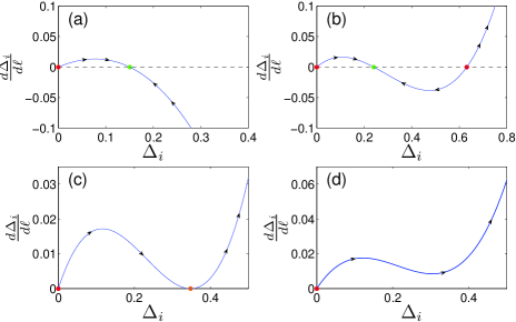
Figure 8: Dependence of $\frac{d\Delta_{i}}{d\ell}$ on $\Delta_{i}$ with $i=1$ or $2$ in four different cases. (a) $C_{2\mathrm{LP}}<0$; (b) $0<C_{2\mathrm{LP}}<\frac{529}{192}$; (c) $C_{2\mathrm{LP}}=\frac{529}{192}$; (d) $C_{2\mathrm{LP}}>\frac{529}{192}$. We assume $C_{2\mathrm{LP}}=-2,2.2,3$ in (a), (b), and (d), respectively. The red and green points represent unstable and stable fixed point, respectively. The orange point in (c) is stable from the left side, but is unstable from the right side.

There are four different cases. If $C_{2\mathrm{LP}}<0$, there is always a stable fixed point

$$\Delta_{i}^{*}=\frac{\frac{23}{12}-\sqrt{\left(\frac{23}{12}\right)^{2}-\frac{4}{3}C_{2\mathrm{LP}}}}{2C_{2\mathrm{LP}}},$$ (48)

which is shown in Fig. 8(a). If $0<C_{2\mathrm{LP}}<\frac{529}{192}$, as depicted in Fig. 8(b), there exists a stable fixed point

$$\Delta_{i}^{s*}=\frac{\frac{23}{12}-\sqrt{\left(\frac{23}{12}\right)^{2}-\frac{4}{3}C_{2\mathrm{LP}}}}{2C_{2\mathrm{LP}}},$$ (49)

and also a finite unstable fixed point

$$\Delta_{i}^{us*}=\frac{\frac{23}{12}+\sqrt{\left(\frac{23}{12}\right)^{2}-\frac{4}{3}C_{2\mathrm{LP}}}}{2C_{2\mathrm{LP}}}.$$ (50)

When $C_{2\mathrm{LP}}=\frac{529}{192}$, the above two fixed points merge to one single fixed point

$$\Delta_{i}^{*}=\frac{8}{23},$$ (51)

which is displayed in Fig. 8(c).

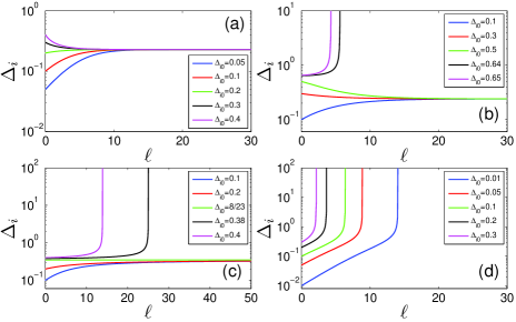
Figure 9: Dependence of $\Delta_{i}$ with $i=1$ or $2$ on $\ell$ in four different cases. We assume $C_{2\mathrm{LP}}=-2,2.2,\frac{529}{192},3$ in (a)-(d), respectively.

If the initial disorder strength $\Delta_{i0}$ is below this critical value, i.e., $0<\Delta_{i0}<\Delta_{i}^{*}$, it always flows to this fixed point in the lowest energy limit. However, if $\Delta_{i0}>\Delta_{i}^{*}$, the disorder strength parameter flows away, which turns the triple-WSM into a CDM. We finally consider the case of $C_{2\mathrm{LP}}>\frac{529}{192}$. As shown in Fig. 8(d), there is only one unstable fixed point $\Delta_{i}^{*}=0$. In this case, the stable infrared fixed point obtained in the one-loop RG analysis is eliminated by the two-loop corrections, and even arbitrarity weak disorder drives a CDM transition. The flows of disorder strength in triple-WSM that contains only one component of RVP is presented in Fig. 9 for four representative values of $C_{2\mathrm{LP}}$. From Figs. 8 and 9, we can see that there is always a stable infrared fixed point for $C_{2\mathrm{LP}}<\frac{529}{192}$. The concrete value of $C_{2\mathrm{LP}}$ will be calculated in the future. We expect that numerical techniques, such as kernel polynomial method BeraRoy16 ; Kobayashi14 ; Liu16 ; Pixley16A ; Sbierski16 and Lanczos method Fu17 would be employed to determine whether the stable infrared fixed point revealed in our one-loop RG calculation survives higher order corrections.

IV.3 Influence of Coulomb impurity on triple-WSM

Apart from short-range disorder, there might be disorder with long-range correlation in various SMs Fedorenko12 ; DasSarma11 ; Nomura07 ; Khveshchenko07 ; Louvet17 ; Skinner14 ; Ominato15 . The most frequently encountered is Coulomb impurity, which is defined in a similar way to that of RSP, but is spatially long-ranged. Generically, the role played by long-range disorder is more important than short-range disorder in SMs. For 3D DSM/WSM, the physical effects of short-range disorder and long-range disorder turn out to be quite different. Weak short-range RSP is irrelevant and becomes relevant if its strength is large enough. Recent RG analysis of Louvet et al. Louvet17 found that an arbitrarily weak long-range disorder drives the 3D WSM to become a CDM if such disorder decays more slowly than $1/r^{2}$ for large $r$. It is thus clear that arbitrarily weak Coulomb impurity, which decays as $1/r$, can lead to a SM-CDM transition. Similar conclusion was found to be applicable to 3D DSM Skinner14 ; Ominato15 .

Since the present work is focused on the interplay between the long-range Coulomb interaction and short-range disorder, we will not present a thorough analysis of the physical effects of long-range disorder. Here, we will only consider a special case, namely the influence of Coulomb impurity on the low-energy properties of triple-WSM. The extension to double-WSM and other types of long-range disorder would be straightforward.

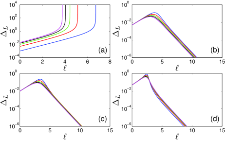
Figure 10: Flow of the Coulomb impurity parameter $\Delta_{L}$ in triple-WSM. In (a), there is only Coulomb impurity, and blue, red, green, black, and magenta curves represent the initial values $\Delta_{L0}=0.001,0.005,0.01,0.015,0.02$, respectively. In (b)-(d), Coulomb interaction and Coulomb impurity are both present. $\Delta_{L0}=0.005$, $0.01$, and $0.05$ is taken in (b), (c), and (d), where blue, red, green, black, and magenta curves are obtained at $\alpha_{0}=0.005,0.01,0.015,0.02,0.025$, respectively. Here, we set $\zeta_{0}^{t}=0.1$.

Using the replica method, one can write down the following action for triple-Weyl fermions embedded in the potential generated by Coulomb impurity

$$S_{\mathrm{Coim}} = \frac{\Delta_{L}}{2}\int\frac{d\omega_{1}d\omega_{2}d^{3}\mathbf{k}_{1}d^{3}\mathbf{k}_{2}d^{3}\mathbf{k}_{3}}{(2\pi)^{8}}$$ (52)

$$\times\frac{g^{2}}{|\mathbf{k}_{1}+\mathbf{k}_{2}|_{\bot}^{2}+\eta\left(k_{1z}+k_{2z}\right)^{2}}$$

$$\times\Psi^{\dagger}_{a}(i\omega_{1},\mathbf{k}_{1})\mathbbm{1}\Psi_{a}(i\omega_{1},\mathbf{k}_{2})\Psi_{b}^{\dagger}(i\omega_{2},\mathbf{k}_{3})\mathbbm{1}$$

$$\times\Psi_{b}(i\omega_{2},-\mathbf{k}_{1}-\mathbf{k}_{2}-\mathbf{k}_{3}),$$

where $\Delta_{L}$ is introduced to quantify the strength of Coulomb impurity, and $g^{2}=4\pi e^{2}/\epsilon$ and $\eta$ are defined in the same way as in Sec. II.

To make our analysis more generic, we will consider the interplay of Coulomb interaction, Coulomb impurity, and short-range RSP. The coupled RG equations are

$$\frac{dZ_{f}}{d\ell} = -\left(\frac{5}{4}\Delta_{0}+C_{L1}\Delta_{L}\right)Z_{f},$$ (53)

$$\frac{dB}{d\ell} = \left(C_{2}^{t}-\frac{5}{4}\Delta_{0}-C_{L1}\Delta_{L}+C_{L2}\Delta_{L}\right)B,$$ (54)

$$\frac{dv}{d\ell} = \left(C_{3}^{t}-\frac{5}{4}\Delta_{0}-C_{L1}\Delta_{L}+C_{L3}\Delta_{L}\right)v,$$ (55)

$$\frac{d\alpha}{d\ell} = \Big{(}-C_{\bot}^{t}-C_{3}^{t}+\frac{5}{4}\Delta_{0}$$ (56)

$$+C_{L1}\Delta_{L}-C_{L3}\Delta_{L}\Big{)}\alpha,$$

$$\frac{d\beta^{t}}{d\ell} = \left(\frac{4}{3}-\frac{2}{3}C_{2}^{t}+C_{3}^{t}-\frac{5}{12}\Delta_{0}-\frac{1}{3}C_{L1}\Delta_{L}\right.$$ (57)

$$\left.-\frac{2}{3}C_{L2}\Delta_{L}+C_{L3}\Delta_{L}-\beta^{t}\right)\beta^{t},$$

$$\frac{d\eta}{d\ell} = \left(-\frac{4}{3}-C_{\bot}^{t}+\beta^{t}\right)\eta,$$ (58)

$$\frac{d\Delta_{0}}{d\ell} = \frac{1}{3}\Delta_{0}-\left(\frac{2}{3}C_{2}^{t}+C_{3}^{t}+2C_{\bot}^{t}+2\beta^{t}\right)\Delta_{0}$$ (59)

$$+\left(\frac{5}{3}C_{L1}-\frac{2}{3}C_{L2}-C_{L3}\right)\Delta_{0}\Delta_{L}$$

$$+\frac{25}{12}\Delta_{0}^{2},$$

$$\frac{d\Delta_{L}}{d\ell} = \Delta_{L}-\left(C_{3}^{t}+3C_{\bot}^{t}+2\beta^{t}\right)\Delta_{L}+\frac{5}{4}\Delta_{0}\Delta_{L}$$ (60)

$$+\left(C_{L1}-C_{L3}\right)\Delta_{L}^{2}.$$

The parameter $\Delta_{L}$ has been redefined as follows:

$$\frac{c_{f}\Delta_{L}g^{2}}{v\Lambda}\rightarrow\Delta_{L}.$$ (61)

The concrete expressions for $C_{Li}\equiv C_{Li}(\zeta^{t})$, where $i=1,2,3$ and $\zeta^{t}=\frac{\eta B^{\frac{2}{3}}\Lambda^{\frac{4}{3}}}{v^{2}}$, are presented in Appendix G.

If there is only Coulomb impurity, the dependence of $\Delta_{L}$ on $\ell$ is displayed in Fig. 10(a). The parameter $\Delta_{L}$ always flows to the strong coupling regime, thus the Coulomb impurity always leads to a CDM phase. When both Coulomb impurity and long-range Coulomb interaction are considered, the parameter $\Delta_{L}$ exhibits distinct behavior. As can be seen from Figs. 10(b)-(d), $\Delta_{L}$ flows to zero rapidly at low energies. Thus, the SM phase is restored due to long-range Coulomb interaction, and the Coulomb impurity becomes relatively unimportant. This behavior is presumably caused by the special anisotropic screening effect induced by Coulomb interaction.

We then neglect the Coulomb interaction and analyze the interplay between Coulomb impurity and short-range RSP. The RG equations for $\Delta_{0}$ and $\Delta_{L}$ are

$$\frac{d\Delta_{0}}{d\ell} = \left[\frac{1}{3}+\left(\frac{5}{3}C_{L1}-\frac{2}{3}C_{L2}-C_{L3}\right)\Delta_{L}\right.$$ (62)

$$\left.+\frac{25}{12}\Delta_{0}\right]\Delta_{0},$$

$$\frac{d\Delta_{L}}{d\ell} = \left[1+\frac{5}{4}\Delta_{0}+\left(C_{L1}-C_{L3}\right)\Delta_{L}\right]\Delta_{L}.$$ (63)

In this case, the RG flows of $\Delta_{0}$, $\Delta_{L}$, and $\Delta_{0}/\Delta_{L}$ are presented in Figs. 11(a)-(c) respectively. We observe that $\Delta_{0}$, $\Delta_{L}$, and $\Delta_{0}/\Delta_{L}$ all formally diverge at some finite energy scale. Thus, RSP dominates over Coulomb impurity. The parameter $\zeta^{t}$ also flows to infinity simultaneously at finite energy scale, as shown in Fig. 10(d).

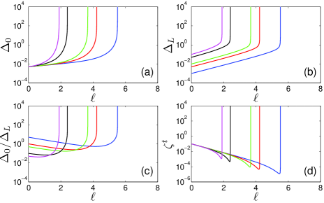
Figure 11: Flow of $\Delta_{0}$ in (a), $\Delta_{L}$ in (b), $\Delta_{0}/\Delta_{L}$ in (c), and $\zeta^{t}$ in (d). Both RSP and Coulomb impurity are considered, but Coulomb interaction is ignored. $\Delta_{00}=0.005$ is taken, and blue, red, green, black, and magenta curves represent the initial values $\Delta_{L0}=0.001,0.005,0.01,0.05,0.1$, respectively. Here, we choose an initial value $\zeta_{0}^{t}=0.1$.

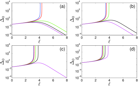
Figure 12: Flow of $\Delta_{0}$ caused by the interplay of RSP, Coulomb impurity, and Coulomb interaction in triple-WSM. Blue, red, green, black, and magenta curves represent the initial values $\alpha_{0}=0.003,0.005,0.01,0.015,0.02$, respectively. $\Delta_{L0}$ is taken as $0.001$, $0.004$, $0.007$, and $0.01$ in (a), (b), (c), and (d) respectively. An initial value $\zeta_{0}^{t}=0.1$ is chosen.

To understand these results, we now analyze the running behavior of the ratio $\Delta_{L}/\Delta_{0}$. The RG equation is

$$\frac{d(\Delta_{L}/\Delta_{0})}{d\ell}=\left(\frac{2}{3}-\frac{10}{12}\Delta_{0}-\frac{2}{3}C_{L1}+\frac{2}{3}C_{L2}\right)\frac{\Delta_{L}}{\Delta_{0}}.$$ (64)

The first term in the parenthesis, namely $\frac{2}{3}$, tells us that Coulomb impurity dominates over RSP at the tree-level. The second term is negative, and formally diverges as $\Delta_{0}$ flows to infinity. The contribution $\frac{2}{3}(C_{L2}-C_{L1})$ decreases with growing $\zeta^{t}$. It is easy to verify that the summation of all the terms in the parenthesis goes to negative infinity, which implies that the ratio $\Delta_{L}/\Delta_{0}$ eventually flows to zero. This explains why RSP becomes more important than the Coulomb impurity at low energies. The apparently anisotropic dispersion of triple-Weyl fermions is likely responsible for this property.

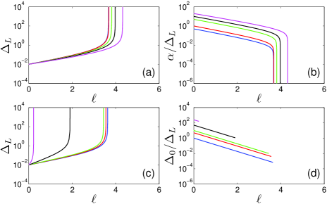
Figure 13: RG results for usual WSM. Coulomb impurity and Coulomb interaction are both included in (a) and (b) with $\Delta_{L0}=0.01$, where blue, red, green, black, and magenta curves stand for $\alpha_{0}=0.005,0.01,0.05,0.1,0.2$, respectively. Coulomb impurity and RSP are both considered in (c) and (d) with $\Delta_{L0}=0.01$, where blue, red, green, black, and magenta curves represent $\Delta_{0}=0.01,0.05,0.1,0.5,2.2$, respectively.

For triple-WSM that contains RSP, Coulomb impurity, and Coulomb interaction, the $\ell$-dependence of $\Delta_{0}$ is shown in Fig. 12. We observe that, for different initial conditions, $\Delta_{0}$ either vanishes or flows to infinity, which indicates that triple-WSM could be in the SM or CDM phase. Comparing the results presented in Fig. 12, one finds that increasing the strength of Coulomb impurity promotes CDM transition. If the strength parameters for RSP and Coulomb impurity are fixed, the SM phase can be restored by strong Coulomb interaction.

We now consider the impact of Coulomb impurity in the usual WSM, which will be compared with the case of triple-WSM. In the presence of Coulomb interaction, Coulomb impurity, and RSP, the RG equations for the corresponding parameters are given by

$$\frac{dZ_{f}}{d\ell} = -\left(\Delta_{0}+\Delta_{L}\right)Z_{f},$$ (65)

$$\frac{dv}{d\ell} = \left(\frac{2\alpha}{3\pi}-\Delta_{0}-\frac{4}{3}\Delta_{L}\right)v,$$ (66)

$$\frac{d\alpha}{d\ell} = \alpha\left(\Delta_{0}+\frac{4}{3}\Delta_{L}-\frac{4}{3\pi}\alpha\right),$$ (67)

$$\frac{d\Delta_{0}}{d\ell} = \left(-1+2\Delta_{0}+\frac{8}{3}\Delta_{L}-\frac{8}{3\pi}\alpha\right)\Delta_{0},$$ (68)

$$\frac{d\Delta_{L}}{d\ell} = \left(1+\frac{8}{3}\Delta_{L}+2\Delta_{0}-\frac{10}{3\pi}\alpha\right)\Delta_{L},$$ (69)

where we have made the replacements:

$$\frac{\Delta_{0}\Lambda}{2\pi^{2}v^{2}}\rightarrow\Delta_{0},\quad\frac{\Delta_{L}g^{2}}{2\pi^{2}v^{2}\Lambda}\rightarrow\Delta_{L}.$$ (70)

We present in in Fig. 13(a) the results obtained when there are Coulomb impurity and Coulomb interaction. We find that $\Delta_{L}$ exhibits runaway behavior, and that $\alpha$ also flows to strong coupling. However, the ratio $\alpha/\Delta_{L}$ vanishes rapidly with growing $\ell$, as clearly shown in Fig. 13(b). Therefore, the usual WSM undergoes a CDM phase transition driven by Coulomb impurity.

We then assume that Coulomb impurity and RSP exist simultaneously, but the long-range Coulomb interaction is neglected. The RG equations for $\Delta_{0}$ and $\Delta_{L}$ are

$$\frac{d\Delta_{0}}{d\ell} = \left(-1+2\Delta_{0}+\frac{8}{3}\Delta_{L}\right)\Delta_{0},$$ (71)

$$\frac{d\Delta_{L}}{d\ell} = \left(1+\frac{8}{3}\Delta_{L}+2\Delta_{0}\right)\Delta_{L}.$$ (72)

As shown in Fig. 13(c), $\Delta_{L}$ always approaches to infinity at some finite energy scale. $\Delta_{0}$ also flows to strong coupling at the same energy scale. As depicted in Fig. 13(d), $\Delta_{0}/\Delta_{L}$ deceases monotonously with growing of $\ell$. If the initial value $\Delta_{00}/\Delta_{L0}$ is very large, $\Delta_{0}/\Delta_{L}$ still takes a large value at the finite energy scale, in which $\Delta_{0}$ and $\Delta_{L}$ become divergent. If the initial value $\Delta_{00}/\Delta_{L0}$ is not very large, $\Delta_{0}/\Delta_{L}$ takes a value smaller than unity finally. Form the Eqs. (71) and (72), we can get the RG equation for the ratio $\Delta_{L}/\Delta_{0}$

$$\frac{d(\Delta_{L}/\Delta_{0})}{d\ell}=2\frac{\Delta_{L}}{\Delta_{0}}.$$ (73)

It is clear that there is only tree-level contribution. The one-loop order corrections do not alter the behavior of $\Delta_{L}/\Delta_{0}$. If Coulomb impurity, RSP, and Coulomb interaction are all included, usual WSM is always turned into the CDM phase.

The above analysis show that the triple-WSM and usual WSM exhibit quite different behavior in response to the interplay of Coulomb impurity, RSP, and Coulomb interaction, which should be attributed to the difference in their fermion dispersions.

V Summary

In summary, we have systematically studied the low-energy behavior of double- and triple-WSMs induced by the interplay between long-range Coulomb interaction and disorder. After performing a detailed RG analysis, we have showed that such an interplay has distinct influences on the dynamics of double- and triple-Weyl fermions. The double-WSM is always in a CDM phase if the system contains any type of disorder, such as RSP or RVP, and this feature is not altered by the addition of Coulomb interaction. However, the low-energy behavior of triple-Weyl fermions depend crucially on the type and strength of disorder. In the non-interacting limit, either RSP or $z$-RVP leads to a CDM transition, and $x$-RVP or $y$-RVP results in a stable quantum critical state. The interplay of RSP and weak Coulomb interaction turns the triple-WSM into a CDM phase, but the interplay of RSP and strong Coulomb interaction renders the stability of SM state. When the triple-WSM contains both $x$-RVP, or $y$-RVP, and Coulomb interaction, the system always flows to a stable infrared fixed point. The stability of this fixed point against two-loop corrections is also discussed. However, this problem is only partly answered, and more elaborate RG calculations are required to completely solve the problem. Finally, the interplay of $z$-RVP and Coulomb interaction may drive a QPT between SM and Mott insulator. We have demonstrated in great detail that the marked difference between the low-energy properties of double- and triple-WSMs is owing to the distinct response of the Hamiltonian under the transformation $\mathbf{k}\rightarrow-\mathbf{k}$.

We have also considered the impact of long-range Coulomb impurity on the low-energy behavior of triple-WSM. After making a RG analysis of the complicated interplay of Coulomb impurity, Coulomb interaction, and RSP, we find that, while the Coulomb impurity always drives the system to become CDM, the Coulomb interaction can effectively suppress the role played by Coulomb impurity and protect the SM state.

The diverse phases and the transitions between them predicted by our RG analysis could be verified by performing angle-resolved photoemission spectroscopy (ARPES) Damascelli03 ; Hasan17 and transport measurements. Recent first-principle calculations suggested that HgCr₂Se₄ Fang12 and SrSi₂ Huang16 are two promising candidates of the double-WSM. In addition, special SM systems, in which the fermions exhibit a linear dependence on one momentum component and cubic dependence on other two components, were predicted to be realizable in Rb(MoTe)₃ and Tl(MoTe)₃ LiuZunger17 . It is also possible to prepare the multi-WSM materials by microwave experiments ChenChan16 ; ChangChan17 . We expect that our theoretical predictions would be verified in the aforementioned materials in the future.

Appendix A Propagators

We now present the propagators of double- and triple-Weyl fermions and bosonic field that is introduced to represent the long-range Coulomb interaction. The boson self-energy is calculated in Appendix B. We then give the fermion self-energy induced by Coulomb interaction and disorder scattering in Appendix C. In Appendix D, the corrections to the fermion-boson coupling are computed. The vertex corrections to the fermion-disorder couplings are calculated in Appendix E. The RG equations for the model parameters of double- and triple-WSMs are derived in Appendix F. The expressions of $C_{Li}$, which enter into the RG equations for Coulomb impurity, are shown in Appendix G.

The free propagator of double-Weyl fermions is Lai15 ; Jian15

$$G_{0}^{d}(\omega,\mathbf{k})=\frac{1}{-i\omega+Ad_{1}(\mathbf{k})\sigma_{1}+Ad_{2}(\mathbf{k})\sigma_{2}+vk_{z}\sigma_{3}},$$ (74)

where $d_{1}(\mathbf{k})=k_{x}^{2}-k_{y}^{2}$ and $d_{2}(\mathbf{k})=2k_{x}k_{y}$. The free propagator of triple-Weyl fermions can be written as Zhang16

$$G_{0}^{t}(\omega,\mathbf{k})=\frac{1}{-i\omega+Bg_{1}(\mathbf{k})\sigma_{1}+Bg_{2}(\mathbf{k})\sigma_{2}+vk_{z}\sigma_{3}},$$ (75)

where $g_{1}(\mathbf{k})=k_{x}^{3}-3k_{x}k_{y}^{2}$ and $g_{2}(\mathbf{k})=k_{y}^{3}-3k_{y}k_{x}^{2}$. The propagator of bosonic field $\phi$ reads

$$D_{0}(\Omega,\mathbf{q})=\frac{1}{q_{\bot}^{2}+\eta q_{z}^{2}}.$$ (76)

Figure 14: Self-energy of bosonic field. The solid line represents the free fermion propagator, and the wavy line represents the boson propagator that is equivalent to the Coulomb interaction function.

Appendix B Boson self-energy

As shown in Fig. 14, to the leading order of perturbative expansion, the self-energy of bosonic field $\phi$ is given by

$$\Pi^{d,t}(\Omega,\mathbf{q}) = -g^{2}\int\frac{d\omega}{2\pi}\int\frac{d^{3}\mathbf{k}}{(2\pi)^{3}}\mathrm{Tr}\left[G_{0}^{d,t}(\omega,\mathbf{k})\right.$$ (77)

$$\left.\times G_{0}^{d,t}\left(\omega+\Omega,\mathbf{k}+\mathbf{q}\right)\right].$$

B.1 Double-Weyl fermions

Substituting Eq. (74) into Eq. (77), and then taking the limit $\Omega=0$, we obtain

$$\Pi^{d}(0,\mathbf{q}) = 2g^{2}\int_{-\infty}^{+\infty}\frac{d\omega}{2\pi}\int^{\prime}\frac{d^{3}\mathbf{k}}{(2\pi)^{3}}$$ (78)

$$\times\frac{1}{\left(\omega^{2}+E_{\mathbf{k}}^{2}\right)\left(\omega^{2}+E_{\mathbf{k}+\mathbf{q}}^{2}\right)}\Big{\{}\omega^{2}$$

$$-A^{2}\left(k_{x}^{2}-k_{y}^{2}\right)\left[\left(k_{x}+q_{x}\right)^{2}-\left(k_{y}+q_{y}\right)^{2}\right]$$

$$-4A^{2}k_{x}k_{y}\left(k_{x}+q_{x}\right)\left(k_{y}+q_{y}\right)$$

$$-v^{2}k_{z}\left(k_{z}+q_{z}\right)\Big{\}},$$

where $E_{\mathbf{k}}=\sqrt{A^{2}k_{\bot}^{4}+v^{2}k_{z}^{2}}$. Expanding $q_{i}$ up to the quadratical order leads us to

$$\Pi^{d}(0,\mathbf{q}) \approx q_{\bot}^{2}\frac{g^{2}}{4\pi^{2}}\int^{\prime}dk_{\bot}d|k_{z}|k_{\bot}\left(\frac{2A^{2}k_{\bot}^{2}}{E_{\mathbf{k}}^{3}}-\frac{A^{4}k_{\bot}^{6}}{E_{\mathbf{k}}^{5}}\right)$$ (79)

$$+q_{z}^{2}\frac{g^{2}}{8\pi^{2}}\int^{\prime}dk_{\bot}d|k_{z}|k_{\bot}\frac{v^{2}A^{2}k_{\bot}^{4}}{E_{\mathbf{k}}^{5}}.$$

To proceed, we introduce two new variables

$$E=\sqrt{A^{2}k_{\bot}^{4}+v^{2}k_{z}^{2}},\qquad\delta=\frac{Ak_{\bot}^{2}}{v\left|k_{z}\right|},$$ (80)

and perform integrations over $E$ and $\delta$ within the ranges $b\Lambda<E<\Lambda$ with $b=e^{-\ell}$ and $0<\delta<\infty$, which leads to

$$\Pi^{d}(0,\mathbf{q})=q_{\bot}^{2}C_{\bot}^{d}\ell+q_{z}^{2}C_{z}^{d}\ell,$$ (81)

where

$$C_{\bot}^{d}=\frac{g^{2}}{6\pi^{2}v},\qquad C_{z}^{d}=\frac{g^{2}}{64\pi v}\frac{v^{2}}{A\Lambda}.$$ (82)

B.2 Triple-Weyl fermions

Substituting Eq. (75) into (77) and taking the limit $\Omega=0$, we find that the boson self-energy has the form

$$\Pi^{t}(0,\mathbf{q}) = 2g^{2}\int_{-\infty}^{+\infty}\frac{d\omega}{2\pi}\int^{\prime}\frac{d^{3}\mathbf{k}}{(2\pi)^{3}}$$ (83)

$$\times\frac{1}{\left(\omega^{2}+E_{\mathbf{k}}^{2}\right)\left(\omega^{2}+E_{\mathbf{k}+\mathbf{q}}^{2}\right)}\Big{\{}\omega^{2}$$

$$-B^{2}\left(k_{x}^{3}-3k_{x}k_{y}^{2}\right)\left[\left(k_{x}+q_{x}\right)^{3}-3\left(k_{x}+q_{x}\right)\right.$$

$$\left.\times\left(k_{y}+q_{y}\right)^{2}\right]-B^{2}\left(k_{y}^{3}-3k_{y}k_{x}^{2}\right)$$

$$\times\left[\left(k_{y}+q_{y}\right)^{3}-3\left(k_{y}+q_{y}\right)\left(k_{x}+q_{x}\right)^{2}\right]$$

$$-v^{2}k_{z}\left(k_{z}+q_{z}\right)\Big{\}},$$

where $E_{\mathbf{k}}=\sqrt{B^{2}k_{\bot}^{6}+v^{2}k_{z}^{2}}$. Expanding to the quadratical order of $q_{i}$, we get

$$\Pi^{t}(0,\mathbf{q}) = q_{\bot}^{2}\frac{9g^{2}}{16\pi^{2}}\int^{\prime}dk_{\bot}d|k_{z}|k_{\bot}\left(\frac{2B^{2}k_{\bot}^{4}}{E_{\mathbf{k}}^{3}}-\frac{B^{4}k_{\bot}^{10}}{E_{\mathbf{k}}^{5}}\right)$$ (84)

$$+q_{z}^{2}\frac{g^{2}}{16\pi^{2}}\int^{\prime}dk_{\bot}d|k_{z}|k_{\bot}\frac{v^{2}B^{2}k_{\bot}^{6}}{E_{\mathbf{k}}^{5}}.$$

Utilizing the transformations

$$E=\sqrt{B^{2}k_{\bot}^{6}+v^{2}k_{z}^{2}},\qquad\delta=\frac{Bk_{\bot}^{3}}{v\left|k_{z}\right|},$$ (85)

and carrying out the integrations of $E$ and $\delta$, we obtain

$$\Pi^{t}(0,\mathbf{q})=q_{\bot}^{2}C_{\bot}^{t}\ell+q_{z}^{2}C_{z}^{t}\ell,$$ (86)

where

$$C_{\bot}^{t}=\frac{g^{2}}{4\pi^{2}v},\qquad C_{z}^{t}=\frac{\Gamma\left(\frac{1}{3}\right)g^{2}}{120\pi^{\frac{3}{2}}\Gamma\left(\frac{5}{6}\right)v}\frac{v^{2}}{B^{\frac{2}{3}}\Lambda^{\frac{4}{3}}}.$$ (87)

Appendix C Fermion self-energy corrections

We now compute the fermion self-energy corrections caused by Coulomb interaction and disorder.

C.1 Fermion self-energy due to Coulomb interaction

As displayed in Fig. 15(a), the fermion self-energy caused by Coulomb interaction is

$$\Sigma_{C}^{d,t}(\omega,\mathbf{k}) = -g^{2}\int^{\prime}\frac{d\Omega}{2\pi}\frac{d^{3}\mathbf{q}}{(2\pi)^{3}}G_{0}^{d,t}(\omega+\Omega,\mathbf{k}+\mathbf{q})$$ (88)

$$\times D_{0}(\Omega,\mathbf{q}).$$

C.1.1 Double-Weyl fermions

Substituting Eqs. (74) and (76) into Eq. (88), $\Sigma_{C}^{d}(\omega,\mathbf{k})$ can be approximated as

$$\Sigma_{C}^{d}(\omega,\mathbf{k}) \approx \left\{i\omega C_{1}^{d}-A\left[d_{1}(\mathbf{k})\sigma_{1}+d_{2}(\mathbf{k})\sigma_{2}\right]C_{2}^{d}\right.$$ (89)

$$\left.-vk_{z}\sigma_{3}C_{3}^{d}\right\}\ell.$$

where $C_{i}^{d}\equiv C_{i}^{d}(\alpha,\zeta^{d})$ with

$$\alpha=\frac{e^{2}}{v\epsilon},\quad\zeta^{d}=\frac{\eta A\Lambda}{v^{2}}.$$ (90)

The expressions of $C_{1}^{d}$, $C_{2}^{d}$ and $C_{3}^{d}$ take the form

$$C_{1}^{d} = 0,$$ (91)

$$C_{2}^{d} = \frac{\alpha}{4\pi}\int_{0}^{+\infty}d\delta\frac{1}{\left(1+\delta^{2}\right)}\left[2-3\delta^{2}+3\frac{\delta^{4}}{\left(1+\delta^{2}\right)}\right]$$ (92)

$$\times\frac{1}{\delta\left(1+\delta^{2}\right)^{\frac{1}{2}}+\zeta^{d}},$$

$$C_{3}^{d} = \frac{\alpha}{2\pi}\int_{0}^{+\infty}d\delta\frac{\delta^{2}}{\left(1+\delta^{2}\right)}\frac{1}{\delta\left(1+\delta^{2}\right)^{\frac{1}{2}}+\zeta^{d}}.$$ (93)

C.1.2 Tripe-Weyl fermions

Substituting Eqs. (75) and (76) into Eq. (88), $\Sigma_{C}^{t}(\omega,\mathbf{k})$ can be approximately written as

$$\Sigma_{C}^{t}(\omega,\mathbf{k}) \approx \left\{i\omega C_{1}^{t}-B\left[g_{1}(\mathbf{k})\sigma_{1}+g_{2}(\mathbf{k})\sigma_{2}\right]C_{2}^{t}\right.$$ (94)

$$\left.-vk_{z}\sigma_{3}C_{3}^{t}\right\}\ell,$$

where $C_{i}^{t}\equiv C_{i}^{t}(\alpha,\zeta^{t})$ with

$$\zeta^{t}=\frac{\eta B^{\frac{2}{3}}\Lambda^{\frac{4}{3}}}{v^{2}}.$$ (95)

The expressions of $C_{1}^{t}$, $C_{2}^{t}$, and $C_{3}^{t}$ are given by

$$C_{1}^{t} = 0,$$ (96)

$$C_{2}^{t} = \frac{\alpha}{6\pi}\int_{0}^{+\infty}d\delta\frac{1}{\delta^{\frac{1}{3}}\left(1+\delta^{2}\right)^{\frac{5}{6}}}\left[2-17\delta^{2}+\frac{135}{4}\frac{\delta^{4}}{1+\delta^{2}}\right.$$ (97)

$$\left.-\frac{135}{8}\frac{\delta^{6}}{\left(1+\delta^{2}\right)^{2}}\right]\frac{1}{\delta^{\frac{2}{3}}\left(1+\delta^{2}\right)^{\frac{2}{3}}+\zeta^{t}},$$

$$C_{3}^{t} = \frac{\alpha}{3\pi}\int_{0}^{+\infty}d\delta\frac{\delta^{\frac{5}{3}}}{\left(1+\delta^{2}\right)^{\frac{5}{6}}}\frac{1}{\delta^{\frac{2}{3}}\left(1+\delta^{2}\right)^{\frac{2}{3}}+\zeta^{t}}.$$ (98)

Figure 15: Self-energy of fermions due to (a) Coulomb interaction and (b) disorder. The dashed line represents disorder scattering.

C.2 Fermion self-energy due to disorder scattering

According to Fig. 15(b), the self-energy of fermions leaded by the disorder scattering takes the form

$$\Sigma_{\mathrm{dis}}^{d,t}(\omega)=\sum_{j=0}^{3}\Delta_{j}\int^{\prime}\frac{d^{3}\mathbf{k}}{(2\pi)^{3}}\Gamma_{j}G_{0}^{d,t}(\omega,\mathbf{k})\Gamma_{j}.$$ (99)

C.2.1 Double-Weyl fermions

Substituting Eq. (74) into (99), and employing the transformations (80), $\Sigma_{dis}^{d}$ can be calculated as follows

$$\Sigma_{\mathrm{dis}}^{d}(\omega) = i\omega\sum_{j=0}^{3}\frac{\Delta_{j}}{4\pi^{2}vA}\int_{b\Lambda}^{\Lambda}dE\frac{1}{E}\int_{0}^{+\infty}d\delta\frac{1}{1+\delta^{2}}$$ (100)

$$= i\omega\sum_{j=0}^{3}\frac{\Delta_{j}}{8\pi vA}\ell.$$

C.2.2 Triple-Weyl fermions

Substituting Eq. (75) into Eq. (99), we obtain

$$\Sigma_{\mathrm{dis}}^{t}(\omega) = i\omega\sum_{j=0}^{3}\frac{\Delta_{j}}{6\pi^{2}vB^{\frac{2}{3}}}\int_{b\Lambda}^{\Lambda}\frac{1}{E^{\frac{4}{3}}}dE\int_{0}^{+\infty}d\delta$$ (101)

$$\times\frac{1}{\delta^{\frac{1}{3}}\left(1+\delta^{2}\right)^{\frac{5}{6}}}$$

$$\approx i\omega\sum_{j=0}^{3}\frac{5}{4}\frac{\Delta_{j}c_{f}}{vB^{\frac{2}{3}}\Lambda^{\frac{1}{3}}}\ell,$$

where

$$c_{f}=\frac{\Gamma\left(\frac{1}{3}\right)}{15\pi^{\frac{3}{2}}\Gamma\left(\frac{5}{6}\right)}.$$ (102)

Appendix D Corrections to fermion-boson coupling

The Feynmann diagram Fig. 16(a) leads the correction to the fermion-boson coupling

$$\delta g^{d,t(1)} = -g^{3}\int^{\prime}\frac{d\Omega}{2\pi}\frac{d^{3}\mathbf{q}}{(2\pi)^{3}}G_{0}^{d,t}(\Omega,\mathbf{q})G_{0}^{d,t}(\Omega,\mathbf{q})$$ (103)

$$\times D_{0}(\Omega,\mathbf{q}).$$

The correction from Fig. 16(b) takes the form

$$\delta g^{d,t(2)}=g\sum_{j=0}^{3}\Delta_{j}\int^{\prime}\frac{d^{3}\mathbf{k}}{(2\pi)^{3}}\Gamma_{j}G_{0}^{d,t}(0,\mathbf{k})G_{0}^{d,t}(0,\mathbf{k})\Gamma_{j}.$$

(104)

Figure 16: Corrections to fermion-boson coupling due to (a) Coulomb interaction and (b) disorder.

Figure 17: One-loop Feynman diagrams for the corrections to the fermion-disorder vertex.

D.1 Double-Weyl fermions

Substituting Eq. (74) into Eqs. (103) and (104), we obtain the following total corrections:

$$\delta g^{d}=\delta g^{d(1)}+\delta g^{d(2)}=g\sum_{j=0}^{3}\frac{\Delta_{j}}{8\pi vA}\ell.$$ (105)

D.2 Triple-Weyl fermions

Substituting Eq. (75) into Eqs. (103) and (104), we find that

$$\delta g^{t}=\delta g^{t(1)}+\delta g^{t(2)}=g\sum_{j=0}^{3}\frac{5}{4}\frac{\Delta_{j}c_{f}}{vB^{\frac{2}{3}}\Lambda^{\frac{1}{3}}}\ell.$$ (106)

Appendix E Corrections to fermion-disorder vertex

The correction to fermion-disorder vertex, shown by the Feynman diagrams in Fig. 17(a), is

$$\delta\Delta_{i}^{d,t(1)}\Gamma_{i} = 2\Delta_{i}\sum_{j=0}^{3}\Delta_{j}\int^{\prime}\frac{d^{3}\mathbf{k}}{(2\pi)^{3}}\Gamma_{j}G_{0}^{d,t}(\omega,\mathbf{k})\Gamma_{i}$$ (107)

$$\times G_{0}^{d,t}(\omega,\mathbf{k})\Gamma_{j}.$$

The Figs. 17(b) and (c) induce the correction

$$V^{d,t(2)+(3)}=\sum_{i=0}^{3}\sum_{i\leq j\leq 3}V_{ij}^{d,t(2)+(3)},$$ (108)

where

$$V_{ij}^{d,t(2)+(3)} = 2\Delta_{i}\Delta_{j}\int^{\prime}\frac{d^{3}\mathbf{k}}{(2\pi)^{3}}\left(\psi_{a}^{{\dagger}}\Gamma_{i}G_{0}^{d,t}(0,\mathbf{k})\Gamma_{j}\psi_{a}\right)$$ (109)

$$\times\left\{\psi_{b}^{{\dagger}}\left[\Gamma_{j}G_{0}^{d,t}(0,\mathbf{k})\Gamma_{i}\right.\right.$$

$$\left.\left.+\Gamma_{i}G_{0}^{d,t}(0,-\mathbf{k})\Gamma_{j}\right]\psi_{b}\right\}.$$

There are ten choices for the values of $i$ and $j$. The correction to fermion-disorder vertices due to Coulomb interaction, as displayed in Fig. 17(d), can be written as

$$V_{i}^{d,t(4)} = -2\Delta_{i}g^{2}\int^{\prime}\frac{d\Omega}{2\pi}\frac{d^{3}\mathbf{q}}{(2\pi)^{3}}G_{0}^{d,t}(\Omega,\mathbf{q})\Gamma_{i}G_{0}^{d,t}(\Omega,\mathbf{q})$$ (110)

$$\times D_{0}(\Omega,\mathbf{q}).$$

Fig. 17(e) gives rise to

$$\delta\Delta_{i}^{d,t(5)} = 2\Delta_{i}g^{2}\int^{\prime}\frac{d\omega}{2\pi}\frac{d^{3}\mathbf{k}}{(2\pi)^{3}}\mathrm{Tr}\left[G_{0}^{d,t}(\omega,\mathbf{k})\Gamma_{i}\right.$$ (111)

$$\left.\times G_{0}^{d,t}(\omega+\Omega,\mathbf{k}+\mathbf{q})\right]D_{0}(\Omega,\mathbf{q}).$$

E.1 Double-Weyl fermions

We substitute Eqs. (74) and (76) into Eqs. (107)-(111), and derive the fermion-disorder vertex corrections:

$$\delta\Delta_{0}^{d} = \left[\frac{1}{4\pi vA}\left(\Delta_{0}^{2}+\frac{3}{2}\Delta_{0}\Delta_{1}+\frac{3}{2}\Delta_{0}\Delta_{2}+\Delta_{0}\Delta_{3}\right.\right.$$ (112)

$$\left.\left.+\Delta_{1}\Delta_{2}\right)-2\Delta_{0}\left(C_{\bot}^{d}+\frac{C_{z}^{d}}{\eta}\right)\right]\ell,$$

$$\delta\Delta_{1}^{d} = \left[\frac{1}{8\pi vA}\left(\Delta_{0}^{2}+\Delta_{2}^{2}+\Delta_{3}^{2}+2\Delta_{0}\Delta_{2}+2\Delta_{1}\Delta_{2}\right.\right.$$ (113)

$$\left.+\Delta_{1}\Delta_{3}-\Delta_{0}\Delta_{1}\right)+2\Delta_{1}C_{4}^{d}\Big{]}\ell,$$

$$\delta\Delta_{2}^{d} = \left[\frac{1}{8\pi vA}\left(\Delta_{0}^{2}+\Delta_{1}^{2}+\Delta_{3}^{2}+2\Delta_{0}\Delta_{1}+2\Delta_{1}\Delta_{2}\right.\right.$$ (114)

$$\left.+\Delta_{2}\Delta_{3}-\Delta_{0}\Delta_{2}\right)+2\Delta_{2}C_{4}^{d}\Big{]}\ell,$$

$$\delta\Delta_{3}^{d} = \left[\frac{1}{8\pi vA}\left(\Delta_{1}\Delta_{3}+\Delta_{2}\Delta_{3}\right)+2\Delta_{3}C_{3}^{d}\right]\ell,$$ (115)

where

$$C_{4}^{d}=\frac{\alpha}{4\pi}\int_{0}^{+\infty}d\delta\frac{\delta^{2}+2}{\left(1+\delta^{2}\right)}\frac{1}{\delta\left(1+\delta^{2}\right)^{\frac{1}{2}}+\zeta^{d}}.$$ (116)

E.2 Triple-Weyl fermions

Substituting Eqs. (75) and (76) into Eqs. (107)-(111), we finally get

$$\delta\Delta_{0}^{t} = \left[\left(\frac{5}{2}\Delta_{0}^{2}+\frac{5}{2}\Delta_{0}\Delta_{1}+\frac{5}{2}\Delta_{0}\Delta_{2}+\frac{5}{2}\Delta_{0}\Delta_{3}\right.\right.$$ (117)

$$\left.+3\Delta_{1}\Delta_{2}+\frac{1}{2}\Delta_{1}\Delta_{3}+\frac{1}{2}\Delta_{2}\Delta_{3}\right)\frac{c_{f}}{vB^{\frac{2}{3}}\Lambda^{\frac{1}{3}}}$$

$$\left.-2\Delta_{0}\left(C_{\bot}^{t}+\frac{C_{z}^{t}}{\eta}\right)\right]\ell,$$

$$\delta\Delta_{1}^{t} = \left[\left(-\frac{3}{2}\Delta_{1}\Delta_{0}-\frac{3}{2}\Delta_{1}^{2}+\frac{3}{2}\Delta_{1}\Delta_{2}+\frac{3}{2}\Delta_{1}\Delta_{3}\right.\right.$$ (118)

$$\left.+3\Delta_{0}\Delta_{2}+\frac{1}{2}\Delta_{0}\Delta_{3}\right)\frac{c_{f}}{vB^{\frac{2}{3}}\Lambda^{\frac{1}{3}}}$$

$$+2\Delta_{1}C_{4}^{t}\Big{]}\ell,$$

$$\delta\Delta_{2}^{t} = \left[\left(-\frac{3}{2}\Delta_{2}\Delta_{0}+\frac{3}{2}\Delta_{2}\Delta_{1}-\frac{3}{2}\Delta_{2}^{2}+\frac{3}{2}\Delta_{2}\Delta_{3}\right.\right.$$ (119)

$$\left.+3\Delta_{0}\Delta_{1}+\frac{1}{2}\Delta_{0}\Delta_{3}\right)\frac{c_{f}}{vB^{\frac{2}{3}}\Lambda^{\frac{1}{3}}}$$

$$+2\Delta_{2}C_{4}^{t}\Big{]}\ell,$$

$$\delta\Delta_{3}^{t} = \left[\frac{1}{2}\left(\Delta_{3}\Delta_{0}-\Delta_{3}\Delta_{1}-\Delta_{3}\Delta_{2}+\Delta_{3}^{2}+\Delta_{0}\Delta_{1}\right.\right.$$ (120)

$$\left.\left.+\Delta_{0}\Delta_{2}\right)\frac{c_{f}}{vB^{\frac{2}{3}}\Lambda^{\frac{1}{3}}}\ell+2\Delta_{3}C_{3}^{t}\right]\ell,$$

where

$$C_{4}^{t} = \frac{\alpha}{6\pi}\int_{0}^{+\infty}d\delta\frac{2+\delta^{2}}{\delta^{\frac{1}{3}}\left(1+\delta^{2}\right)^{\frac{5}{6}}}$$ (121)

$$\times\frac{1}{\delta^{\frac{2}{3}}\left(1+\delta^{2}\right)^{\frac{2}{3}}+\zeta^{t}}.$$

Appendix F Derivation of the RG equations

The action of free multi-Weyl fermions is

$$S_{\psi_{d,t}}^{0} = \int\frac{d\omega}{2\pi}\frac{d^{3}\mathbf{k}}{(2\pi)^{3}}\psi_{d,t}^{{\dagger}}(\omega,\mathbf{k})\left[-i\omega+H_{d,t}(\mathbf{k})\right]$$ (122)

$$\times\psi_{d,t}(\omega,\mathbf{k}).$$

Including the self-energy corrections to the above action leads to

$$S_{\psi_{d,t}} = \int\frac{d\omega}{2\pi}\frac{d^{3}\mathbf{k}}{(2\pi)^{3}}\psi_{d,t}^{{\dagger}}\left[-i\omega+H_{d,t}(\mathbf{k})-\Sigma_{C}^{d,t}\right.$$ (123)

$$\left.-\Sigma_{\mathrm{dis}}^{d,t}\right]\psi_{d,t}.$$

It can be further written as

$$S_{\psi_{d}} \approx \int\frac{d\omega}{2\pi}\frac{d^{3}\mathbf{k}}{(2\pi)^{3}}\psi_{d}^{{\dagger}}(\omega,\mathbf{k})\Big{\{}i\omega e^{\left(C_{1}^{d}+\sum_{j=0}^{3}\frac{\Delta_{j}}{8\pi vA}\right)\ell}$$ (124)

$$-A\left[d_{1}(\mathbf{k})\sigma_{1}+d_{2}(\mathbf{k})\sigma_{2}\right]e^{C_{2}^{d}\ell}-vk_{z}e^{C_{3}^{d}\ell}\sigma_{3}\Big{\}}$$

$$\times\psi_{d}(\omega,\mathbf{k}),$$

and

$$S_{\psi_{t}} \approx \int\frac{d\omega}{2\pi}\frac{d^{3}\mathbf{k}}{(2\pi)^{3}}\psi_{t}^{{\dagger}}(\omega,\mathbf{k})\Big{\{}i\omega e^{\sum_{j=0}^{3}\frac{5}{2}\frac{c_{f}\Delta_{j}}{vB^{\frac{2}{3}}\Lambda^{\frac{1}{3}}}\ell}$$ (125)

$$-B\left[g_{1}(\mathbf{k})\sigma_{1}+g_{2}(\mathbf{k})\sigma_{2}\right]e^{C_{2}^{t}\ell}$$

$$-vk_{z}\sigma_{3}e^{C_{3}^{t}\ell}\Big{\}}\psi_{t}(\omega,\mathbf{k}),$$

respectively. For double-Weyl fermions, we make the following re-scaling transformations

$$\omega = \omega^{\prime}e^{-\ell},$$ (126)

$$k_{x} = k_{x}^{\prime}e^{-\frac{\ell}{2}},$$ (127)

$$k_{y} = k_{y}^{\prime}e^{-\frac{\ell}{2}},$$ (128)

$$k_{z} = k_{z}^{\prime}e^{-\ell},$$ (129)

$$\psi_{d} = \psi_{d}^{\prime}e^{\left(2-\frac{1}{2}\sum_{j=0}^{3}\frac{\Delta_{j}}{8\pi vA}\right)\ell},$$ (130)

$$A = A^{\prime}e^{\left(-C_{2}^{d}+\sum_{j=0}^{3}\frac{\Delta_{j}}{8\pi vA}\right)\ell},$$ (131)

$$v = v^{\prime}e^{\left(-C_{3}^{d}+\sum_{j=0}^{3}\frac{\Delta_{j}}{8\pi vA}\right)\ell},$$ (132)

and, for triple-Weyl fermions, we make the following transformations

$$\omega = \omega^{\prime}e^{-\ell},$$ (133)

$$k_{x} = k_{x}^{\prime}e^{-\frac{\ell}{3}},$$ (134)

$$k_{y} = k_{y}^{\prime}e^{-\frac{\ell}{3}},$$ (135)

$$k_{z} = k_{z}^{\prime}e^{-\ell},$$ (136)

$$\psi_{t} = \psi_{t}^{\prime}e^{\left(\frac{11}{6}-\frac{1}{2}\sum_{j=0}^{3}\frac{5}{4}\frac{c_{f}\Delta_{j}}{vB^{\frac{2}{3}}\Lambda^{\frac{1}{3}}}\right)\ell},$$ (137)

$$B = B^{\prime}e^{\left(-C_{2}^{t}+\sum_{j=0}^{3}\frac{5}{4}\frac{c_{f}\Delta_{j}}{vB^{\frac{2}{3}}\Lambda^{\frac{1}{3}}}\right)\ell},$$ (138)

$$v = v^{\prime}e^{\left(-C_{3}^{t}+\sum_{j=0}^{3}\frac{5}{4}\frac{c_{f}\Delta_{j}}{vB^{\frac{2}{3}}\Lambda^{\frac{1}{3}}}\right)\ell}.$$ (139)

Now the action of fermions becomes

$$S_{\psi_{d,t}^{\prime}} = \int\frac{d\omega^{\prime}}{2\pi}\frac{d^{3}\mathbf{k}^{\prime}}{(2\pi)^{3}}\psi_{d,t}^{\prime{\dagger}}(\omega^{\prime},\mathbf{k}^{\prime})\left[-i\omega^{\prime}+H^{\prime}_{d,t}(\mathbf{k}^{\prime})\right]$$ (140)

$$\times\psi_{d,t}^{\prime}(\omega^{\prime},\mathbf{k}^{\prime}),$$

which has the same form as the free action.

The free action of bosonic field $\phi$ is

$$S_{\phi}^{0}=\int\frac{d\omega}{2\pi}\frac{d^{3}\mathbf{k}}{(2\pi)^{3}}\phi(\omega,\mathbf{k})\left(k_{x}^{2}+k_{y}^{2}+\eta k_{z}^{2}\right)\phi(\omega,\mathbf{k}).$$ (141)

After including the self-energy corrections, we modify the free action to

$$S_{\phi} = \int\frac{d\omega}{2\pi}\frac{d^{3}\mathbf{k}}{(2\pi)^{3}}\phi(\omega,\mathbf{k})\left(k_{x}^{2}+k_{y}^{2}+\eta k_{z}^{2}+\Pi^{d,t}(0,\mathbf{k})\right)$$ (142)

$$\times\phi(\omega,\mathbf{k})$$

$$\approx \int\frac{d\omega}{2\pi}\frac{d^{3}\mathbf{k}}{(2\pi)^{3}}\phi(\omega,\mathbf{k})\left[k_{\bot}^{2}e^{C_{\bot}^{d,t}\ell}+\left(\eta+C_{z}^{d,t}\ell\right)k_{z}^{2}\right]$$

$$\times\phi(\omega,\mathbf{k}).$$

We then employ the transformations Eqs. (126)-(129), and

$$\phi=\phi^{\prime}e^{\frac{1}{2}\left(4-C_{\bot}^{d}\right)\ell}$$ (143)

for double-WSM, We then employ the transformations Eqs. (133)-(136) and

$$\phi=\phi^{\prime}e^{\frac{1}{2}\left(\frac{10}{3}-C_{\bot}^{t}\right)\ell}$$ (144)

for triple-WSM. The action of $\phi^{\prime}$ can now be rewritten as

$$S_{\phi^{\prime}} \approx \int\frac{d\omega^{\prime}}{2\pi}\frac{d^{3}\mathbf{k}^{\prime}}{(2\pi)^{3}}\phi^{\prime}(\omega^{\prime},\mathbf{k}^{\prime})\left\{k_{\bot}^{\prime 2}+\left[\eta-\eta\left(1+C_{\bot}^{d}\right)\ell\right.\right.$$ (145)

$$\left.\left.+C_{z}^{d}\ell\right]k_{z}^{\prime 2}\right\}\phi^{\prime}(\omega^{\prime},\mathbf{k}^{\prime})$$

for the double-WSM and

$$S_{\phi^{\prime}} \approx \int\frac{d\omega^{\prime}}{2\pi}\frac{d^{3}\mathbf{k}^{\prime}}{(2\pi)^{3}}\phi^{\prime}(\omega^{\prime},\mathbf{k}^{\prime})\left\{k_{\bot}^{\prime 2}+\left[\eta-\eta\left(\frac{4}{3}+C_{\bot}^{t}\right)\ell\right.\right.$$ (146)

$$\left.\left.+C_{z}^{t}\ell\right]k_{z}^{\prime 2}\right\}\phi^{\prime}(\omega^{\prime},\mathbf{k}^{\prime}).$$

for the triple-WSM. It is convenient to define

$$\eta^{\prime}=\eta-\eta\left(1+C_{\bot}^{d}\right)\ell+C_{z}^{d}\ell,$$ (147)

for the double-WSM and

$$\eta^{\prime}=\eta-\eta\left(\frac{4}{3}+C_{\bot}^{t}\right)\ell+C_{z}^{t}\ell$$ (148)

for the triple-WSM. The action for boson sector then becomes

$$S_{\phi^{\prime}} = \int\frac{d\omega^{\prime}}{2\pi}\frac{d^{3}\mathbf{k}^{\prime}}{(2\pi)^{3}}\phi^{\prime}(\omega^{\prime},\mathbf{k}^{\prime})\left(k_{\bot}^{\prime 2}+\eta^{\prime}k_{z}^{\prime 2}\right)$$ (149)

$$\times\phi^{\prime}(\omega^{\prime},\mathbf{k}^{\prime}),$$

which is formally the same as the free action.

The bare action of the fermion-boson coupling is

$$S_{\psi\phi}^{0} = g\int\frac{d\omega_{1}}{2\pi}\frac{d^{3}\mathbf{k}_{1}}{(2\pi)^{3}}\frac{d\omega_{2}}{2\pi}\frac{d^{3}\mathbf{k}_{2}}{(2\pi)^{3}}\psi_{d,t}^{{\dagger}}(\omega_{1},\mathbf{k}_{1})\psi_{d,t}(\omega_{2},\mathbf{k}_{2})$$ (150)

$$\times\phi(\omega_{1}-\omega_{2},\mathbf{k}_{1}-\mathbf{k}_{2}).$$

Including the corrections to this interaction vertex, we rewrite the above action as

$$S_{\psi\phi} = \left(g+\delta g^{d,t}\right)\int\frac{d\omega_{1}}{2\pi}\frac{d^{3}\mathbf{k}_{1}}{(2\pi)^{3}}\frac{d\omega_{2}}{2\pi}\frac{d^{3}\mathbf{k}_{2}}{(2\pi)^{3}}\psi_{d,t}^{{\dagger}}(\omega_{1},\mathbf{k}_{1})$$ (151)

$$\times\psi_{d,t}(\omega_{2},\mathbf{k}_{2})\phi(\omega_{1}-\omega_{2},\mathbf{k}_{1}-\mathbf{k}_{2}).$$

Making use of the transformations (126)-(130) and (143) for the double-WSM, and (133)-(137) and (144) for the triple-WSM, we find that the coupling parameter should transform as follows:

$$g^{\prime}=ge^{-\frac{C_{\bot}^{d,t}}{2}\ell}.$$ (152)

We then write the action of fermion-boson coupling in the form

$$S_{\psi^{\prime}\phi^{\prime}} = g^{\prime}\int\frac{d\omega_{1}^{\prime}}{2\pi}\frac{d^{3}\mathbf{k}_{1}^{\prime}}{(2\pi)^{3}}\frac{d\omega_{2}^{\prime}}{2\pi}\frac{d^{3}\mathbf{k}_{2}^{\prime}}{(2\pi)^{3}}\psi_{d,t}^{\prime{\dagger}}(\omega_{1}^{\prime},\mathbf{k}_{1}^{\prime})$$ (153)

$$\times\psi_{d,t}^{\prime}(\omega_{2}^{\prime},\mathbf{k}_{2}^{\prime})\phi^{\prime}(\omega_{1}^{\prime}-\omega_{2}^{\prime},\mathbf{k}_{1}^{\prime}-\mathbf{k}_{2}),$$

which recovers the form of the bare action.

Including the leading order corrections to the fermion-disorder vertex leads to the following action term

$$S_{\mathrm{dis}}^{F} = \sum_{i=0}^{3}\frac{\left(\Delta_{i}+\delta\Delta_{i}^{d,t}\right)}{2}\int\frac{d\omega_{1}d\omega_{2}d^{3}\mathbf{k}_{1}d^{3}\mathbf{k}_{2}d^{3}\mathbf{k}_{3}}{(2\pi)^{8}}$$ (154)

$$\times\psi^{\dagger}_{a}(\omega_{1},\mathbf{k}_{1})\Gamma_{i}\psi_{a}(\omega_{1},\mathbf{k}_{2})\psi^{\dagger}_{b}(\omega_{2},\mathbf{k}_{3})\Gamma_{i}$$

$$\times\psi_{b}(\omega_{2},-\mathbf{k}_{1}-\mathbf{k}_{2}-\mathbf{k}_{3}).$$

By employing the re-scaling transformations (126)-(130) for the double-WSM and (133)-(137) for the triple-WSM, we obtain

$$S_{\mathrm{dis}}^{F} \approx \sum_{i=0}^{3}\frac{\left(\Delta_{i}+\delta\Delta_{i}^{d}-2\Delta_{i}\sum_{j=0}^{3}\frac{\Delta_{j}}{8\pi vA}\ell\right)}{2}$$ (155)

$$\times\int\frac{d\omega_{1}^{\prime}d\omega_{2}^{\prime}d^{3}\mathbf{k}_{1}^{\prime}d^{3}\mathbf{k}_{2}^{\prime}d^{3}\mathbf{k}_{3}^{\prime}}{(2\pi)^{8}}\psi_{a}^{\prime\dagger}(\omega_{1}^{\prime},\mathbf{k}_{1}^{\prime})\Gamma_{i}$$

$$\times\psi^{\prime}_{a}(\omega_{1}^{\prime},\mathbf{k}_{2}^{\prime})\psi^{\prime\dagger}_{b}(\omega_{2}^{\prime},\mathbf{k}_{3}^{\prime})\Gamma_{i}$$

$$\times\psi^{\prime}_{b}(\omega_{2}^{\prime},-\mathbf{k}_{1}^{\prime}-\mathbf{k}_{2}^{\prime}-\mathbf{k}_{3}^{\prime}),$$

or

$$S_{\mathrm{dis}}^{F} \approx \sum_{i=0}^{3}\frac{1}{2}\Bigg{[}\Delta_{i}\left(1+\frac{1}{3}\ell\right)+\delta\Delta_{i}^{t}$$ (156)

$$-2\Delta_{i}\sum_{j=0}^{3}\frac{5}{4}\frac{c_{f}\Delta_{j}}{vB^{\frac{2}{3}}\Lambda^{\frac{1}{3}}}\ell\Bigg{]}\int\frac{d\omega_{1}^{\prime}d\omega_{2}^{\prime}d^{3}\mathbf{k}_{1}^{\prime}d^{3}\mathbf{k}_{2}^{\prime}d^{3}\mathbf{k}_{3}^{\prime}}{(2\pi)^{8}}$$

$$\times\psi^{\prime\dagger}_{a}(\omega_{1}^{\prime},\mathbf{k}_{1}^{\prime})\Gamma_{i}\psi^{\prime}_{a}(\omega_{1}^{\prime},\mathbf{k}_{2}^{\prime})\psi^{\prime\dagger}_{b}(\omega_{2}^{\prime},\mathbf{k}_{3}^{\prime})\Gamma_{i}$$

$$\times\psi^{\prime}_{b}(\omega_{2}^{\prime},-\mathbf{k}_{1}^{\prime}-\mathbf{k}_{2}^{\prime}-\mathbf{k}_{3}^{\prime}),$$

which apply to the double- and triple-WSMs, respectively. We define

$$\Delta_{i}^{\prime}=\Delta_{i}+\delta\Delta_{i}^{d}-2\Delta_{i}\sum_{j=0}^{3}\frac{\Delta_{j}}{8\pi vA}\ell$$ (157)

for the double-WSM and

$$\Delta_{i}^{\prime}=\Delta_{i}\left(1+\frac{1}{3}\ell\right)+\delta\Delta_{i}^{t}-2\Delta_{i}\sum_{j=0}^{3}\frac{5}{4}\frac{c_{f}\Delta_{j}}{vB^{\frac{2}{3}}\Lambda^{\frac{1}{3}}}\ell$$ (158)

for the triple-WSM, and finally have

$$S_{\mathrm{dis}}^{F} = \sum_{i=0}^{3}\frac{\Delta_{i}^{\prime}}{2}\int\frac{d\omega_{1}^{\prime}d\omega_{2}^{\prime}d^{3}\mathbf{k}_{1}^{\prime}d^{3}\mathbf{k}_{2}^{\prime}d^{3}\mathbf{k}_{3}^{\prime}}{(2\pi)^{8}}\psi^{\prime\dagger}_{a}(\omega_{1}^{\prime},\mathbf{k}_{1}^{\prime})$$ (159)

$$\times\Gamma_{i}\psi_{a}^{\prime}(\omega_{1}^{\prime},\mathbf{k}_{2}^{\prime})\psi^{\prime\dagger}_{b}(\omega_{2}^{\prime},\mathbf{k}_{3}^{\prime})\Gamma_{i}$$

$$\times\psi_{b}^{\prime}(\omega_{2}^{\prime},-\mathbf{k}_{1}^{\prime}-\mathbf{k}_{2}^{\prime}-\mathbf{k}_{3}^{\prime}).$$

F.1 Double-Weyl fermions

According to Eqs. (130)-(132), (147), (152), (157), we can get the RG equations for $\Delta_{i}$ and other parameters:

$$\frac{dZ_{f}}{d\ell} = -\frac{1}{2}\sum_{j=0}^{3}\Delta_{j}Z_{f},$$ (160)

$$\frac{dA}{d\ell} = \left(C_{2}^{d}-\frac{1}{2}\sum_{j=0}^{3}\Delta_{j}\right)A,$$ (161)

$$\frac{dv}{d\ell} = \left(C_{3}^{d}-\frac{1}{2}\sum_{j=0}^{3}\Delta_{j}\right)v,$$ (162)

$$\frac{d\alpha}{d\ell} = \left(-C_{\bot}^{d}-C_{3}^{d}+\frac{1}{2}\sum_{j=0}^{3}\Delta_{j}\right)\alpha,$$ (163)

$$\frac{d\beta^{d}}{d\ell} = \left(1+C_{3}^{d}-C_{2}^{d}-\beta^{d}\right)\beta^{d},$$ (164)

$$\frac{d\eta}{d\ell} = \left(-1-C_{\bot}^{d}+\beta^{d}\right)\eta,$$ (165)

$$\frac{dg}{d\ell} = -\frac{C_{\bot}^{d}}{2}g,$$ (166)

$$\frac{d\Delta_{0}}{d\ell} = \left(\Delta_{0}^{2}+\frac{3}{2}\Delta_{0}\Delta_{1}+\frac{3}{2}\Delta_{0}\Delta_{2}+\Delta_{0}\Delta_{3}+\Delta_{1}\Delta_{2}\right)$$ (167)

$$-\Delta_{0}\left(C_{2}^{d}+C_{3}^{d}+2C_{\bot}^{d}+2\beta^{d}\right),$$

$$\frac{d\Delta_{1}}{d\ell} = \frac{1}{2}\left(\Delta_{0}^{2}+\Delta_{2}^{2}+\Delta_{3}^{2}+2\Delta_{0}\Delta_{2}+2\Delta_{1}\Delta_{2}+\Delta_{1}\Delta_{3}\right.$$ (168)

$$\left.-\Delta_{0}\Delta_{1}\right)+\Delta_{1}\left(2C_{4}^{d}-C_{2}^{d}-C_{3}^{d}\right),$$

$$\frac{d\Delta_{2}}{d\ell} = \frac{1}{2}\left(\Delta_{0}^{2}+\Delta_{1}^{2}+\Delta_{3}^{2}+2\Delta_{0}\Delta_{1}+2\Delta_{1}\Delta_{2}+\Delta_{2}\Delta_{3}\right.$$ (169)

$$\left.-\Delta_{0}\Delta_{2}\right)+\Delta_{2}\left(2C_{4}^{d}-C_{2}^{d}-C_{3}^{d}\right),$$

$$\frac{d\Delta_{3}}{d\ell} = \frac{1}{2}\left(\Delta_{1}\Delta_{3}+\Delta_{2}\Delta_{3}\right)-\Delta_{3}\left(C_{2}^{d}-C_{3}^{d}\right),$$ (170)

where

$$\alpha=\frac{g^{2}}{4\pi v},\qquad\beta^{d}=\frac{C_{z}^{d}}{\eta}=\frac{g^{2}}{64\pi v}\frac{v^{2}}{A\Lambda\eta}.$$ (171)

In the derivation, we have used the following re-definition

$$\frac{\Delta_{i}}{4\pi vA}\rightarrow\Delta_{i}.$$ (172)

F.2 Triple-Weyl fermions

Using Eqs. (137)-(139), (148), (152), Eq. (158), we finally obtain the RG equations

$$\frac{dZ_{f}}{d\ell} = -\frac{5}{4}\sum_{j=0}^{3}\Delta_{j}Z_{f},$$ (173)

$$\frac{dB}{d\ell} = \left(C_{2}^{t}-\frac{5}{4}\sum_{j=0}^{3}\Delta_{j}\right)B,$$ (174)

$$\frac{dv}{d\ell} = \left(C_{3}^{t}-\frac{5}{4}\sum_{j=0}^{3}\Delta_{j}\right)v,$$ (175)

$$\frac{d\alpha}{d\ell} = \left(-C_{\bot}^{t}-C_{3}^{t}+\frac{5}{4}\sum_{j=0}^{3}\Delta_{j}\right)\alpha,$$ (176)

$$\frac{d\beta^{t}}{d\ell} = \left(\frac{4}{3}+C_{3}^{t}-\frac{2}{3}C_{2}^{t}-\beta^{t}-\frac{5}{12}\sum_{j=0}^{3}\Delta_{j}\right)\beta^{t},$$ (177)

$$\frac{d\eta}{dl} = \left(-\frac{4}{3}-C_{\bot}^{t}+\beta^{t}\right)\eta,$$ (178)

$$\frac{dg}{dl} = -\frac{C_{\bot}^{t}}{2}g,$$ (179)

$$\frac{d\Delta_{0}}{d\ell} = \frac{1}{3}\Delta_{0}+\left(\frac{25}{12}\Delta_{0}^{2}+\frac{25}{12}\Delta_{0}\Delta_{1}+\frac{25}{12}\Delta_{0}\Delta_{2}\right.$$ (180)

$$\left.+\frac{25}{12}\Delta_{0}\Delta_{3}+3\Delta_{1}\Delta_{2}+\frac{1}{2}\Delta_{1}\Delta_{3}+\frac{1}{2}\Delta_{2}\Delta_{3}\right)$$

$$-\Delta_{0}\left(\frac{2}{3}C_{2}^{t}+C_{3}^{t}+2C_{\bot}^{t}+2\beta^{t}\right),$$

$$\frac{d\Delta_{1}}{d\ell} = \frac{1}{3}\Delta_{1}+\left(-\frac{23}{12}\Delta_{1}\Delta_{0}-\frac{23}{12}\Delta_{1}^{2}+\frac{13}{12}\Delta_{1}\Delta_{2}\right.$$ (181)

$$\left.+\frac{13}{12}\Delta_{1}\Delta_{3}+3\Delta_{0}\Delta_{2}+\frac{1}{2}\Delta_{0}\Delta_{3}\right)$$

$$+\Delta_{1}\left(2C_{4}^{t}-\frac{2}{3}C_{2}^{t}-C_{3}^{t}\right),$$

$$\frac{d\Delta_{2}}{d\ell} = \frac{1}{3}\Delta_{2}+\left(-\frac{23}{12}\Delta_{2}\Delta_{0}+\frac{13}{12}\Delta_{2}\Delta_{1}-\frac{23}{12}\Delta_{2}^{2}\right.$$ (182)

$$\left.+\frac{13}{12}\Delta_{2}\Delta_{3}+3\Delta_{0}\Delta_{1}+\frac{1}{2}\Delta_{0}\Delta_{3}\right)$$

$$+\Delta_{2}\left(2C_{4}^{t}-\frac{2}{3}C_{2}^{t}-C_{3}^{t}\right),$$

$$\frac{d\Delta_{3}}{d\ell} = \frac{1}{3}\Delta_{3}+\left(\frac{1}{12}\Delta_{3}\Delta_{0}-\frac{11}{12}\Delta_{3}\Delta_{1}-\frac{11}{12}\Delta_{3}\Delta_{2}\right.$$ (183)

$$\left.+\frac{1}{12}\Delta_{3}^{2}+\Delta_{0}\Delta_{1}+\Delta_{0}\Delta_{2}\right)$$

$$-\Delta_{3}\left(\frac{2}{3}C_{2}^{t}-C_{3}^{t}\right),$$

where

$$\beta^{t}=\frac{C_{z}^{t}}{\eta}=\frac{\Gamma\left(\frac{1}{3}\right)}{120\pi^{\frac{3}{2}}\Gamma\left(\frac{5}{6}\right)}\frac{g^{2}v}{B^{\frac{2}{3}}\Lambda^{\frac{4}{3}}\eta}.$$ (184)

The re-definition

$$\frac{c_{f}\Delta_{i}}{vB^{\frac{2}{3}}\Lambda^{\frac{1}{3}}}\rightarrow\Delta_{i}$$ (185)

has been employed in the derivation of RG equations.

Appendix G Expression of $C_{Li}$

The expressions of $C_{Li}$ with $i=1,2,3$ are given by

$$C_{L1} = \frac{1}{6\pi^{2}c_{f}}\int_{0}^{+\infty}d\delta\frac{\left(1+\delta^{2}\right)^{\frac{1}{6}}}{\delta^{\frac{1}{3}}}$$ (186)

$$\times\frac{1}{\delta^{\frac{2}{3}}\left(1+\delta^{2}\right)^{\frac{2}{3}}+\zeta^{t}},$$

$$C_{L2} = -\frac{1}{6\pi^{2}c_{f}}\int_{0}^{+\infty}d\delta\frac{1}{\delta^{\frac{1}{3}}\left(1+\delta^{2}\right)^{\frac{5}{6}}}$$ (187)

$$\times\left[-18\delta^{2}+1+45\frac{\delta^{4}}{\left(1+\delta^{2}\right)}-27\frac{\delta^{6}}{\left(1+\delta^{2}\right)^{2}}\right]$$

$$\times\frac{1}{\delta^{\frac{2}{3}}\left(1+\delta^{2}\right)^{\frac{2}{3}}+\zeta^{t}},$$

$$C_{L3} = -\frac{1}{6\pi^{2}c_{f}}\int_{0}^{+\infty}d\delta\frac{\delta^{2}-1}{\delta^{\frac{1}{3}}\left(1+\delta^{2}\right)^{\frac{5}{6}}}$$ (188)

$$\times\frac{1}{\delta^{\frac{2}{3}}\left(1+\delta^{2}\right)^{\frac{2}{3}}+\zeta^{t}}.$$

References

• (1) O. Vafek and A. Vishwanath, Annu. Rev. Condens. Matter Phys. 5, 83 (2014).
• (2) T. O. Wehling, A. M. Black-Schaffer, and A. V. Balatsky, Adv. Phys. 63, 1 (2014).
• (3) N. P. Armitage, E. J. Mele, and A. Vishwanath, arXiv:1705.01111v2.
• (4) X. Wan, A. M. Turner, A. Vishwanath, and S. Y. Savrasov, Phys. Rev. B 83, 205101 (2011).
• (5) A. A. Burkov, Nat. Mater. 15, 1145 (2016).
• (6) B. Yan and C. Felser, Annu. Rev. Condens. Matter Phys. 8, 337 (2017).
• (7) M. Z. Hasan, S.-Y. Xu, I. Belopolski, and S.-M. Huang, Annu. Rev. Condens. Matter Phys. 8, 289 (2017).
• (8) H. Weng, X. Dai, and Z. Fang, J. Phys.: Condens. Matter 28, 303001 (2016).
• (9) C. Fang, H. Weng, X. Dai, and Z. Fang, Chin. Phys. B 25, 117106 (2016).
• (10) S.-M. Huang, S.-Y. Xu, I. Belopolski, C.-C. Lee, G. Chang, B. Wang, N. Alidoust, G. Bian, M. Neupane, C. Zhang, S. Jia, A. Bansil, H. Lin, and M. Z. Hasan, Nat. Commun. 6, 7373 (2015).
• (11) H. Weng, C. Fang, Z. Fang, B. A. Bernevig, and X. Dai, Phys. Rev. X 5, 011029 (2015).
• (12) S.-Y. Xu, I. Belopolski, N. Alidoust, M. Neupane, G. Bian, C. Zhang, R. Sankar, G. Chang, Z. Yuan, C.-C. Lee, S.-M. Huang, H. Zheng, J. Ma, D. S. Sanchez, B. Wang, A. Bansil, F. Chou, P. P. Shibayev, H. Lin, S. Jia, and M. Z. Hasan, Science 349, 613 (2015).
• (13) B. Q. Lv, H. M. Weng, B. B. Fu, X. P. Wang, H. Miao, J. Ma, P. Richard, X. C. Huang, L. X. Zhao, G. F. Chen, Z. Fang, X. Dai, T. Qian, and H. Ding, Phys. Rev. X 5, 031013 (2015).
• (14) X. Huang, L. Zhao, Y. Long, P. Wang, D. Chen, Z. Yang, H. Liang, M. Xue, H. Weng, Z. Fang, X. Dai, and G. Chen, Phys. Rev. X 5, 031023 (2015).
• (15) C.-L. Zhang, S.-Y. Xu, I. Belopolski, Z. Yuan, Z. Lin, B. Tong, G. Bian, N. Alidoust, C.-C. Lee, S.-M. Huang, T.-R. Chang, G. Chang, C.-H. Hsu, H.-T. Jeng, M. Neupane, D. S. Sanchez, H. Zheng, J. Wang, H. Lin, C. Zhang, H.-Z. Lu, S.-Q. Shen, T. Neupert, M. Z. Hasan, and S. Jia, Nat. Commun. 7, 10735 (2016).
• (16) G. Xu, H. Weng, Z. Wang, X. Dai, and Z. Fang, Phys. Rev. Lett. 107, 186806 (2011).
• (17) C. Fang, M. J. Gilbert, X. Dai, and B. A. Bernevig, Phys. Rev. Lett. 108, 266802 (2012).
• (18) B.-J. Yang and N. Nagaosa, Nat. Commun. 5, 4898 (2014).
• (19) B. Bradlyn, J. Cano, Z. Wang, M. G. Vergniory, C. Felser, R. J. Cava, B. A. Bernevig, Science 353, aaf5037 (2016).
• (20) Z. Gao, M. Hua, H. Zhang, and X. Zhang, Phys. Rev. B 93, 205109 (2016).
• (21) S.-M. Huang, S.-Y. Xu, I. Belopolski, C.-C. Lee, G. Chang, T.-R. Chang, B. Wang, N. Alidoust, G. Bian, M. Neupane, D. Sanchez, H. Zheng, H.-T. Jeng, A. Bansil, T. Neupert, H. Lin, and M. Z. Hasan, Proc. Natl. Acad. Sci. U.S.A. 113, 1180 (2016).
• (22) T. Guan, C. Lin, C. Yang, Y. Shi, C. Ren, Y. Li, H. Weng, X. Dai, Z. Fang, S. Yan, and P. Xiong, Phys. Rev. Lett. 115, 087002 (2015).
• (23) Q. Liu and A. Zunger, Phys. Rev. X 7, 021019 (2017).
• (24) W.-J. Chen, M. Xiao, and C. T. Chan, Nat. Commun. 7, 13038 (2016).
• (25) M.-L. Chang, M. Xiao, W.-J. Chen, and C. T. Chan, Phys. Rev. B 95, 125136 (2017).
• (26) H.-H. Lai, Phys. Rev. B 91, 235131 (2015).
• (27) S.-K. Jian and H. Yao, Phys. Rev. B 92, 045121 (2015).
• (28) S.-X. Zhang, S.-K. Jian, and H. Yao, arXiv:1610.08975v2.
• (29) J.-R. Wang, G.-Z. Liu, and C.-J. Zhang, arXiv: 1612.01729.
• (30) S.-K. Jian and H. Yao, arXiv:1609.06313v2.
• (31) P. Goswami and A. H. Nevidomskyy, Phys. Rev. B 92, 214504 (2015).
• (32) B. Roy and J. D. Sau, Phys. Rev. B 92, 125141 (2015).
• (33) S. Bera, J. D. Sau, and B. Roy, Phys. Rev. B 93, 201302(R) (2016).
• (34) X. Li, B. Roy, and S. Das Sarma, Phys. Rev. B 94, 195144 (2016).
• (35) B. Roy, P. Goswami, and V. Juričić, Phys. Rev. B 95, 201102(R) (2017).
• (36) S. Ahn, E. H. Hwang, and H. Min, Sci. Rep. 6, 34023 (2016).
• (37) S. Ahn, E. J. Mele, and H. Min, Phys. Rev. B 95, 161112(R) (2017).
• (38) Z.-M. Huang, J. Zhou, and S.-Q. Shen, Phys. Rev. B 96, 085201 (2017).
• (39) T. Hayata, Y. Kikuchi, and Y. Tanizaki, Phys. Rev. B 96, 085112 (2017).
• (40) S. Park, S. Woo, E. J. Mele, and H. Min, Phys. Rev. B 95, 161113(R) (2017).
• (41) Y. Sun and A.-M. Wang, Phys. Rev. B 96, 085147 (2017).
• (42) H. Shapourian and T. L. Hughes, Phys. Rev. B 93, 075108 (2016).
• (43) B. Sbierski, M. Trescher, E. J. Bergholtz, and P. W. Brouwer, Phys. Rev. B 95, 115104 (2017).
• (44) R. Shankar, Rev. Mod. Phys. 66, 129 (1994).
• (45) P. Coleman, Introduction to Many-Body Physics (Cambridge University Press, Cambridge, 2015).
• (46) C. M. Varma, Z. Nussinov, and W. v. Saarloos, Phys. Rep. 361, 267 (2002).
• (47) V. N. Kotov, B. Uchoa, V. M. Pereira, F. Guinea, and A. H. Castro Neto, Rev. Mod. Phys. 84, 1067 (2012).
• (48) P. A. Lee and T. V. Ramakrishnan, Rev. Mod. Phys. 57, 287 (1985).
• (49) F. Evers and A. D. Mirlin, Rev. Mod. Phys. 80, 1355 (2008).
• (50) S. Das Sarma, S. Adam, E. H. Hwang, and E. Rossi, Rev. Mod. Phys. 83, 407 (2011).
• (51) S. V. Syzranov and L. Radzihovsky, arXiv:1609.05694v2 (2016).
• (52) E. Fradkin, Phys. Rev. B 33, 3263 (1986).
• (53) P. Goswami and S. Chakravarty, Phys. Rev. Lett. 107, 196803 (2011).
• (54) K. Kobayashi, T. Ohtsuki, K.-I. Imura , and I. F. Herbut, Phys. Rev. Lett. 112, 016402 (2014).
• (55) B. Sbierski, G. Pohl, E. J. Bergholtz, and P. W. Brouwer, Phys. Rev. Lett. 113, 026602 (2014).
• (56) B. Roy and S. Das Sarma, Phys. Rev. B 90, 241112(R) (2014).
• (57) S. V. Syzranov, L. Radzihovsky, and V. Gurarie, Phys. Rev. Lett. 114, 166601 (2015).
• (58) S. V. Syzranov, V. Gurarie, and L. Radzihovsky, Phys. Rev. B 91, 035133 (2015).
• (59) J. H. Pixley, P. Goswami, and S. Das Sarma, Phys. Rev. Lett. 115, 076601 (2015).
• (60) B. Sbierski, E. J. Bergholtz, and P. W. Brouwer, Phys. Rev. B 92, 115145 (2015).
• (61) B. Roy and S. Das Sarma, Phys. Rev. B 93, 119911(E) (2016).
• (62) S. V. Syzranov, P. M. Ostrovsky, V. Gurarie, and L. Radzihovsky, Phys. Rev. B 93, 155113 (2016).
• (63) T. Louvet, D. Carpentier, and A. A. Fedorenko, Phys. Rev. B 94, 220201(R) (2016).
• (64) S. Liu, T. Ohtsuki, and R. Shindou, Phys. Rev. Lett. 116, 066401 (2016).
• (65) J. H. Pixley, P. Goswami, and S. Das Sarma, Phys. Rev. B 93, 085103 (2016).
• (66) J. H. Pixley, D. A. Huse, and S. Das Sarma, Phys. Rev. X 6, 021042 (2016).
• (67) B. Roy and S. Das Sarma, Phys. Rev. B 94, 115137 (2016).
• (68) J. H. Pixley, D. A. Huse, and S. Das Sarma, Phys. Rev. B 94, 121107(R) (2016).
• (69) B. Roy, R.-J. Slager, and V. Juričić, arXiv:1610.08973v2.
• (70) B. Roy, V. Juričić, and S. Das Sarma, Sci. Rep. 6, 32446 (2016).
• (71) B. Sbierski, K. S. C. Decker, and P. W. Brouwer, Phys. Rev. B 94, 220202(R) (2016).
• (72) B. Fu, W. Zhu, Q. Shi, Q. Li, J. Yang, and Z. Zhang, Phys. Rev. Lett. 118, 146401 (2017).
• (73) J. H. Pixley, Y.-Z. Chou, P. Goswami, D. A. Huse, R. Nandkishore, L. Radzihovsky, and S. Das Sarma, Phys. Rev. B 95, 235101 (2017).
• (74) A. M. Finkel’stein, Z. Phys. B 56, 189 (1984).
• (75) C. Castellani, C. Di Castro, P. A. Lee, and M. Ma, Phys. Rev. B 30, 527 (1984).
• (76) A. Punnoose and A. M. Finkel’stein, Scicence 310, 289 (2005).
• (77) E. Abrahams, S. V. Kravchenko, and M. P. Sarachik, Rev. Mod. Phys. 73, 251 (2001).
• (78) S. V. Kravchenko and M. P. Sarachik, Rep. Prog. Phys. 67, 1 (2004).
• (79) B. Spivak, S. V. Kravchenko, S. A. Kivelson, and X. P. A. Gao, Rev. Mod. Phys. 82, 1743 (2010).
• (80) J. Ye and S. Sachdev, Phys. Rev. Lett. 80, 5409 (1998).
• (81) J. Ye, Phys. Rev. B 60, 8290 (1999).
• (82) T. Stauber, F. Guinea, and M. A. H. Vozmediano, Phys. Rev. B 71, 041406(R) (2005).
• (83) I. F. Herbut, V. Juričić, and O. Vafek, Phys. Rev. Lett. 100, 046403 (2008).
• (84) O. Vafek and M. J. Case, Phys. Rev. B 77, 033410 (2008).
• (85) M. S. Foster and I. L. Aleiner, Phys. Rev. B 77, 195413 (2008).
• (86) J.-R. Wang and G.-Z. Liu, Phys. Rev. B 89, 195404 (2014).
• (87) P.-L. Zhao, J-R. Wang, A.-M. Wang, and G.-Z. Liu, Phys. Rev. B 94, 195114 (2016).
• (88) J. González, Phys. Rev. B 96, 081104(R) (2017).
• (89) E.-G. Moon and Y. B. Kim, arXiv:1409.0573v1.
• (90) R. M. Nandkishore and S. A. Parameswaran, Phys. Rev. B 95, 205106 (2017).
• (91) Y. Wang and R. M. Nandkishore, Phys. Rev. B 96, 115130 (2017).
• (92) H. v. Löhneysen, A. Rosch, M. Vojta, and P. Wölfle, Rev. Mod. Phys. 79, 1015 (2007).
• (93) P. A. Lee, N. Nagaosa, and X.-G. Wen, Rev. Mod. Phys. 78, 17 (2006).
• (94) S.-S. Lee, Phys. Rev. B 80, 165102 (2009) and references there in.
• (95) A. A. Abrikosov, Sov. Phys. JETP 39, 709 (1974).
• (96) E.-G. Moon, C. Xu, Y. B. Kim, and L. Balents, Phys. Rev. Lett. 111, 206401 (2013).
• (97) I. F. Herbut and L. Janssen, Phys. Rev. Lett. 113, 106401 (2014).
• (98) L. Janssen and I. F. Herbut, Phys. Rev. B 92, 045117 (2015); L. Janssen and I. F. Herbut, Phys. Rev. B 95, 075101 (2017).
• (99) H. Isobe, B.-J. Yang, A. Chubukov, J. Schmalian, and N. Nagaosa, Phys. Rev. Lett. 116, 076803 (2016).
• (100) A. W. W. Ludwig, M. P. A. Fisher, R. Shankar, and G. Grinstein, Phys. Rev. B 50, 7526 (1994).
• (101) A. A. Nersesyan, A. M. Tsvelik, and F. Wenger, Phys. Rev. Lett. 72, 2628 (1994); A. A. Nersesyan, A. M. Tsvelik, and F. Wenger, Nucl. Phys. B 438, 561 (1995).
• (102) A. Altland, B. D. Simons, and M. R. Zirnbauer, Phys. Rep. 359, 283 (2002).
• (103) P. M. Ostrovsky, I. V. Gornyi, and A. D. Mirlin, Phys. Rev. B 74, 235443 (2006).
• (104) M. S. Foster, Phys. Rev. B 85, 085122 (2012).
• (105) M. S. Foster, H.-Y. Xie, and Y.-Z. Chou, Phys. Rev. B 89, 155140 (2014).
• (106) J. Wang, P.-L. Zhao, J.-R. Wang, and G.-Z. Liu, Phys. Rev. B 95, 054507 (2017).
• (107) A. A. Fedorenko, D. Carpentier, and E. Orignac, Phys. Rev. B 85, 125437 (2012).
• (108) W. Metzner, M. Salmhofer, C. Honerkamp, V. Meden, and K. Schönhammer, Rev. Mod. Phys. 84, 299 (2012).
• (109) C. Bauer, A. Rückriegel, A. Sharma, and P. Kopietz, Phys. Rev. B 92, 121409(R) (2015).
• (110) A. Sharma and P. Kopietz, Phys. Rev. B 93, 235425 (2016).
• (111) B. Sbierski, K. A. Madsen, P. W. Brouwer, and C. Karrasch, Phys. Rev. B 96, 064203 (2017).
• (112) W. M. C. Foulkes, L. Mitas, R. J. Needs, and G. Rajagopal, Rev. Mod. Phys. 73, 33 (2001).
• (113) E. Gull, A. J. Millis, A. I. Lichtenstein, A. N. Rubtsov, M. Troyer, and P. Werner, Rev. Mod. Phys. 83, 349 (2011).
• (114) I. S. Tupitsyn and N. V. Prokof’ev, Phys. Rev. Lett. 118, 026403 (2017).
• (115) K. Nomura and A. H. MacDonald, Phys. Rev. Lett. 98, 076602 (2007).
• (116) D. V. Khveshchenko, Phys. Rev. B 75, 241406(R) (2007).
• (117) T. Louvet, D. Carpentier, and A. A. Fedorenko, Phys. Rev. B 95, 014204 (2017).
• (118) B. Skinner, Phys. Rev. B 90, 060202(R) (2014).
• (119) Y. Ominato and M. Koshino, Phys. Rev. B 91, 035202 (2015).
• (120) A. Damascelli, Z. Hussain, and Z.-X. Shen, Rev. Mod. Phys. 75, 473 (2003).