Evidence for universality in the initial planetesimal mass function

Abstract

Planetesimals may form from the gravitational collapse of dense particle clumps initiated by the streaming instability. We use simulations of aerodynamically coupled gas-particle mixtures to investigate whether the properties of planetesimals formed in this way depend upon the sizes of the particles that participate in the instability. Based on three high resolution simulations that span a range of dimensionless stopping time $6\times 10^{-3}\leq\tau\leq 2$ no statistically significant differences in the initial planetesimal mass function are found. The mass functions are fit by a power-law, ${\rm d}N/{\rm d}M_{p}\propto M_{p}^{-p}$, with $p=1.5-1.7$ and errors of $\Delta p\approx 0.1$. Comparing the particle density fields prior to collapse, we find that the high wavenumber power spectra are similarly indistinguishable, though the large-scale geometry of structures induced via the streaming instability is significantly different between all three cases. We interpret the results as evidence for a near-universal slope to the mass function, arising from the small-scale structure of streaming-induced turbulence.

1 Introduction

The streaming instability (Youdin & Goodman, 2005) leads to clustering of aerodynamically coupled solids across a broad range of protoplanetary disk conditions (Johansen & Youdin, 2007; Bai & Stone, 2010). Because the physical origin of the instability is closely tied to that of radial drift (Whipple, 1972; Weidenschilling, 1977)—the most widespread barrier to growth beyond small macroscopic sizes—there is a compelling circumstantial argument that streaming plays a major role in planetesimal formation. The simplest scenario is that coagulation and radial drift lead to local conditions that trigger the streaming instability, which then forms dense particle clumps that collapse gravitationally to form planetesimals (Johansen et al., 2007). More involved variants, in which persistent or transient disk structures (ice lines, zonal flows, vortices, dead zone edges, etc.) are pre-requisites for streaming-initiated collapse, are also possible (Johansen et al., 2014; Armitage, 2015).

The parameters that determine the operation of the streaming instability include the particle size (measured via the dimensionless stopping time $\tau$), the ratio of the solid to gas surface density $Z$, which we colloquially refer to as “metallicity”, and the degree of pressure support in the gas. These parameters vary with radius in the disk, and a successful theory of planetesimal formation must therefore work across a range of starting conditions. This requirement is readily satisfied by the streaming instability at the linear level, where a broad array of gas / particle mixtures are linearly unstable (Youdin & Goodman, 2005). At the non-linear level, simulations for $\tau\sim 1$ show that the metallicity $Z$ needs to exceed the nominal dust to gas ratio of $0.01$ before the instability produces the strong clumping that precedes collapse (Johansen et al., 2009), but provided high $Z$ can be reached particles with $10^{-3}\lesssim\tau\lesssim 5$ are viable progenitors (Carrera et al., 2015; Yang et al., 2016). The allowable range of $\tau$ may be more strongly restricted at the low end by intrinsic turbulence in the gas, though recent theoretical results (Simon et al., 2015) and observations (Flaherty et al., 2015) suggest that at least some disks may be less turbulent than was previously thought.

In this Letter we investigate whether the outcome of streaming-initiated collapse is universal, in the sense of forming an initial mass function of planetesimals whose shape is independent of the aerodynamic properties of the particles that participate in the instability. High resolution simulations have shown that the prediction for the initial mass function is a power-law, with a cut-off at high masses that is set by the local mass of solids that participates in the instability (Johansen et al., 2012; Simon et al., 2016; Schäfer et al., 2017). The existing simulations, however, have focused on a range of $\tau$ that is much smaller than that realized in actual disks. Here, we present results from simulations that span a range of $\tau$ between 0.006 and 2. We analyze the non-linear particle structures and the mass function of collapsed objects produced in the simulations, and show that any deviations from universality across this range of parameters must be small.

2 Methods

Our results are based on supplementing the highest resolution simulation ($512^{3}$ gas zones, $1.536\times 10^{8}$ particles) from Simon et al. (2016) with two further calculations initialized with differing values of the stopping time and metallicity. We work in a locally Cartesian “shearing box” with radial, azimuthal and vertical co-ordinates $(x,y,z)$, and model the fluid as an isothermal gas with pressure $P=\rho c_{s}^{2}$. In the rotating frame the hydrodynamics of the gas is described by,

$$\frac{\partial\rho}{\partial t}+\nabla\cdot\left(\rho{\bf u}\right) = 0,$$ (1)

$$\frac{\partial\rho{\bf u}}{\partial t}+\nabla\cdot\left(\rho{\bf u}{\bf u}+P{\bf I}\right) = 3\rho\Omega^{2}x\hat{\bf x}-\rho\Omega^{2}z\hat{\bf z}$$ (2)

$$- 2{\bf\Omega}\times\rho{\bf u}+\rho_{p}\frac{{\bf v}-{\bf u}}{t_{\rm stop}}.$$

Here ${\bf u}$ and ${\bf v}$ are velocities of the gas and particle fluids, respectively, ${\bf I}$ is the identity matrix, $\rho_{p}$ is the particle density, $t_{\rm stop}$ is the dimensional stopping time, and $\Omega$ the angular velocity which is assumed to be Keplerian.

The solids are represented as discrete super-particles (Youdin & Johansen, 2007) $i=1,...,N$. In the shearing box frame they are subject to the fictitious forces arising from the rotating co-ordinate system, the vertical component of stellar gravity, a force representing the dynamical effect of the radial pressure gradient, and self-gravity,

$$\frac{{\rm d}{\bf v}_{i}}{{\rm d}t}=2{\bf v}_{i}\times{\bf\Omega}+3\Omega^{2}x\hat{\bf x}-\Omega^{2}z\hat{\bf z}$$

$$-\frac{{\bf v}_{i}-{\bf u}}{t_{\rm stop}}-{\bf F}_{\rm p}+{\bf F}_{\rm g}.$$ (3)

A shearing box representation necessarily has no radial pressure gradient across the domain. To induce radial drift we instead impose a constant inward force on the particles ${\bf F}_{\rm p}=-2\eta v_{K}\Omega\hat{\bf x}$, where $\eta v_{K}$ is the deviation from Keplerian orbital velocity due to radial pressure gradients in the physical system. The term ${\bf F}_{\rm g}$ is the particle self-gravity term, derived from a solution to Poisson’s equation,

$$\nabla^{2}\Phi_{\rm p} = 4\pi G\rho_{\rm p}$$ (4)

$${\bf F}_{\rm g} = -\nabla\Phi_{\rm p}.$$ (5)

Where necessary, interpolation is used to map fluid quantities defined on a fixed grid to the locations of individual particles, and vice versa (Bai & Stone, 2010; Simon et al., 2016).

The coupled particle-gas system is solved using the athena code (Stone et al., 2008), in practice in a slightly different form that subtracts off the local orbital advection velocity. Established methods are used to implement the shearing boundary conditions (Stone & Gardiner, 2010), particle integration (Bai & Stone, 2010) and particle self-gravity (Koyama & Ostriker, 2009; Simon et al., 2016), which is calculated using a Particle-Mesh scheme.

The streaming instability is characterized by the dimensionless stopping time of the participating particles,

$$\tau\equiv t_{\rm stop}\Omega,$$ (6)

the local metallicity, defined via the ratio of particle to gas surface densities,

$$Z\equiv\frac{\Sigma_{p}}{\Sigma_{g}},$$ (7)

a pressure gradient parameter,

$$\Pi\equiv\eta v_{K}/c_{s},$$ (8)

and a parameter describing the the relative strength of self-gravity versus tidal shear,

$$\tilde{G}\equiv\frac{4\pi G\rho_{0}}{\Omega^{2}}.$$ (9)

Here, $\rho_{0}$ is the mid-plane gas density. We fix $\Pi=0.05$ and $\tilde{G}=0.05$, equivalent to a gaseous Toomre $Q\approx 32$. Our three runs sample a range of stopping times and metallicities,

• $\tau=0.3$, $Z=0.02$. This is the highest resolution run from Simon et al. (2016).

• $\tau=2$, $Z=0.1$. This is a distinct parameter set that remains relatively easy to simulate. Radial drift means that it is hard to attain the $\tau>1$ regime in real disks (Birnstiel et al., 2012), but it could be physically relevant if solids grow in particle traps in the outer disk (Pinilla et al., 2012).

• $\tau=0.006$, $Z=0.1$. These parameters approach those expected for mm-cm sized solids that drift and pile-up in the dense region interior to the snow line (Youdin & Chiang, 2004).

The results of Carrera et al. (2015) and Yang et al. (2016) imply that all three runs ought to result in strong clustering that is unstable to gravitational collapse, and this expectation is confirmed.

All other numerical details follow those described in Simon et al. (2016). The simulations use a cubical box of size $(0.2H)^{3}$, where $H=c_{s}/\Omega$, $512^{3}$ grid zones for the gas, and $N=1.536\times 10^{8}$ particles.

3 Mass function of collapsed structures

In common with most prior work, the simulations are run in two steps. Initially, we evolve the aerodynamically coupled system in the absence of self-gravity. When the system has attained a saturated state (defined as when the maximum particle mass density is statistically constant in time, with moderate stochastic fluctuations about this constant value) self-gravity is turned on and collapse to planetesimals proceeds. For the $\tau=0.006,0.03,$ and 2 runs, self-gravity is switched on at $346.3\ \Omega^{-1}$, $110\ \Omega^{-1}$, and $37\ \Omega^{-1}$, (at which point the RMS scale height for the particles are $0.01H,0.006H$, and $0.002H$) respectively. This two step procedure is followed to reduce the computational expense of the runs. It is justified by tests (admittedly at lower resolution) that find no evidence that the outcome depends on the timing of self-gravity onset (Simon et al., 2016).

In addition, we have chosen to stop each simulation when $\sim 100$ planetesimals have formed. This number is a compromise between statistical precision and computational cost. The chosen stopping times are $468.2\ \Omega^{-1}$ $117.6\ \Omega^{-1}$, and $45.8\ \Omega^{-1}$ for the $\tau=0.006,0.03,$ and 2 runs, respectively. Upon examination of the particle mass surface density, it is possible that, at least for the $\tau=0.006$ and 0.3 runs, further planetesimal formation will occur. However, based on the evolution of the power law index and minimum and maximum planetesimal masses (as discussed further below), we believe that further planetesimal formation will not appreciably change the mass functions.

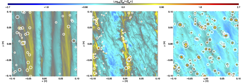
Figure 1: The surface density of solids in the $x$-$y$ (orbital) plane, shown after self-gravity has been turned on and dense clumps have collapsed. From left to right, the panels depict runs with $\tau=0.006$, $\tau=0.3$ and $\tau=2$, at times $105.4\Omega^{-1}$, $7.6\Omega^{-1}$ and $8.8\Omega^{-1}$ after self-gravity has been switched on, respectively. White circles depicts the Hill spheres for a subset of the identified planetesimals. Both the solid surface density structure and the initial positions of planetesimals become more axisymmetric at low values of the stopping time.

Figure 1 shows projections of the surface density of solid material for the three simulation runs in the orbital plane after dense clumps have formed. Visually, they are quite distinct. The prominence of axisymmetric bands in the solid surface density decreases with increasing $\tau$, and notably less material collapses promptly into bound clumps for the $\tau=0.006$ run. In the smaller $\tau$ runs, the planetesimals form primarily in two azimuthally extended bands. In contrast, the planetesimals in the $\tau=2$ run fill the box much more uniformly.

Table 1: Summary of simulation results

$\tau$	$Z$	$p$	$m$
0.006	0.1	1.73 $\pm$ 0.11	1.50 $\pm$ 0.02
0.3	0.02	1.61 $\pm$ 0.08	1.65 $\pm$ 0.10
2.0	0.1	1.54 $\pm$ 0.04	1.62 $\pm$ 0.11

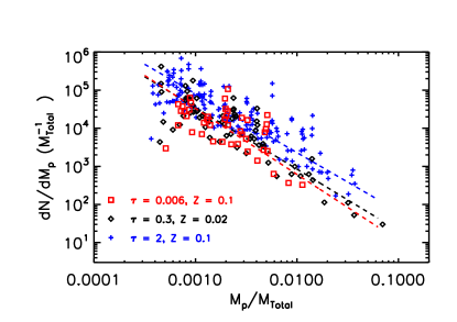
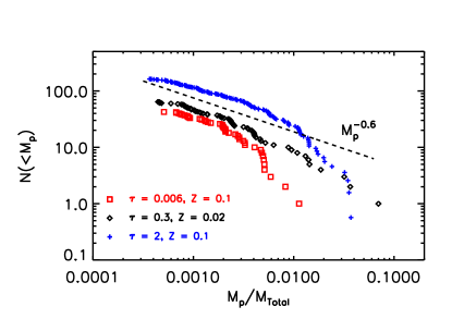
Figure 2: The differential (left) and cumulative (right) initial planetesimal mass function derived from the simulations. In the left plot, the points show unsmoothed “local” estimates of the mass function, and the lines show best-fit solutions derived using a maximum likelihood estimator assuming a power-law form. The simulation with the smallest particles ($\tau=0.006$, red) forms a significantly smaller total mass of planetesimals throughout the duration of the run, but no significant differences in the slope of the derived mass function are observed. The agreement between the points on the low mass end of the cumulative function and the $M_{p}^{-0.6}$ power law (dashed line) demonstrates that at small masses, the mass function is well represented by the single power law fit that we have calculated.

From these snapshots, we use a clump-finding routine to identify and measure the bound masses $M_{{\rm p},i}$ of collapsed objects (we use an identical algorithm to Simon et al., 2016). For visual purposes, we compute an unsmoothed estimate of the differential mass function at masses corresponding to each planetesimal,

$$\left.\frac{{\rm d}N}{{\rm d}M_{\rm p}}\right|_{i}=\frac{2}{M_{{\rm p},i+1}-M_{{\rm p},i-1}},$$ (10)

The resulting mass functions are plotted in the left plot of Figure 2. The shape of the mass functions is generally consistent with a single power-law for all three runs, though, as we discuss in more detail below, there is likely a cut-off at high mass. The single power law fit is clearest in the intermediate and high-$\tau$ runs which form planetesimals with a broader range of masses. Assuming that the data is indeed drawn from a power-law distribution, ${\rm d}N/{\rm d}M_{p}\propto M_{\rm p}^{-p}$, we proceed to estimate the index $p$ and error $\sigma$ using a maximum likelihood estimator (Clauset et al., 2009). Given $n$ planetesimals with masses $M_{{\rm p},i}\geq M_{\rm p,min}$, we have,

$$p = 1+n\left[\sum_{i=1}^{n}\ln\left(\frac{M_{{\rm p},i}}{M_{\rm p,min}}\right)\right]^{-1},$$ (11)

$$\sigma = \frac{p-1}{\sqrt{n}}.$$ (12)

The derived slopes and their associated errors are given in Table 1. Within 1-1.5 $\sigma$ all three runs are consistent with $p=1.6$, as found both in our previous work (Simon et al., 2016) and in Johansen et al. (2015). It is also worth noting that despite the consistent value of $p$, the total fraction of mass converted to planetesimals varies strongly with stopping time; $\sim 10\%$, $40\%$, and $70\%$ of the total mass in solids is converted to planetesimals for the $\tau=0.006,0.3,$ and 2 simulations, respectively. For the smaller mm–cm sized solids present in the inner regions of disks, our results suggest a relatively low planetesimal formation efficiency in these regions.

We also calculate the cumulative mass function, as shown in the right plot of Fig. 2. A power law index of $-0.6$ clearly agrees with the mass function slope for low mass objects. This suggests that the differential mass functions are well fit by a single power law because there is a significantly larger number of planetesimals at small masses, thus weighting the fit towards the small mass end. Therefore, while in reality the mass distribution will have a cut off at some high mass value (which depends on $\tau$), the differential distribution can be well fit by a single power law that is representative of masses away from the cut off.

Finally, we have also examined the evolution of $p$ and the maximum and minimum planetesimal masses (in all the three simulations) for times after which a significant number of planetesimals have formed; the results are shown in Fig. 3. Note that due to limitations with the clump finder algorithm (as described more fully in Simon et al. 2016), we smoothed the curves (with a box car average) to remove noise associated with this algorithm. As the figure shows, $p$ and the minimum planetesimal mass are relatively constant in time , whereas the maximum planetesimal mass grows by a factor of order unity in each simulation, likely due to accretion of smaller particles and/or mergers with smaller planetesimals. Despite this growth the mass function does not evolve appreciably once planetesimals have formed.

Our ability to directly measure any potential dependence of the mass function on particle properties is limited by the relatively small number of collapsed clumps, but across the range of $\tau$ considered, we can bound deviations at the level of $\Delta p\lesssim 0.1-0.2$. We can therefore exclude, with moderately high confidence, the possibility that the streaming instability might result in a steep mass function ($p>2$) with most of the mass in the smallest planetesimals.

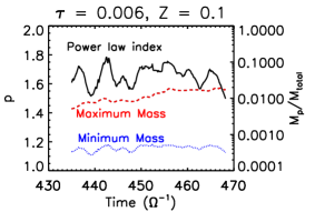
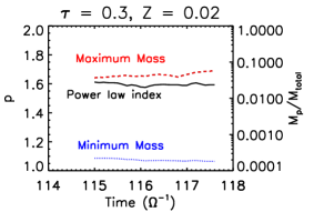
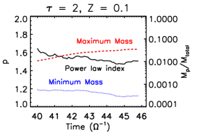
Figure 3: Time evolution of the power law index (solid, black line), maximum planetesimal mass (dashed, red line), and minimum planetesimal mass (dotted, blue line) for the $\tau=0.006$ (left), $\tau=0.3$ (middle), and $\tau=2$ (right) simulations for a period of time after planetesimals have formed. Both the power law index, $p$, and the minimum planetesimal mass are relatively constant in time, whereas the maximum planetesimal mass grows slowly, presumably due to continued accretion of small particles and/or mergers with smaller planetesimals.

4 Particle clustering prior to collapse

The similarity in the mass functions from the different runs is somewhat surprising given the visual differences in the large-scale particle structures that are collapsing (Figure 1). To identify possible differences on smaller spatial scales, we compute the power spectra of the pre-collapse particle density fields. The power spectrum maps uniquely to the mass function in the case where the density is a gaussian random field (Press & Schechter, 1974). In the more complex case relevant here we use the power spectra only to test whether the non-linear structures produced by the streaming instability prior to the onset of self-gravity are indifferent to the particle size.

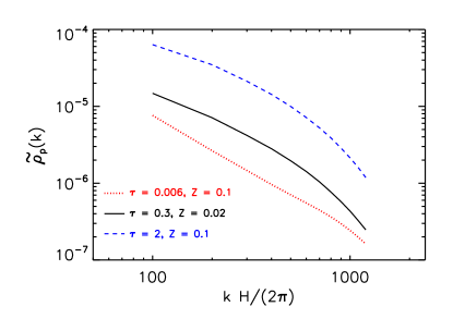
Figure 4: The power spectrum of the particle density field, computed via interpolation on to the hydrodynamic grid in a fixed (across runs) slice centered on the disk mid-plane. The power spectra are computed prior to turning on self-gravity, in the saturated state of the streaming instability. At high $k$ the slopes for the $\tau=0.3$ (black, solid) and $\tau=2$ (blue, dashed) runs are the same, while the run with smaller particles ($\tau=0.006$; red, dotted) is significantly flatter.

Figure 4 shows the three dimensional power spectra $\tilde{\rho}_{p}(k)$ computed from a time slice just before self-gravity is switched on. The thickness of the particle layer at this stage varies substantially with $\tau$ (higher $\tau$ allows for greater settling). To minimize artifacts in the power spectra created by the different thicknesses, we compute $\tilde{\rho}_{p}(k)$ from the interpolated density field $\rho({\bf x})$ in a mid-plane slice whose thickness is chosen to be smaller than the scale height of the thinnest particle layer (for $\tau=2$). The three-dimensional power spectra are then averaged over shells of constant $|{\bf k}|$.

Up to normalization differences the power spectra for all three runs display a high level of similarity. From calculating the largest Hill radius in each run, we expect scales of $kH/2\pi\gtrsim 100$ to seed the collapse.. Fitting a power-law, $\tilde{\rho}_{p}(k)\propto k^{-m}$, to the data at $kH/2\pi>100$, we find that $m\approx 1.5$–$1.7$ with reasonably large errors for the larger two $\tau$ values, with the precise values and their associated errors shown in Table 1. All three runs yield statistically consistent slopes, suggesting that the near-identical mass functions formed from those runs result from commonality in the small-scale particle structures formed in the non-self-gravitating non-linear evolution of the streaming instability. It should be noted, however, that from a visual inspection (Fig. 4) the shape and slope of the power spectrum for $\tau=0.006$ is significantly different (and better fit with a single power law) than for the higher $\tau$ cases, even though their fitted power-law slopes are statistically equal. It is possible that any such differences in the power spectra translate into differences in the mass function at a level that is smaller than our current measurement uncertainties.

5 Discussion

We have presented results from a small number of high resolution simulations of the streaming instability (Youdin & Goodman, 2005) that model the gravitational collapse of over-dense structures toward planetesimals. The simulations were initialized with values of the dimensionless stopping time and local metallicity that promote strong clustering and prompt collapse (Carrera et al., 2015; Yang et al., 2016). For $0.006\leq\tau\leq 2$ we find that the power law part of the resulting mass function (${\rm d}N/{\rm d}M_{p}\propto M_{p}^{-p}$) has an approximately universal slope, $p\simeq 1.6$, consistent with that measured previously for particle sizes in the middle of this range (Johansen et al., 2012; Simon et al., 2016).

The similar planetesimal mass distributions in the different runs is somewhat surprising, given differences in the larger scale geometry of the particle clustering. However, this similarity is consistent with the approximately equal slopes in the power spectra of particle clustering on the smaller scales relevant to collapse. It is possible that the observed differences in the shape of the power spectra would translate into small deviations from universality, but within the uncertainties outlined here, our results strongly support a top-heavy mass function for planetesimals. This finding is consistent with previous streaming instability simulations, but is now shown over a broader range of $\tau$–$Z$ parameter space.

Our ability to directly determine the predicted initial mass function is limited by small number statistics. The statistics could be improved by co-adding samples derived from independent runs, by increasing the spatial resolution, or by increasing the domain size. In Simon et al. (2016), we showed that the planetesimal mass distribution is essentially independent of the time at which self-gravity is turned on in the simulation. However this independence still remains to be tested at higher resolutions and across the broader ranges of parameters considered here.

Where gravitational collapse is encountered in other astrophysical settings, notably in the hydrodynamic formation of stars (Bastian et al., 2010) and in the collision-less collapse of dark matter haloes (Navarro et al., 1997), it is known to exhibit universal features. Planetesimals may in principle form from gravitational collapse via other routes, for example from the direct collapse of dense particle layers (Goldreich & Ward, 1973; Youdin & Shu, 2002; Shi & Chiang, 2013), secular gravitational instability (Youdin, 2011; Takahashi & Inutsuka, 2014) or when vortices accumulate solids (Barge & Sommeria, 1995; Raettig et al., 2015). It is of interest to explore whether these processes lead to similar or identical top-heavy power-law mass functions to those found here, and hence whether constraints on planetesimal formation from the asteroid (Morbidelli et al., 2009) and Kuiper belts (Nesvorný et al., 2010) test specifically the streaming instability or rather a broader class of gravitational collapse scenarios. On the other hand, if the mass function is indeed intimately coupled to the non-linear state of the streaming instability, turbulence driven by other means (e.g., the magnetorotational instability, Balbus & Hawley, 1998) and imposed onto the streaming instability may fundamentally alter the mass function of planetesimals.

References

- Armitage (2015) Armitage, P. J. 2015, ArXiv e-prints (1509.06382)
- Bai & Stone (2010) Bai, X.-N., & Stone, J. M. 2010, ApJ, 722, 1437
- Bai & Stone (2010) Bai, X.-N., & Stone, J. M. 2010, The Astrophysical Journal Letters, 722, L220
- Balbus & Hawley (1998) Balbus, S. A., & Hawley, J. F. 1998, Reviews of Modern Physics, 70, 1
- Barge & Sommeria (1995) Barge, P., & Sommeria, J. 1995, A&A, 295, L1
- Bastian et al. (2010) Bastian, N., Covey, K. R., & Meyer, M. R. 2010, ARA&A, 48, 339
- Birnstiel et al. (2012) Birnstiel, T., Klahr, H., & Ercolano, B. 2012, A&A, 539, A148
- Carrera et al. (2015) Carrera, D., Johansen, A., & Davies, M. B. 2015, A&A, 579, A43
- Clauset et al. (2009) Clauset, A., Shalizi, C. R., & Newman, M. E. J. 2009, SIAM Review, 51, 661
- Flaherty et al. (2015) Flaherty, K. M., Hughes, A. M., Rosenfeld, K. A., et al. 2015, ApJ, 813, 99
- Goldreich & Ward (1973) Goldreich, P., & Ward, W. R. 1973, ApJ, 183, 1051
- Johansen et al. (2014) Johansen, A., Blum, J., Tanaka, H., et al. 2014, Protostars and Planets VI, 547
- Johansen et al. (2015) Johansen, A., Mac Low, M.-M., Lacerda, P., & Bizzarro, M. 2015, Science Advances, 1, 1500109
- Johansen et al. (2007) Johansen, A., Oishi, J. S., Mac Low, M.-M., et al. 2007, Nature, 448, 1022
- Johansen & Youdin (2007) Johansen, A., & Youdin, A. 2007, ApJ, 662, 627
- Johansen et al. (2009) Johansen, A., Youdin, A., & Mac Low, M.-M. 2009, ApJ, 704, L75
- Johansen et al. (2012) Johansen, A., Youdin, A. N., & Lithwick, Y. 2012, A&A, 537, A125
- Koyama & Ostriker (2009) Koyama, H., & Ostriker, E. C. 2009, ApJ, 693, 1316
- Morbidelli et al. (2009) Morbidelli, A., Bottke, W. F., Nesvorný, D., & Levison, H. F. 2009, Icarus, 204, 558
- Navarro et al. (1997) Navarro, J. F., Frenk, C. S., & White, S. D. M. 1997, ApJ, 490, 493
- Nesvorný et al. (2010) Nesvorný, D., Youdin, A. N., & Richardson, D. C. 2010, AJ, 140, 785
- Pinilla et al. (2012) Pinilla, P., Birnstiel, T., Ricci, L., et al. 2012, A&A, 538, A114
- Press & Schechter (1974) Press, W. H., & Schechter, P. 1974, ApJ, 187, 425
- Raettig et al. (2015) Raettig, N., Klahr, H., & Lyra, W. 2015, ApJ, 804, 35
- Schäfer et al. (2017) Schäfer, U., Yang, C.-C., & Johansen, A. 2017, Astronomy and Astrophysics, 597, A69
- Shi & Chiang (2013) Shi, J.-M., & Chiang, E. 2013, ApJ, 764, 20
- Simon et al. (2016) Simon, J. B., Armitage, P. J., Li, R., & Youdin, A. N. 2016, ApJ, 822, 55
- Simon et al. (2015) Simon, J. B., Lesur, G., Kunz, M. W., & Armitage, P. J. 2015, MNRAS, 454, 1117
- Stone & Gardiner (2010) Stone, J. M., & Gardiner, T. A. 2010, ApJS, 189, 142
- Stone et al. (2008) Stone, J. M., Gardiner, T. A., Teuben, P., Hawley, J. F., & Simon, J. B. 2008, ApJS, 178, 137
- Takahashi & Inutsuka (2014) Takahashi, S. Z., & Inutsuka, S.-i. 2014, ApJ, 794, 55
- Weidenschilling (1977) Weidenschilling, S. J. 1977, MNRAS, 180, 57
- Whipple (1972) Whipple, F. L. 1972, in From Plasma to Planet, ed. A. Elvius, 211
- Yang et al. (2016) Yang, C.-C., Johansen, A., & Carrera, D. 2016, ArXiv e-prints
- Youdin & Johansen (2007) Youdin, A., & Johansen, A. 2007, The Astrophysical Journal, 662, 613
- Youdin (2011) Youdin, A. N. 2011, ApJ, 731, 99
- Youdin & Chiang (2004) Youdin, A. N., & Chiang, E. I. 2004, ApJ, 601, 1109
- Youdin & Goodman (2005) Youdin, A. N., & Goodman, J. 2005, ApJ, 620, 459
- Youdin & Shu (2002) Youdin, A. N., & Shu, F. H. 2002, ApJ, 580, 494