What is the right theory for Anderson localization of light?

Abstract

Anderson localization of light is traditionally described in analogy to electrons in a random potential. Within this description the disorder strength – and hence the localization characteristics – depends strongly on the wavelength of the incident light. In an alternative description in analogy to sound waves in a material with spatially fluctuating elastic moduli this is not the case. Here, we report on an experimentum crucis in order to investigate the validity of the two conflicting theories using transverse-localized optical devices. We do not find any dependence of the observed localization radii on the light wavelength. We conclude that the modulus-type description is the correct one and not the potential-type one. We corroborate this by showing that in the derivation of the traditional, potential-type theory a term in the wave equation has been tacititly neglected. In our new modulus-type theory the wave equation is exact. We check the consistency of the new theory with our data using a field-theoretical approach (nonlinear sigma model).

Anderson localization, i.e. the possibility of an arrest of the motion of an electronic wave packet in a disordered environment, has fascinated researchers since the appearance of Anderson’s 1958 article ¹. In 1979 it became clear ² that this phenomenon is due to destructive interference of recurrent scattering paths and led - via the one-parameter scaling hypothesis - to the conclusion that in disordered one- and two-dimensional systems the waves are always localized. This scaling theory was put on solid theoretical grounds by relating the Anderson scenario to the nonlinear sigma model of planar magnetism ^{3; 4; 5} and by the self-consistent diagrammatical localization theory ^{6; 7; 8}. It became clear that this transition should exist in any physical system governed by a wave equation with disorder ⁹.

Anderson localization has gained much attention recently in wave optics¹⁰ due to a large number of possible applications reaching from solar cells to endoscopic fibres^{11; 12; 13}.

In the description of possible localization of light by means of the nonlinear-sigma-model theory John ^{14; 15; 16} adopted the same structure of a classical wave equation with disorder as in his sound-wave theory ^{17; 18}, namely a fluctuating coefficient of the double time derivative. In the time-Fourier-transformed version of the wave equation this version had the attractive feature that a one-to-one mapping to the Schrödinger equation of an electron in a random potential could be established. So most of the results of the theory for the electronic Anderson localization could be taken over ^{14; 15; 16; 19; 20; 8}. We call this approach the “potential-type” description (PT).

On the other hand, in an alternative formulation, used successfully for the vibrational anomalies in glasses ^{21; 22; 23} the disorder enters the coefficient of the spatial derivatives, which in the case of sound waves is the elastic modulus, in the case of electromagnetic waves the the dielectric modulus $1/\epsilon({\bf r})$. We call this the “modulus-type” description (MT).

While the existence of Anderson localization of light in 3-dimensional optical materials is still under debate ^{24; 25}, in optical systems with restricted dimensionality one has nowadays evidence for Anderson localization, in particular in optical fibers with transverse disorder ^{26; 27; 13}. The possibility of observing transverse localization of light in optical fibers, which are translation invariant along the fiber axis but exhibit disorder in one or two of the transverse directions, was already predicted some time ago ^{28; 29}.

In fibers composed of microfibers with different dielectric constants the presence of transverse localization leads to the existence of channels with the diameter of the transverse localization length, which transmit light like in a micro-waveguide. As the localized modes have been proven to be of single-mode character ³⁰, such fibers are extremely useful for transfer of multiple information, e.g for endoscopy.

The theoretical description of transverse Anderson localization in fibers with transverse disorder ^{29; 27; 31} followed the potential-type approach. This description results in a rather strong dependence of the localization lengths on the wavelength of the applied light ³¹.

In the present contribution we show that this description is not consistent with our experimental observation. We have measured the localization lengths of fibers with transverse disorder as a function of the light wavelength and do not find any change with wavelength. Motivated by this observation, we adopted the modulus-type approach do disorder and found perfect consistency with the experiments. We conclude that the modulus-type description is the correct theory for Anderson localization of light. A further argument against the potential-type approach is that within this model the fibers are opaque in the longitudinal ($z$) direction. Due to the Rayleigh-scattering mechanism this is not the case in the modulus-type theory, in which the samples are transparent in the $z$ direction.

In the frequency regime (with frequency variable $\omega=2\pi c_{0}/\lambda\sqrt{\langle\epsilon\rangle}=c_{0}k_{0}/\sqrt{\langle\epsilon\rangle}$, where $c_{0}$ is the vaccum light speed, $\lambda$ is the wavelength $k_{0}=2\pi/\lambda$ is the wavenumber and $\langle\epsilon\rangle$ the average permittivity) the two conflicting stochastic wave equations, which are both considered to be derived from Maxwell’s equations with inhomogeneous permittivity, take the form

$$\big{[}\tilde{\epsilon}({\bf r})k_{0}^{2}+\nabla^{2}\big{]}E_{\alpha}({\bf r},\omega) = 0\qquad\qquad\mbox{PT}$$

$$\big{[}k_{0}^{2}+\nabla\frac{1}{\tilde{\epsilon}({\bf r})}\nabla\big{]}B_{\alpha}({\bf r},\omega) = 0\qquad\qquad\mbox{MT}$$ (1)

$E_{\alpha},B_{\alpha}$ are components of the electric, magnetic field, resp. and $\tilde{\epsilon}({\bf r})=\epsilon({\bf r})/\langle\epsilon\rangle$ denotes the relative fluctuations of the dielecric constant. In what follows we disregard the vector character of the electromagnetic fields.

In the case of transverse disorder $\epsilon$ fluctuates only in the $x,y$ direction, so one can perform a Fourier transform with respect to the $z$ direction ($\partial/\partial z\rightarrow ik_{z}$) to obtain

$$\big{[}{\cal E}+k_{0}^{2}\Delta\tilde{\epsilon}({\bm{\rho}})+\nabla_{\bm{\rho}}^{2}\big{]}E_{\alpha}(k_{z},{\bm{\rho}},\omega) = 0\qquad\mbox{PT}$$

$$\big{[}{\cal E}+\nabla_{\bm{\rho}}\frac{1}{\tilde{\epsilon}({\bf r})}\nabla_{\bm{\rho}}\big{]}B_{\alpha}(k_{z},{\bm{\rho}},\omega) = 0\qquad\mbox{MT}$$ (2)

with ${\bm{\rho}}=x{\bf e}_{x}+y{\bf e}_{y}$ and $\Delta\tilde{\epsilon}({\bm{\rho}})=\tilde{\epsilon}({\bm{\rho}})-1$. Here we have introduced the spectral parameter (eigenvalue) ${\cal E}=k_{\perp}^{2}=k_{0}^{2}-k_{z}^{2}=k_{0}^{2}\sin(\theta)^{2}$, where $\theta$ is the azimuthal angle.

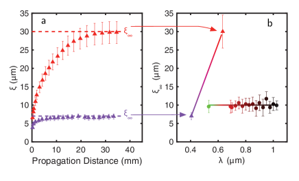
Figure 1: a: Localisation radius $\xi(z)$ as a function of the distance $z$ along the fibre for the two light wavelengths $\lambda=0.4\,\mu$m and $\lambda=0.63\,\mu$m from the simulation of Karbasi³¹ based on the potential-type version of Eqs. (What is the right theory for Anderson localization of light?).
b: Measured averaged localization length of fibres with transverse disorder as a function of the incident-laser wavelength (full circles), compared with the two values $\xi_{\infty}\equiv\xi(z=\infty)$ of panel a (full triangles).

We note that in the PT equation the wavenumber $k_{0}=2\pi/\lambda$ appears as an external parameter in front of the fluctuating permittivity, whereas in the MT version $k_{0}$ enters only via the spectral parameter ${\cal E}$.

In the paraxial limit $\theta\rightarrow 0$ ${\cal E}$ can approximated by $-2k_{0}\Delta k_{z}$, where $\Delta k_{z}=k_{z}-k_{0}$ is the Fourier wavenumber corresponding to the $z$ dependence of the envelopes $E_{\alpha}^{(0)},B_{\alpha}^{(0)}$ of the electromagnetic fields. Transformed back to the $z$ dependence of the envelope one obtains

$$\big{[}2ik_{0}\frac{\partial}{\partial z}+k_{0}^{2}\Delta\tilde{\epsilon}({\bm{\rho}})+\nabla_{\bm{\rho}}^{2}\big{]}E_{\alpha}^{(0)}(z,{\bm{\rho}},\omega) = 0\quad\mbox{PT}$$

$$\big{[}2ik_{0}\frac{\partial}{\partial z}+\nabla_{\bm{\rho}}\frac{1}{\tilde{\epsilon}({\bf r})}\nabla_{\bm{\rho}}\big{]}B^{(0)}_{\alpha}(z,{\bm{\rho}},\omega) = 0\quad\mbox{MT}$$ (3)

Eqs. (What is the right theory for Anderson localization of light?) are mathematically equivalent to a time-dependent Schrödinger equation (with “time” $z/2k_{0}$).

The PT version of Eqs. (What is the right theory for Anderson localization of light?) has been used in Refs. ^{29; 26; 27; 31} for a numerical calculation of the localization properties of transverse-disordered optical fibres. In the panel a of Fig. 1 we have reproduced the $z$ dependence of the radius of the localization lengths $\xi(z)$, obtained by such a simulation³¹ for two different light wavelengths $\lambda$, wich saturate for large $z$ at the localization length $\xi(z\!=\!\infty)\equiv\xi_{\infty}$. The strong dependence on the wavelength is striking.

In order to check, whether this behaviour predicted by the PT theory is realistic, we have taken samples composed of microfibres with different permittivity (polystyrene, PS $\epsilon_{\rm PS}/\epsilon_{0}=1.59$, polymethylmethacrylate, PMMA, $\epsilon_{\rm PMMA}/\epsilon_{0}=1.49$), fabricated as described in ²⁷ in which transverse localization is observed^{27; 31; 32; 33}. We measured the localization length in such devices by injecting a focused (order of a micrometer) monocromatic light at the fibre input tip while monitoring the total fibre output. The average extent of the output intensity pattern is determined by the localization length in the fibre. Thus we estimated it by determining the first spatial moment of the intensity distribution. Averaging is performed by scanning the input facet with a 3-axis piezo motor sustaining the fibre. The experimental setup together with a sketch of the fibre geomety is shown in Fig. 2. A more detailed description of our experiment can be found in the supplemental material.

In panel b of Fig. 1 we show our data for the localization length $\xi_{\infty}$ (full circles), averaged over all modes and three samples as a function of the incident laser wavelength. It can be seen that there is no change with the wavelength.

Our interpretation is that this discrepancy is due to the inadequateness of the potential-type stochastic wave equation.

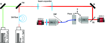
Figure 2: Sketch of the experimental setup: The light from a ND:YAG or a Ti:Sapphire laser is coupled to the fibre by using objective OBJ 1. The back-reflected light is then visualized by the camera CCD1 through the beamsplitter BS in order to perform the fine tuning of the alignment. The piezo devices control the laser injection location. The transmitted light is collected by the objective OBJ2 ad imaged on camera CCD2 with a magnification of 50.
In (a) a sketch of the fibre is reported, while in (b) a magnified image of the fibre tip surface is shown, where polymethylmethacrylate appears dark and polystyrene white.

But how come that the results of the two descriptions, which are both supposed to arise from Maxwell’s equation with spatially varying permittivity, differ from each other? For deriving the wave equations in the presence of an inhomogeneous permittivity $\epsilon({\bf r})$ one can either solve for the electrical field ${\bf E}({\bf r},t)$ (PT) or divide through $\epsilon({\bf r})$ and then solve for the magnetic field ${\bf B}({\bf r},t)$ (MT). In the first case one has to decompose the double curl of ${\bf E}$, whereas in the second case the double curl of ${\bf B}$:

$$\frac{\epsilon({\bf r})}{c_{0}^{2}}\frac{\partial^{2}}{\partial t^{2}}{\bf E}({\bf r},t) = -\nabla\times\nabla\times{\bf E}({\bf r},t)\qquad\mbox{PT}$$

$$= \nabla^{2}{\bf E}-\nabla\big{(}\nabla\cdot{\bf E}({\bf r},t)\big{)}$$

$$\frac{\partial^{2}}{\partial t^{2}}{\bf B}({\bf r},t) = -\nabla\times\frac{c_{0}^{2}}{\epsilon({\bf r})}\nabla\times{\bf B}({\bf r},t)\qquad\mbox{MT}$$ (4)

$$= \nabla\cdot\frac{c_{0}^{2}}{\epsilon({\bf r})}\cdot\nabla{\bf B}({\bf r},t)$$

In the absence of free charges but in the presence of a spatially fluctuating dielectric constant we get for the divergence of the electic field

$$\nabla\cdot{\bf E}=-\frac{1}{\epsilon_{0}}\nabla\cdot{\bf P}=-\frac{1}{\epsilon_{0}}\nabla\cdot[\epsilon({\bf r})-\epsilon_{0}]{\bf E}$$ (5)

from which follows³⁴

$$\nabla\cdot{\bf E}=-\frac{1}{\epsilon({\bf r})}{\bf E}\cdot\nabla\epsilon({\bf r})\neq 0$$ (6)

The divergence of ${\bf B}$, on the other hand, is zero.

Obviously, in the first paper using the PT approach¹⁴ and the whole following literature^{15; 16; 20; 29; 26; 27; 31; 35} the divergence of ${\bf P}$ (which describes the frozen-in displacement charges) had been tacitly assumed to be zero. We believe that this is the origin of the discrepancy of the two theories.

We further check the consistency or otherwise of the two approaches by applying the theory of the nonlinear sigma model of localization to the stochastic Helmholtz equations (What is the right theory for Anderson localization of light?). Wegner³ realized that the nonlinear sigma model of planar ferromagnetism obeys the same scaling of the coupling constant with the length scale $L$ as the conductance $g$ of electrons in the scaling theory of localization², namely

$$\frac{dg}{d\ln L}=g\beta(g)=(d-2)g-c$$ (7)

where $d$ is the dimensionality and $c$ is a constant of order unity. Later a rigorous mapping of the field-theoretical representation of the configurationally averaged Green’s functions to a generalized nonlinear sigma model was established^{4; 37; 5}. This was then adapted to classical sound waves^{17; 22}, and – using the PT approach – to electromagnetic waves^{14; 15; 16}. For $d=2$ the solution of Eq. (7) is

$$g(L)=g(L_{0})-c\ln(L/L_{0})$$ (8)

where $L_{0}$ is the reference length scale, i.e. $g$ scales always towards zero. The localization length $L\equiv\xi_{\infty}$ is the length at which $g=1$^{5; 17}, and $g(L_{0})=g_{0}$ is the reference conductance.

The nonlinear-sigma-model theory provides us via a saddle-point approximation with a nonperturbative way to calculate the reference conductance, which is related to the scattering mean-free path $\ell_{0}({\cal E})$. Within this saddle-point approximation (self-consistent Born approximation, SCBA^{17; 22}) $g_{0}({\cal E})$ and $\ell_{0}({\cal E})$ are given in terms of a complex self-energy function $\Sigma(s)=\Sigma^{\prime}({\cal E})+i\Sigma^{\prime\prime}({\cal E})$ with complex spectral parameter $s={\cal E}+i\eta,\eta\rightarrow 0$

$$\ln\xi_{\infty}({\cal E})\propto g_{0}({\cal E}) = \frac{{\cal E}+k_{0}^{2}\Sigma^{\prime}({\cal E})}{k_{0}^{2}\Sigma^{\prime\prime}({\cal E})}\qquad\quad\,\,\,\mbox{PT}$$

$$\ln\xi_{\infty}({\cal E})\propto g_{0}({\cal E}) = \frac{1-\Sigma^{\prime}({\cal E})}{\Sigma^{\prime\prime}({\cal E})}\qquad\quad\mbox{MT}$$ (9)

The function $\Sigma(s)$ obeys the self-consistent equation

$$\Sigma(s) = \gamma\frac{k_{0}^{2}}{q_{c}^{2}}\int_{0}^{q_{c}}\!\!q\,dq\,{\sf G}(q,s)\qquad\qquad\mbox{PT}$$

$$\Sigma(s) = \gamma\frac{1}{q_{c}^{2}}\int_{0}^{q_{c}}\!\!q\,dq\,q^{2}{\sf G}(q,s)\qquad\qquad\mbox{MT}$$ (10)

with the disorder parameter $\gamma=\langle(\Delta\tilde{\epsilon})^{2}\rangle$ and the averaged one-particle Green’s functions

$${\sf G}(q,s) = \frac{1}{-s-k_{0}^{2}\Sigma(s)+q^{2}}\equiv\frac{1}{-k_{\Sigma}(s)^{2}-q^{2}}\,\,\mbox{PT~{}~{}~{}}$$

$${\sf G}(q,s) = \frac{1}{-s+q^{2}[1-\Sigma(s)]}\equiv\frac{[1-\Sigma(s)]^{-1}}{-k_{\Sigma}(s)^{2}-q^{2}}\,\,\mbox{MT~{}~{}~{}}$$ (11)

where we have introduced a complex wavenumber $k_{\Sigma}(s)=k_{\Sigma}^{\prime}({\cal E})+ik_{\Sigma}^{\prime\prime}({\cal E})$ in an obvious way. The imaginary part of this quantity is related to the scattering mean-free path by $\ell_{0}({\cal E})=1/2k_{\Sigma}({\cal E})^{\prime\prime}$ and we obtain for both descriptions (see ^{17; 22} and the supplementary material)

$$g_{0}({\cal E})=k^{\prime}_{\Sigma}({\cal E})\ell_{0}({\cal E})$$ (12)

The upper $q$ integration limit is given by the correlation parameter $q_{c}=2\pi/L_{c}$^{18; 38}, where $L_{c}$ is the disorder correlation length ($\sim$ diameter of the grains with different permittivities).

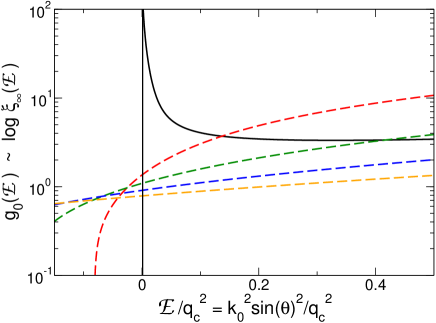
Figure 3: “Conductance” $g_{0}({\cal E})\propto\ln{\xi_{\infty}({\cal E})}$, where $\xi_{\infty}({\cal E})$ is the localization lenght, for the modulus-type description (continuous line) and for the potential-type description (dashed lines) with four different wavelengths $\lambda=1\mu{\rm m},\lambda=0.75\mu{\rm m},\lambda=0.6\mu{\rm m},\lambda=0.5\mu{\rm m}$. For both calculations we used the disorder parameter $\gamma$ = 0.2. The correlation parameter $k_{c}$ has been determined from the spatial distribution of the dielectric constants, see Fig. 2, by an image-processing correlation analysis to be $k_{c}=8\,[\mu{\rm m}]^{-1}$.

In Fig. 3 we show the reference conductance $g_{0}({\cal E})$, which is proportional to the logarithm of the localization length $\xi_{\infty}({\cal E})$, for the two alternative theories against the spectral parameter ${\cal E}$. As to be expected, the $g({\cal E})$ curves depend strongly on $k_{0}$ for the PT model, in contrast to the MT case, in which the $g({\cal E})$ curves do not depend on the wavelength. In this case the only dependence on $k_{0}$ is via the spectral parameter ${\cal E}$. From this it follows that in the MT case the distribution of localization lengths (and hence their average) do not depend on the wavelength, in agreement with our data displayed in Fig. 1b and in disagreement with the numerical (Fig. 1a) and field-theoretical (Fig. 3) predictions of the PT theory.

As reference length scale $L_{0}$ we use the disorder correlation length $L_{c}$ and not the scattering mean-free path^{39; 6}. With $L_{c}\approx$ 1$\mu$m this is consistent with our measured values of $\xi_{\infty}\approx$ 10 $\mu$ corresponding to $g_{0}\approx 5$, which is obtained near ${\cal E}/q_{c}^{2}\approx 0.07$. This value of ${\cal E}$ is well inside the maximum value of $[{\cal E}/q_{c}^{2}]_{\rm max}=0.5L_{c}^{2}/\lambda^{2}$ of our device, determined by $\theta_{\rm max}=50^{\circ}$.

Within the modulus-type description the reference conductance diverges as ${\cal E}^{-1}$ for ${\cal E}\rightarrow 0$. For the mean-free path one obtains $\ell_{0}({\cal E})\propto{\cal E}^{-3/2}$, which is equivalent to a two-dimensional Rayleigh law. This absence of scattering for rays entering the sample exactly in the $z$ direction indicates that the sample is lengthwise transparent, as it should. The Rayleigh law can also be written as $\ell_{0}\propto(\lambda_{\perp}/L_{c})^{3}$, where $\lambda_{\perp}=\lambda/\sin\theta$ is the transverse wavelength. So if $\lambda_{\perp}$ becomes much larger than the grain size $L_{c}$, there is no scattering and hence no localization.

On the contrary, within the potential-type description the sample is predicted to be opaque in the $z$ direction, and the Rayleigh law is absent. It is even seen from Fig. 3, that the spectral scattering intensity of the potential-type model extends into the negative ${\cal E}$ range, rendering the spectrum unstable. Stability, i.e. the restriction of the spectrum to positive values, is however required for disordered bosonic systems⁴⁰.

We see that the previous theoretical approach, the potential-type one, leads to general inconsistencies and, in particular, to an inconsistency with our measured localization data. This is not the case with the modulus-type description, which leads to a positive spectrum, predicts transparency in the $z$ direction and is consistent with our mesured data on transversely localized optical devices. Thus we are convinced that we have now established a sound theoretical fundament for further work on Anderson localization of light.

References

- Anderson (1958) P. W. Anderson, Phys. Rev. 109, 1492 (1958).
- Abrahams et al. (1979) E. Abrahams, P. W. Anderson, D. C. Licciardello, and T. V. Ramakrishnan, Phys. Rev. Lett. 42, 673 (1979).
- Wegner (1979) F. Wegner, Z. Phys. B 35, 207 (1979).
- Schäfer and Wegner (1980) L. Schäfer and F. Wegner, Zeitschrift für Physik B Condensed Matter 38, 113 (1980).
- McKane and Stone (1981) A. J. McKane and M. Stone, Ann. Phys. (N. Y.) 131, 36 (1981).
- Vollhardt and Wölfle (1980) D. Vollhardt and P. Wölfle, Physical Review Letters 45, 842 (1980).
- Vollhardt and Wölfle (1982) D. Vollhardt and P. Wölfle, Phys. Rev. Lett. 48, 699 (1982).
- Wölfle and Vollhardt (2010) P. Wölfle and D. Vollhardt, International Journal of Modern Physics B 24, 1526 (2010).
- Evers and Mirlin (2008) F. Evers and A. D. Mirlin, Rev. Mod. Phys. 80, 1355 (2008).
- John (1991) S. John, Physics Today 44, 32 (1991).
- C. M. Soukoulis, ed. (2001) C. M. Soukoulis, ed., Photonic crystals and light localization in the 21th century (Springer-Science + Business Media, Dordrecht, 2001).
- Wiersma (2013) D. S. Wiersma, Nature Photonics 7, 188 (2013).
- Segev et al. (2013) M. Segev, Y. Silverberg, and D. N. Christodoulides, Nature Photonics 7, 197 (2013).
- John (1984) S. John, Phys. Rev. Lett. 53, 2169 (1984).
- John (1985) S. John, Phys. Rev. B 31, 304 (1985).
- John (1987) S. John, Phys. Rev. Lett. 58, 2486 (1987).
- John et al. (1983) S. John, H. Sompolinsky, and M. J. Stephen, Phys. Rev. B 27, 5592 (1983).
- John and Stephen (1983) S. John and M. J. Stephen, Phys. Rev. B 28, 6358 (1983).
- Kroha et al. (1993) J. Kroha, C. M. Soukoulis, and P. Wölfle, Phys. Rev. B 47, 11093 (1993).
- Sheng (2006) P. Sheng, Introduction to Wave Scattering, Localization and Mesoscopic Phenomena (Springer, Heidelberg, 2006).
- Schirmacher et al. (2004) W. Schirmacher, E. Maurer, and M. Pöhlmann, Phys. Stat. Sol. (c) 1, 92 (2004).
- Schirmacher (2006) W. Schirmacher, Europhys. Letters 73, 892 (2006).
- Schirmacher et al. (2007) W. Schirmacher, G. Ruocco, and T. Scopigno, Phys. Rev. Lett. 98, 025501 (2007).
- Skipetrov and Page (2016) S. E. Skipetrov and J. H. Page, New J. Physics 18, 021001 (2016).
- Sperling et al. (2016) T. Sperling, L. Schertel, M. Ackermann, G. J. Aubry, C. M. Aegerter, and G. Maret, New J. Physics 18, 013039 (2016).
- Schwartz et al. (2007) T. Schwartz, G. Bartal, S. Fishman, and M. Segev, Nature 446, 52 (2007).
- Karbasi et al. (2012a) S. Karbasi, C. R. Mirr, P. G. Yarandi, R. J. Frazier, K. W. Koch, and A. Mafi, Opt. Lett. 37, 2304 (2012a).
- Abdullaev and Abdullaev (1980) S. S. Abdullaev and F. K. Abdullaev, Izv. Vuz. Radiofiz. 23, 766 (1980).
- De Raedt et al. (1989) H. De Raedt, A. Lagendijk, and P. de Vries, Phys. Rev. Lett. 62, 47 (1989).
- Ruocco et al. (2016) G. Ruocco, B. Abaie, A. Mafi, W. Schirmacher, and M. Leonetti, Nature communications (2016), in print.
- Karbasi et al. (2012b) S. Karbasi, C. R. Mirr, R. J. Frazier, P. G. Yarandi, K. W. Koch, and A. Mafi, Opt. Express 20, 18692 (2012b).
- Leonetti et al. (2014) M. Leonetti, S. Karbasi, A. Mafi, and C. Conti, Phys. Rev. Lett. 112, 193902 (2014).
- Karbasi et al. (2013a) S. Karbasi, K. W. Koch, and A. Mafi, Opt. Express 21, 305 (2013a).
- Saleh and Teich (1991) B. E. A. Saleh and M. C. Teich, Fundamentals of photonics (Wiley, New York, 1991), see Chapter 5, Equation (5.2-14).
- Abaie and Mafi (2016) B. Abaie and A. Mafi, Phys. Rev. B 94, 064201 (2016).
- Karbasi et al. (2013b) S. Karbasi, K. W. Koch, and A. Mafi, J. Opt. Soc. Am. B 30, 1452 (2013b).
- Houghton et al. (1980) A. Houghton, A.Jevicki, R. Kenway, and A. M. M. Pruisken, Phys. Rev. Lett 45, 349 (1980).
- Schirmacher et al. (2008) W. Schirmacher, B. Schmid, C. Tomaras, G. Viliani, G. Baldi, G. Ruocco, and T. Scopigno, physica status solidi (c) 5, 862 (2008).
- Lee and Ramakrishnan (1985) P. A. Lee and T. V. Ramakrishnan, Rev. Mod. Phys. 57, 287 (1985).
- Lück et al. (2006) T. Lück, H.-J. Sommer, and M. R. Zirnbauer, J. Math. Phys. 47, 103304 (2006).