Exponential Families for Bayesian Quantum Process Tomography

Abstract

A Bayesian approach to quantum process tomography has yet to be fully developed due to the lack of appropriate probability distributions on the space of quantum channels. Here, by associating the Choi matrix form of a completely positive, trace preserving (CPTP) map with a particular space of matrices with orthonormal columns, called a Stiefel manifold, we present two parametric probability distributions on the space of CPTP maps that enable Bayesian analysis of process tomography. The first is a probability distribution that has an average Choi matrix as a sufficient statistic. The second is a distribution resulting from binomial likelihood data that enables a simple connection to data gathered through process tomography experiments. To our knowledge these are the first examples of continuous, non-unitary random CPTP maps, that capture meaningful prior information for use in Bayesian estimation. We show how these distributions can be used for point estimation using either maximum a posteriori estimates or expected a posteriori estimates, as well as full Bayesian tomography resulting in posterior credibility intervals. This approach will enable the full power of Bayesian analysis in all forms of quantum characterization, verification, and validation.

I Introduction

In the quest to develop quantum technologies, precise characterization of quantum systems is critical to understanding and mitigating noise and imperfections. To date, nearly all quantum characterization techniques such as randomized benchmarking (RB) Knill et al. (2008), quantum state and process tomography (see e.g. Refs. Jones (1994); Chuang and Nielsen (1997); Poyatos et al. (1997); Merkel et al. (2013); Blume-Kohout et al. (2016)), gate-set tomography (GST) Merkel et al. (2013); Blume-Kohout et al. (2016), or even more advanced techniques such as quantum noise spectroscopy Yuge et al. (2011); Álvarez and Suter (2011) tend to primarily rely on a frequentist approach where a large number of experimental data-points are taken in order to estimate the average of some parameter or parameters of interest. As error-rates continue to march lower, having precise knowledge of uncertainties in the estimated parameters is key to improving devices below the fault-tolerant threshold needed for large-scale quantum computing.

To get a sense of the estimation accuracy and to reduce experimental costs, Bayesian-based approaches for RB Granade et al. (2015); Hincks et al. (2018) process tomography Granade et al. (2016); Teo et al. (2018), and noise spectroscopy Ferrie et al. (2018) have been proposed. Despite this intense interest, a fully Bayesian approach to quantum process tomography with analytic prior and posterior distributions has yet to be developed, with the current approaches relying on importance sampling and simple proposal distributions Granade et al. (2016).

A key requirement for Bayesian estimation is having a probability distribution or distributions defined on the relevant space of interest. Furthermore it is generally desired that these distributions can be parameterized in some manner that allows for the capture of meaningful prior information. Typically, this amounts to some form of location and scale parameters. As an example the normal distribution is defined on the space of real numbers and is fully parameterized by a mean and variance. In the context of quantum process tomography, one particular sample space of interest is the space of completely positive and trace preserving (CPTP) maps (see e.g. Nielsen and Chuang (2010)). Therefore, a probability distribution on the space of CPTP maps, preferably with a simple parameterization, could enable fully Bayesian quantum process tomography.

Perhaps the simplest and most familiar example of a random quantum operation are Pauli error channels, commonly used in quantum error correction simulations (see e.g. Aaronson and Gottesman (2004); Knill (2005); Gutiérrez et al. (2013)). On one hand, the average of these distributions is well defined and simple to calculate, allowing them to be used in the analysis of noisy quantum circuits. Their application in Bayesian setting is limited, however. These distributions are fundamentally discrete, and thus are not absolutely continuous with respect to the entire space of CPTP maps and as such will necessarily produce estimates that are Pauli channels and cannot capture error effects such as coherent rotations and non-unital errors that will show up in any non-idealized tomographic procedure. A slight generalization of this concept is discrete mixtures over a finite set of CPTP maps Audenaert and Scheel (2008), which has the same issues as Pauli error channels in the Bayesian context.

More exotic examples of probability distributions on the space of CPTP maps come from the field of random matrix theory. Projections of Haar-random unitaries from a unitary group of higher dimension has been used to define a distribution on the space of CPTP maps that is absolutely continuous on the space of CPTP maps Bruzda et al. (2009). This essentially provides a uniform distribution of CPTP maps with a given Kraus rank. Ref. Collins and Nechita (2016) further provides a useful review on a number of results on random CPTP maps derived from random unitary operations, along with a number of theoretical results on their composition and effect on quantum states. The downside to these approaches is that there is no particularly useful parameterization in terms of a location and scale parameter. In fact the average of these distributions is the maximally mixed channel. This is not particularly useful as a prior for a high-fidelity quantum channel, which is what one requires when characterization quantum devices. That said, the distribution of Bruzda et al. (2009) has been used as a proposal distribution for process tomography in Pogorelov et al. (2017) using similar importance sampling techniques as in Granade et al. (2016). The efficiency of this approach would be greatly enhanced by a proposal distribution that can capture meaningful prior information, such as the distributions introduced below.

In contrast to the above approaches, here we demonstrate two approaches to generating probability distributions relevant to quantum process tomography. The first is a family of probability distributions of random CPTP maps that are absolutely continuous and completely characterized by their first moment, in this case, an average Choi matrix. The second is an alternative formulation where these distributions can be characterized as maximum entropy distributions with a given average value. Our approach makes use of the theory of exponential families on the manifold of matrices with orthonormal columns, known as Stiefel manifolds James (1976).

Our first approach is natural to consider in the context of noisy quantum systems. On one hand, the evolution of an open quantum system can often be treated as a noisy evolution, through the stochastic Liouville equation Kubo (1963). This type of description applies to some of the most common types of qubits and their predominant decoherence mechanisms (see e.g. Refs. Kubo (1957); Schulten and Wolynes (1978); Ernst et al. (1987); Schneider and Milburn (1998); Grigorescu (1998); Abergel and Palmer (2003); Cheng and Silbey (2004); Wilhelm et al. (2007)). On the other hand, especially in the context of quantum gates or circuits, we often speak of just an average error channel (or simply “the” error channel) for a given quantum operation, and do not consider it as either a random variable or stochastic process. In this context, quantum process tomography is essentially computing estimates of the average quantum channel. This motivates the desire for a parametric probability distribution for which the average map, as estimated from tomography or simulation, is a sufficient statistic. This approach provides such a parameterization.

The second approach is derived from the likelihood of a process tomographic experiment using the same manifold of matrices with orthonormal columns. This in turn allows for construction of a second class of prior based on the conjugate prior for binomial data. In effect, this prior uses synthetic “pseudo-experiments” to capture prior information about the distribution of CPTP maps. Since this distribution is derived from the likelihood of binomial data, it is also the posterior distribution for binomial process tomographic data. Using a sampling scheme adapted from Hoff (2009), we show how these two priors can be combined to perform Bayesian process tomography for both point estimation and for generating full posterior distributions. This allows one to efficiently include prior information from techniques such as RB into process tomography experiments.

In the following sections, we relate known properties of CPTP maps to Stiefel manifolds and show how this representation is compatible with process tomography. Next we review definitions from classical statistics and introduce the concept of an exponential family of probability distributions, and derive two families on the Stiefel manifold for the purposes of Bayesian process tomography. Following this, we show how these distributions can be used to generate Bayesian estimates for process tomography, and compare the results to traditional maximum likelihood methods.

II CPTP Maps and Stiefel Manifolds

In quantum information, a quantum state can be represented by a density operator $\rho$, where $\rho\in\mathbb{C}^{N\times N}$ is a positive semi-definite, Hermitian matrix with $\operatorname{Tr}(\rho)=1$. Quantum operations are then completely positive, trace-preserving (CPTP) maps Nielsen and Chuang (2010). In this work, we will make the additional assumption that the quantum maps of interest map to density operators of the same dimension as the input dimension, but this can be generalized. CPTP maps can be represented by the Choi matrix form $\Lambda$, which can be derived from a Liouvillian superoperator $\mathcal{L}$ via a coordinate shuffling involution operation Bruzda et al. (2009); Wood et al. (2015). The relevant properties of $\Lambda$ that we will consider here are 1) the CP property implies $\Lambda$ is Hermitian and postive-semidefinite, and 2) the TP property implies that $\operatorname{Tr}_{B}\Lambda=I_{N}$, where $\operatorname{Tr}_{B}$ denotes the partial trace over the second subsystem when $\Lambda$ is viewed as an operator in the tensor product space of two $N\times N$ spaces. Since $\Lambda$ is Hermitian and positive semidefinite, there exists a matrix $S$ such that $\Lambda=S^{\dagger}S$, i.e., a square root factorization. Note that this factorization is not unique, indeed $US$ for any unitary $U$ of appropriate dimension will result in an identical Choi matrix as $S$. Furthermore, even the dimension of $S$ is not unique as the rank $K$ of $\Lambda$ (i.e., the Kraus rank) implies that $S$ can be expressed as a $K\times N^{2}$ complex matrix, but there exist $M\times N^{2}$-dimensional matrix factorizations for all $M\geq K$. Regardless of the specific choice of $S$, the coordinates of $\Lambda$ can be expressed as inner products of the columns of $S$, through $\Lambda_{ij}=\langle S_{i},S_{j}\rangle=S_{i}^{\dagger}S_{j}$. Consider next the $NM\times N$ complex matrix derived from an $M\times N$ square root factorization $S$

$$\xi=\begin{bmatrix}S_{1}&S_{N+1}&\dots&S_{N(N-1)+1}\\ S_{2}&S_{N+2}&\dots&S_{N(N-1)+2}\\ \vdots&\vdots&\ddots&\vdots\\ S_{N}&S_{2N}&\dots&S_{N^{2}}\end{bmatrix}\,.$$ (1)

First, note

$$\operatorname{Tr}_{B}(\Lambda)=I_{N}\implies\sum_{i=1}^{N}\Lambda_{kN+i,kN+i}=1\,,$$ (2)

for $k=0,\dots,N-1$. Thus,

$$||\xi_{k+1}||_{2}^{2}=\sum_{i=1}^{N}S_{kN+i}^{\dagger}S_{kN+i}=1\,,$$ (3)

so the columns of $\xi$ are unit vectors. Second,

$$\operatorname{Tr}_{B}(\Lambda)=I_{N}\implies\sum_{i=1}^{N}S_{jN+i}^{\dagger}S_{kN+i}=0,$$

for $j,k=0,\dots,N-1$ and $j\neq k$, so the columns of $\xi$ are in fact orthonormal with $\xi^{\dagger}\xi=I_{N}$. The space of $m\times n$ (complex) matrices ($m\geq n$) with orthonormal columns is a Stiefel manifold James (1976), and is denoted $V_{n}(\mathbb{C}^{m})$. We will show below how a certain probability distribution on Stiefel manifolds corresponds to a natural distribution of random CPTP maps, and as such we restrict our attention to the Stiefel manifolds $V_{N}(\mathbb{C}^{kN})$, where $k=1,\dots,N^{2}$ depending on the Kraus rank of the random CPTP maps we are working with.

This is not the first time that a CPTP map has been associated with elements of a Stiefel manifold, it has been noted elsewhere (see e.g., Bruzda et al. (2009); Pechen and Rabitz (2014); Pogorelov et al. (2017)) that column stacking the Kraus operators in the Kraus form of a CPTP map can be associated with an equivalence class of unitary matrices with the same $N$ columns (see Edelman et al. (1998) for a characterization of Stiefel manifolds in terms of these equivalence classes). Using the eigendecomposition of the Choi matrix, one can construct Kraus operators Wood et al. (2015) and these can in turn be column stacked and identified with an element of a Stiefel manifold. Careful index tracking reveals that the Stiefel representation $\xi$ can be mapped to stacked Kraus operators through a row permutation. These representations of CPTP maps are known collectively as Stinespring representations Stinespring (1955); Wood et al. (2015), and were used in Ref. Bruzda et al. (2009) as an alternative derivation for the generation of their random CPTP map distribution.

II.1 The Born Rule and Stiefel Manifolds

For an orthogonal set of projective measurement operators $\{F_{i}\}$ and a density operator $\rho$, $p_{i}$, the probability of recording measurement outcome $i$ is $p_{i}=\operatorname{Tr}(F_{i}\rho)=\langle\langle F_{i}||\rho\rangle\rangle$ where $|\cdot\rangle\rangle$ denotes the column-stacking vectorization operator, and $\langle\langle\cdot|$ its conjugate transpose. For a given quantum process with Liouvillian $\mathcal{L}$ and initial density operator $\rho$ we have $p_{i}=\langle\langle F_{i}|\mathcal{L}|\rho\rangle\rangle=\operatorname{Tr}(|\rho\rangle\rangle\langle\langle F_{i}|\mathcal{L})=\operatorname{Tr}((|F_{i}\rangle\rangle\langle\langle p|)^{\dagger}\mathcal{L}|)$.

Next, let $\mathfrak{P}$ be the coordinate shuffling involution that maps Liouvillian superoperators to Choi matrices Bruzda et al. (2009); Wood et al. (2015), so that $\Lambda=\mathfrak{P}(\mathcal{L})$. Since $\mathfrak{P}$ is both coordinate shuffling and an involution (i.e., $\mathfrak{P}(\mathfrak{P}(\mathcal{L}))=\mathcal{L}$) then $\mathfrak{P}$ is a permutation and thus a unitary “super-duper operator,” and as such preserves inner products between the two spaces. This implies that $p_{i}$ can be expressed as $p_{i}=\operatorname{Tr}(\mathfrak{P}(|F_{i}\rangle\rangle\langle\langle\rho|)^{\dagger}\mathfrak{P}(\mathcal{L}))=\operatorname{Tr}(\mathfrak{P}(|F_{i}\rangle\rangle\langle\langle\rho|)^{\dagger}\Lambda)$.

Next, let $S$ be a square root of $\Lambda$ and $\xi$ be a corresponding Stiefel manifold representation with Kraus rank $K$. Then, for an arbitrary matrix $N^{2}\times N^{2}$ complex matrix $\Theta$, we have

$$\operatorname{Tr}\left(\Theta^{\dagger}\Lambda(\xi)\right) =\operatorname{Tr}\left(\Theta^{\dagger}S^{\dagger}S\right)$$ (4)

$$=\sum_{i,j=1}^{N^{2}}\Theta_{ij}^{*}S_{i}^{\dagger}S_{j}$$

$$=\langle\langle S|\left(\Theta^{\dagger}\otimes I_{K}\right)|S\rangle\rangle$$

$$=\langle\langle\xi|\left(\Theta^{\dagger}\otimes I_{K}\right)|\xi\rangle\rangle$$

and thus for a given $F_{i}$ and $\rho$, we can express the output probability $p_{i}$ as

$$p_{i}=\langle\langle\xi|\left(\mathfrak{P}(|F_{i}\rangle\rangle\langle\langle\rho|)^{\dagger}\otimes I_{K}\right)|\xi\rangle\rangle\,.$$ (5)

Equation (4) can also be expressed in terms of the $N^{2}$ $KN$-dimensional columns of $\xi$ by

$$\langle\langle\xi|(\Theta^{\dagger}\otimes I_{K})|\xi\rangle\rangle =\sum_{i,j=1}^{N}\xi_{i}^{\dagger}(\Theta^{\dagger}\otimes I_{K})_{[i,j]}\xi_{j}$$ (6)

where _[i,j] indexes over $KN\times KN$ subblocks, and analogously for Eq. (5).

At first glance, the expressions in Eqs. (4)-(6) may appear cumbersome and complicated. In the following sections, we will show that since the Stiefel manifold representation $\xi$ naturally encodes the constraints of a CPTP map, Eqs. (4)-(6) can be used not only to define natural prior and posterior distributions on Stiefel manifolds, but are also essential to efficient sampling routines of these distributions.

II.2 Basic Process Tomography

Process tomography refers to the estimation of a quantum channel given a set of experimental setups and outcomes Chuang and Nielsen (1997). Here we will focus on a basic setup with error-free arbitrary state preparation and measurement. This allows us to demonstrate the ideas in future sections, but in principle these restrictions could be removed and the techniques adapted to more advanced forms of process tomography such as Merkel et al. (2013); Blume-Kohout et al. (2016). In an ideal experiment with perfect state preparation and projective measurements, a given measurement is a Bernoulli trial, and repeating the experiment results in a binomial distribution. If we perform $m$ different state preparation $\rho_{i}$ and measurement combinations $F_{i}$, accumulating $x_{i}$ counts in $n_{i}$ trials, the resulting joint binomial probability distribution is

$$p(x_{1},\dots,x_{m} |n_{1},\dots,n_{m},\Lambda)=$$ (7)

$$\prod_{i=1}^{m}\binom{n_{i}}{x_{i}}\operatorname{Tr}(A_{i}^{\dagger}\Lambda)^{x_{i}}(1-\operatorname{Tr}(A_{i}^{\dagger}\Lambda))^{n_{i}-x_{i}},$$

where $A_{i}=\mathfrak{P}(|F_{i}\rangle\rangle\langle\langle\rho_{i}|)$. For notational convenience, we will use bold-faced $\mathbf{x}$ and $\mathbf{n}$ to denote the $m$-dimensional count and trial vector, respectively so that

$$p(\mathbf{x}|\mathbf{n},\Lambda)\triangleq(x_{1},\dots,x_{m}|n_{1},\dots,n_{m},\Lambda)\,.$$ (8)

Given the data $\mathbf{x}$, $\mathbf{n}$, and experimental setups $A_{i}$, a common method for producing an estimate $\hat{\Lambda}$ of the unknown channel $\Lambda$, is to perform a least squares fit of the system of equations implied by $\langle\langle A_{I}||\Lambda\rangle\rangle=x_{i}/n_{i}$with appropriate constraints to ensure that $\Lambda$ is CPTP. Alternatively, maximum likelihood estimation of the Choi matrix in process tomography is formally defined as

$$\hat{\Lambda}_{MLE}=\operatorname*{arg\,max}_{\Lambda\textrm{ CPTP}}\,\,p(\mathbf{x}|\mathbf{n},\Lambda)$$ (9)

where $\Lambda$ is drawn from the space of Choi matrices corresponding to CPTP maps. Typically, maximum likelihood estimation (MLE) is performed using the equivalent optimization of the log of the likelihood function Eq. (7) by

$$\hat{\Lambda}_{MLE} =\operatorname*{arg\,max}_{\Lambda\textrm{ CPTP}}\,\,\sum_{i=1}^{m}x_{i}\log\operatorname{Tr}(A_{i}^{\dagger}\Lambda)$$ (10)

$$+(n_{i}-x_{i})\log(1-\operatorname{Tr}(A_{i}^{\dagger}\Lambda))$$

$$+\textrm{ terms constant in }\Lambda.$$

More complex tomographic procedures, such as gate set tomography Merkel et al. (2013); Blume-Kohout et al. (2016), can use a similar objective function, except it is jointly optimized over multiple CPTP maps and the $\operatorname{Tr}(A_{i}^{\dagger}\Lambda)$ are replaced with higher order terms in the gates to be estimated. The least squares technique described above can also be cast in terms of maximum likelihood by using the Gaussian approximation to the binomial distribution.

III Exponential Families of CPTP Maps

In classical statistics, one is often concerned with the estimation of some parameter $\vartheta$ given sample data $\{x_{i}\}$ using some family of parameterized probability distributions $p(x;\vartheta)$. In particular, it is desirable to select statistical models $p(x;\vartheta)$ where sample averages of some function $T(x)$ contain all of the information needed for the maximum likelihood estimation of $\vartheta$ that can be derived from a dataset $\{x_{i}\}$. In this context, $T(x)$ is referred to as a sufficient statistic Koopman (1936); Pitman (1936). A familiar example of this concept is the estimation of the parameters of a normal random variable through the sample averages of the mean and variance from data.

An alternative method for the selection of statistical models uses the principle of maximum entropy Cover and Thomas (2012), where the functional form of the probability distribution is selected based on maximizing the entropy functional $E[\log(p(x))]$ over the space of all probability distributions that satisfy $E[T(x)]=\eta$ relative to some base measure, defining a distribution $p(x;\eta)$. Again, an example of this is the normal distribution, which maximizes the entropy over all probability distributions (with support on the entirety of $\mathbb{R}^{n}$) with a given mean and variance, relative to the Lebesgue measure on $\mathbb{R}^{n}$.

More generally, it turns out that under a very broad set of conditions, these two methods of defining probability distributions lead to identical distributions. There exists a 1-1 differentiable mapping between the parameters $\vartheta$ and $\eta$, and the study of these dual coordinates is known as information geometry Amari and Nagaoka (2007), which generalizes a wide range of properties encountered in many familiar probability distributions. The generalization of these concepts leads to the notion of exponential families, which are parametric families of probability distributions with the following form:

$$p(x;\vartheta)=\exp\left(\langle\vartheta,T(x)\rangle-\psi(\vartheta)+\kappa(x)\right)$$ (11)

where $\vartheta$ are called the natural parameters that enforce the above decoupling between $x$ and the parameters, $T(x)$ are the sufficient statistics, $\psi(\vartheta)$ is the log-normalizer which forces $p(x;\vartheta)$ to integrate to 1, and $\kappa(x)$ is the carrier measure which defines the support of $p(x;\vartheta)$ in the full space of $x$. It is easy to check that maximum (log)-likelihood estimation of $\vartheta$ depends only sample averages of $T(x)$, as desired. A more complicated argument using Lagrange multipliers can be used to show that this distribution maximizes the entropy subject to constraints on the sufficient statistics. Furthermore, exponential families are essentially the only distributions that satisfy this property Koopman (1936); Pitman (1936). As implied above, the normal distribution is an example of an exponential family ($\vartheta=(\frac{\mu}{\sigma^{2}},\frac{-1}{2\sigma^{2}})^{\top}$, $T(x)=(\mu,\mu^{2}+\sigma^{2})^{\top}$, and $\psi(\vartheta)=\frac{\vartheta_{1}^{2}}{4\vartheta_{2}}+\frac{1}{2}\log(-\pi/\vartheta_{2})$), and another particularly relevant example is the binomial distribution ($\vartheta=\log(p/(1-p))$, $T(x)=np$, and $\psi(\vartheta)=n\log(1+\exp(\vartheta))-\log(n!)$).

III.1 Choi Matrices as Sufficient Statistics

To define a probability distribution on the space of CPTP maps for which the average Choi matrix is a sufficient statistic (alternatively, one for which entropy is maximized given an average Choi matrix), we arrive at an exponential family of the form:

$$p(\Lambda;\Theta)=\exp\left(\operatorname{Tr}(\Theta^{\dagger}\Lambda)-\psi(\Theta)+\kappa(\Lambda)\right)\,,$$ (12)

where $\Theta$ denotes the (matrix) natural parameter to the corresponding sufficient statistic $T(\Lambda)=\Lambda$. The capital $\Theta$ is used by convention when the natural parameters are viewed as a matrix, as opposed to $\theta$ for vector and scalar parameters.

As Choi matrices are positive semidefinite matrices, there are some known exponential families parameterized by semidefinite matrices such as the Wishart distribution Gupta and Nagar (1999); Muirhead (2009), or matrix Bingham Chikuse (2012). However, neither of these distributions respect the TP property of Choi matrices. Instead of defining a distribution directly on the space of Choi matrices with Kraus rank $\leq M$, we consider instead using the statistic defined by mapping random $MN\times N$ matrix elements $\xi$ with orthonormal columns to the Choi matrix defined by the relationship in Eq. (1). With some abuse of notation, let $S(\xi)$ denote the $N^{2}\times N^{2}$ matrix defined by performing the inverse of the column arrangement defined in Eq. (1), and let $\Lambda(\xi)=S(\xi)^{\dagger}S(\xi)$. Then, the exponential family we should consider has the form:

$$p_{\mu}(\xi;\Theta) =\exp\left(\operatorname{Tr}(\Theta^{\dagger}\Lambda(\xi))-\psi(\Theta)+\kappa(\xi)\right)$$ (13)

$$=\exp\left(\langle\langle\xi|(\Theta^{\dagger}\otimes I_{M})|\xi\rangle\rangle-\psi(\Theta)+\kappa(\xi)\right)\,.$$

where we have denoted this distribution by $p_{\mu}$ since it is the characterized by the average Choi matrix.

Eqs. (12) and (13) are superficially similar, but it is important to understand that Eq. (13) is defined on a completely different space, and thus the respective normalizers $\psi$ and carrier measures $\kappa$ are different. From this point on, we will be considering distributions defined on Stiefel manifolds, and we will suppress the carrier measure terms, as it is understood that the distributions are restricted to the Stiefel manifold of the appropriate dimension. Since the mapping $\xi\to\Lambda(\xi)$ is measurable, distributions defined on the Stiefel manifold generate well defined distributions on the space of Choi matrices. Furthermore, as the uniform distribution on the Stiefel manifold generates the distribution defined in Ref. Bruzda et al. (2009), we have that the maximum entropy properties of the exponential families on the Stiefel manifold are in fact maximizing the entropy relative to the distribution from Ref. Bruzda et al. (2009).

Using Eq. (6) and letting $\mathcal{A}_{i,j}$ denote $(\Theta^{\dagger}\otimes I_{M})_{[i,j]}$ the $(i,j)$th $MN\times MN$ subblock of $\Theta^{\dagger}\otimes I_{M}$ we have

$$\operatorname{Tr}(\Theta^{\dagger}\Lambda(\xi))=\sum_{i,j=1}^{N}\xi_{i}^{\dagger}\mathcal{A}_{i,j}\xi_{j}\,.$$ (14)

On a (real-valued) Stiefel manifold, distributions of the form

$$p(\xi;\{\mathcal{A}_{i,j}\})=\exp\left(\sum_{i,j=1}^{N}\xi_{i}^{\dagger}\mathcal{A}_{i,j}\xi_{j}-\psi(\{\mathcal{A}_{i,j}\})\right)$$ (15)

are generalizations of the frame-Bingham distributions Arnold and Jupp (2013); Kume et al. (2013).

Here, we are concerned with a complex-valued manifold, but this is easily extensible via the standard tricks for converting a complex matrix to a real one via stacking (see Kent et al. (2013) for an example of this technique as applied to the traditional Bingham distribution). Strictly speaking, the structure of $\mathcal{A}_{i,j}$ is more constrained (i.e., each $\mathcal{A}$ is comprised of blocks of scaled identity matrices) than the most general form of the frame-Bingham distribution, so this is technically a sub-model of the generalized frame-Bingham distribution.

The frame-Bingham distribution can be Gibbs sampled via the techniques of Hoff (2009) as per the discussion in Kume et al. (2013); Arnold and Jupp (2013), and the generalized case follows immediately from the scheme described there. As far as inference procedures for the frame-Bingham distribution, Kume et al. (2013) introduces a procedure for approximating the normalizer, but we conjecture that given the additional structure imposed by $\mathcal{A}_{i,j}$ the estimation process is replicated using the traditional Bingham distribution, procedures for which can be found in Chikuse (2012). Showing this explicitly is an area of future research.

A closed-form mapping between $\Theta$ and $\Lambda(\xi)$ is not known. However, since this is a special case of a generalized frame-Bingham distribution, which is ultimately derived from a normal distribution using vectorization arguments Kume et al. (2013), we know some properties of $\Theta$. First, $\Theta$ is Hermitian and positive semidefinite. Second, $\Theta$ and $\Lambda(\xi)$ are jointly diagonalizable (i.e., they have the same eigenvectors), so that the estimation of $\Theta$ from $E[\Lambda(\xi)]$ ultimately amounts to estimating the eigenvalues of $\Theta$ which are then interpreted as concentration parameters. Furthermore, we can assume that the minimum eigenvalue of $\Theta$ is zero.

III.2 Binomial Induced Distribution

Another exponential family can be defined on the space of CPTP maps using the tomographic experiments $A_{i}$. Since the individual $p_{i}=\operatorname{Tr}(A_{i}^{\dagger}\Lambda)$ can be expressed in terms of Stiefel manifold elements $\xi$ by $p_{i}=\langle\langle\xi|(A_{i}\otimes I_{M})|\xi\rangle\rangle$, then $p(\mathbf{x}|\mathbf{n},\Lambda)$ can be expressed in terms of Stiefel manifold elements to define $p(\mathbf{x}|\mathbf{n},\xi)$. In turn, given a set of counts $\mathbf{x}$ and $\mathbf{n}$, the likelihood of $\xi$ given $\mathbf{x}$ and $\mathbf{n}$ can be used to define a probability distribution on $V_{N}(\mathbb{C}^{MN})$ by

$$p(\xi|\mathbf{x},\mathbf{n})=\frac{\prod_{i=1}^{m}\binom{n_{i}}{x_{i}}p_{i}^{x_{i}}(1-p_{i})^{n_{i}-x_{i}}}{\int_{V_{N}\left(\mathbb{C}^{MN}\right)}p(\xi^{\prime}|\mathbf{x},\mathbf{n})d\xi^{\prime}}\\ =\exp\left(\sum_{i=1}^{m}x_{i}\log(p_{i})+(n_{i}-x_{i})\log(1-p_{i})\right)C(\mathbf{x},\mathbf{n})$$ (16)

where $C$ includes both the normalization integral and the terms independent of $\xi$ from the binomial distributions. When the preparation and measurement experiments are fixed, Eq. (16) indicates that the $p(\xi|\mathbf{x},\mathbf{n})$ is itself an exponential family with parameters $\theta=\mathbf{x}$ and $\nu=\mathbf{n}-\mathbf{x}$ and sufficient statistics

$$T_{1}(\xi)=\begin{bmatrix}\log(\langle\langle\xi|A_{1}\otimes I_{M}|\xi\rangle\rangle)\\ \vdots\\ \log(\langle\langle\xi|A_{m}\otimes I_{M}|\xi\rangle\rangle)\end{bmatrix}$$ (17)

and

$$T_{2}(\xi)=\begin{bmatrix}\log(1-\langle\langle\xi|A_{1}\otimes I_{M}|\xi\rangle\rangle)\\ \vdots\\ \log(1-\langle\langle\xi|A_{m}\otimes I_{M}|\xi\rangle\rangle)\end{bmatrix}\,.$$ (18)

Next, substitute the above terms to define another parameterized family on the Stiefel manifold by

$$p_{c}(\xi;\theta_{1},\theta_{2})=\exp(\theta_{1}^{\top}T_{1}(\xi)+\theta_{2}^{\top}T_{2}(\xi)-\psi_{c}(\theta_{1},\theta_{2}))\,,$$ (19)

where $\psi_{c}(\theta_{1},\theta_{2})=-\exp(C(\theta_{1},\theta_{1}+\theta_{2}))$. We have denoted this distribution by $p_{c}$ since it defines the conjugate prior for a binomial likelihood, as discussed in the next section.

IV Bayesian Process Tomography

As an alternative to the maximum likelihood approaches discussed in Section II.2, one can use Bayesian methods. Unlike maximum likelihood estimation, which generates a point estimate, Bayesian estimation produces a posterior distribution $p(\Lambda|\mathbf{x},\mathbf{n})$ from a prior distribution $p(\Lambda)$ and the experimental results $\mathbf{x}$ (and parameter $\mathbf{n}$) via Bayes’ Rule:

$$p(\Lambda|\mathbf{x},\mathbf{n})=\frac{p(\mathbf{x}|\Lambda,\mathbf{n})p(\Lambda)}{\int p(\mathbf{x}|\Lambda^{\prime},\mathbf{n})p(\Lambda^{\prime})\,d\Lambda^{\prime}}\,,$$ (20)

where $\Lambda^{\prime}$ is a dummy variable of integration. This posterior distribution can then be used to derive a number of point estimates as well as credibility intervals. Why one should prefer Bayesian methods over frequentist (maximum likelihood) methods is beyond the scope of this work, but in the case of quantum state tomography there is argument that maximum likelihood is flawed Ferrie and Blume-Kohout (2018). Furthermore, we will show that we have a prior that is uniform with a certain choice of parameter, and thus the Bayesian estimates in this case are equivalent to the frequentist approaches.

In order to perform Bayesian estimation, one needs probability distributions on the appropriate spaces to define priors. To be effective, these priors need to effectively capture belief, likely in terms of average quantities such as mean and variance. In this context, exponential families are natural choices since they are completely characterized by average quantities. Additionally, to actually perform the estimation, one needs a closed form expression for the posterior or the ability to sample from it. The priors $p_{\mu}$ and $p_{c}$ and the binomial measurement model induce distributions that can be efficiently sampled via an extension to the Gibbs sampling technique of Hoff (2009), as described in the appendix. Furthermore, this technique can be adapted to additional families of priors and likelihood functions.

IV.1 Prior Selection

In the preceding section, we defined two probability distributions on the space of CPTP maps using the Stiefel manifold representation. To reiterate, the first distribution $p_{\mu}(\xi;\Theta)$ is the maximum entropy distribution defined by an average Choi matrix, whereas the second $p_{c}(\xi;\theta_{1},\theta_{2})$ defines the conjugate prior for $p(\xi|\mathbf{x},\mathbf{n})$. By this we mean

$$p(\xi|\mathbf{x},\mathbf{n},\theta_{1},\theta_{2}) \triangleq\frac{p(\mathbf{x}|\mathbf{n},\xi)p(\xi;\theta_{1},\theta_{2})}{\int_{V_{N}(\mathbb{C}^{MN})}p(\mathbf{x}|\xi^{\prime},\mathbf{n})p(\xi^{\prime};\theta_{1},\theta_{2})}$$ (21)

$$=p(\xi|\mathbf{x}+\theta_{1},\mathbf{n}+\theta_{1}+\theta_{2})\,,$$

in other words, using $p_{c}$ as a prior maintains closure under the binomial-induced likelihood function and the incorporation of such a prior is equivalent to having performed a additional experiments that generated a vector of $\theta_{1}$ successes in $\theta_{1}+\theta_{2}$ trials and adding this to the original $\mathbf{x}$ and $\mathbf{n}$.

Of course, these priors can be combined and since both are exponential families $p_{tot}(\xi;\Theta,\theta_{1},\theta_{2})=p_{\mu}(\xi;\Theta)p_{c}(\xi;\theta_{1},\theta_{2})$ is also an exponential family. However, since the prior $p_{c}$ manifests as additional data for the binomially distributed tomography experiments, we will without loss of generality primarily focus the analysis on $p_{\mu}$ (i.e., the impact of the parameters $\theta_{1}$ and $\theta_{2}$ can be equivalently analyzed in the context of posterior distributions).

Unlike $p_{c}$, using $p_{\mu}$ as a prior does not “fuse” cleanly with the binomial experiment data. However, many quantum characterization experiments do not report the exact measurement counts used to produce the estimate of the CPTP map, and thus the prior $p_{\mu}$ is appropriate for process tomography when only the map itself is given. In this case, the choice of $\Theta$ for a given $\Lambda$ is not known in closed form, but as discussed in Section III.1, $\Lambda$ and $\Theta$ are jointly diagonalizable and thus share the same eigenvectors. This leaves the identification of $N^{2}-1$ eigenvalues of $\Theta$ (since the smallest can be assumed to be 0) which will be discussed in the context of a numerical sampling scheme in the following section.

Another, perhaps more relevant instance when this prior is appropriate is when only a process fidelity is given or implied by an experiment, such as randomized benchmarking Knill et al. (2008) or one of its variants. In this case, the implied average (error) map is a uniform depolarizing channel $\Lambda_{dp}$ with process fidelity $f$ close to one, i.e., for $N=2$ the Choi matrix of $\Lambda_{dp}$ is

$$\Lambda_{dp}=f|I\rangle\rangle\langle\langle I|+\frac{1-f}{3}(|X\rangle\rangle\langle\langle X|+|Y\rangle\rangle\langle\langle Y|+|Z\rangle\rangle\langle\langle Z|)\,.$$ (22)

For a multi-qubit system, the eigenvectors of $\Lambda_{dp}$ are the (scaled) vectorized Pauli matrices and it has two unique eigenvalues, $Nf$ and $\frac{N}{N^{2}-1}(1-f)$ (the latter with multiplicity $N^{2}-1$). Thus we have that $\Theta=\alpha|I_{N}\rangle\rangle\langle\langle I_{N}|$ for some positive, one dimensional $\alpha$. Also, note that in this case since we are using $E\left[\operatorname{Tr}\left(|I_{N}\rangle\rangle\langle\langle I_{N}|\Lambda\right)\right]$ as a sufficient statistic, we are effectively defining the exponential family (i.e., maximum entropy distribution) for which average process fidelity is a sufficient statistic.

With regards to selecting a specific value of $\alpha$, Fig. 1 shows distributions of the process infidelity $1-f$ of 1000 randomly generated CPTP maps generated via Gibbs sampling of $p_{\mu}\left(\xi;\alpha|I_{2}\rangle\rangle\langle\langle I_{2}|\right)$ for a number of different $\alpha$. Process infidelity is shown for purposes of presentation on the logarithmic scale. The data are displayed using violin plots, which show both a kernel density estimate of probability distribution of the data (reflected on both sides of the range bars) as well as the range and mean Hintze and Nelson (1998).

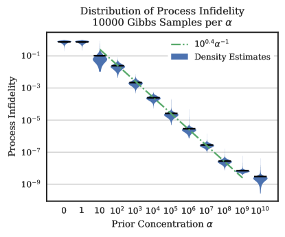
Figure 1: Violin plots showing distributions of process infidelity $1-f$ ($M=1000$ samples) drawn from $p_{\mu}(\xi;\alpha|I_{2}\rangle\rangle\langle\langle I_{2}|)$ The horizontal dashes indicate the means, and a regression fit for the means in the range $\alpha\in[10^{2},10^{8}]$ is superimposed. This illustrates a practical relationship between the concentration of the prior $\alpha$ and the average process infidelity of resulting random CPTP maps that can be used for setting informative priors, from e.g., RB. Furthermore, we conjecture that this trend persists beyond $\alpha=10^{8}$ if not for numerical precision issues.

Note that the increase in $\alpha$ scales roughly linearly with the process infidelity in the log-log scale for a wide range of infidelities. Furthermore, we suspect that this trend would continue for larger $\alpha$ if not for numerical issues, as $10^{-8}$ squared is approximately machine precision for 64 bit floating point numbers. Performing a regression on the transformed quantities, we arrive at $f\approx 1-10^{0.4}\alpha^{-1}$ which appears to be accurate for $\alpha\geq 100$, corresponding to a fidelity of roughly $0.97$. In other words, as the average of the distribution approaches the identity operation, the largest eigenvalue of the parameter matrix $\Theta$ must outscale the others and approach infinity, representing infinite concentration at the identity map.

The properties of frame-Bingham distribution imply that this eigenvalue scaling (and its impact on infidelity as a prior for fixed dimension $N$) holds for any target unitary operation since the particular target unitary only changes the eigenvectors of the $\Theta$ used, i.e., $\Theta=\alpha|U\rangle\langle U|$ for for an arbitrary unitary operation $U$. Furthermore, in the more general case of an average Choi matrix that does not correspond to a uniform depolarizing channel but is still “nearly” a unitary operation, the observed growth of the dominant eigenvector of $\Theta$ implies that the additional contributions due to the smaller eigenvalues is negligible. Thus, the single parameter prior $\Theta=\alpha|U\rangle\rangle\langle\langle U|$ will be a good choice for most practical applications.

IV.2 Bayesian Point Estimation

The maximum likelihood approach to estimation produces a so-called point estimate $\hat{\Lambda}_{MLE}$, whereas the Bayesian approach to estimation produces a probability distribution on $\Lambda$, as discussed above. Again, we reiterate that the mapping from $\xi$ to $\Lambda$ is measurable so $p_{\mu}$ and $p_{c}$ induce well defined distributions on the space of Choi matrices and thus we will be somewhat loose in applying these distributions to both cases. In the context of Bayesian estimation, two common approaches to producing point estimates are the maximum a posteriori (MAP) and expected a posteriori (EAP) estimators.

IV.2.1 MAP Estimation Using Exponential Families

The MAP approach defines a point estimator

$$\hat{\Lambda}_{MAP}=\operatorname*{arg\,max}_{\Lambda\textrm{ CPTP}}\,\,p(\Lambda|\mathbf{x},\mathbf{n})=\operatorname*{arg\,max}_{\Lambda\textrm{ CPTP}}\,\,p(\mathbf{x}|\Lambda,\mathbf{n})p(\Lambda),$$ (23)

since the normalizing term is constant in $\Lambda$ once $\mathbf{x}$ and the prior distribution have been fixed. Exponential family priors for MAP estimation have a special relationship with log-likelihood procedures for maximum likelihood estimation. Given an arbitrary exponential family prior for CPTP maps, recall that the functional form of such distribution would be

$$p_{exp}(\xi|\vartheta)=\exp(\langle\vartheta,T(\xi)\rangle-\psi(\vartheta))$$ (24)

where we have used $\vartheta$ to represent arbitrary natural parameters corresponding to some arbitrary sufficient statistics $T(\xi)$. Furthermore, we have expressed the exponential family as a distribution on the Stiefel manifold, but in principle exponential families defined for other representations of CPTP maps would apply to the discussion below. Using $p_{exp}$ as a prior results in a posterior distribution

$$p(\xi|\mathbf{x},\mathbf{n}) \propto p(\mathbf{x}|\xi,\mathbf{n})p_{exp}(\xi|\vartheta)$$ (25)

which is again an exponential family.

From a MAP estimation perspective,

$$\hat{\Lambda}_{MAP} =\Lambda\left(\operatorname*{arg\,max}_{\mathcal{\xi}}\,\,\log\left(p(\mathbf{x}|\xi,\mathbf{n})p_{exp}(\xi|\vartheta)\right)\right)$$ (26)

$$=\Lambda\left(\operatorname*{arg\,max}_{\xi}\,\,\log\left(p(\mathbf{x}|\xi,\mathbf{n})\right)+\langle\vartheta,T(\xi)\rangle\right).$$

Thus, the use of an exponential family prior can be applied to a log-likelihood based maximum likelihood estimation routine by adding the term $\langle(\vartheta,T(\xi)\rangle$. In particular, for our combined prior $p_{tot}(\xi;\Theta,\theta_{1},\theta_{2})$ we have

$$\hat{\Lambda}_{MAP}= \Lambda\bigg{(}\arg\max_{\xi}\,\,\log\left(p(\mathbf{x}+\theta_{1}|\xi,\mathbf{n}+\theta_{1}+\theta_{2})\right)$$ (27)

$$+\operatorname{Tr}\left(\Theta^{\dagger}\Lambda(\xi)\right)\bigg{)}$$

where setting $\Theta=0$ defines the uniform distribution on the Stiefel manifold, and the MAP estimate reduces to MLE estimate.

Since the prior $p_{c}$ folds in the binomial data in the likelihood this prior requires no changes to an existing maximum likelihood estimator. Indeed, this is equivalent to using conjugate priors on each tomographic experiment individually. The prior $p_{\mu}$ incorporates a single term in the log-likelihood estimator that is straight-forward to implement but obviously needs to be modified depending on the matrix representation used for the CPTP maps. This applies to Liouvillian superoperators through $\mathfrak{P}(\Theta)$ and for other linear transformations in an analogous manner. We have made these modifications to the gradient-based approach of Knee et al. (2018) which affects both the objective function, but also the rules for step size. Simulated results are shown in Section IV.2.3.

IV.2.2 EAP Estimation

The EAP estimate $\hat{\Lambda}_{EAP}$ is simply the mean of the posterior distribution, which to under an arbitrary prior with parameter $\vartheta$ is expressed as

$$\hat{\Lambda}_{EAP}=\int_{V_{N}(\mathbb{C}^{MN})}\Lambda(\xi)p(\xi|\mathbf{x},\mathbf{n},\vartheta)$$ (28)

This also has the interpretation of minimizing the mean squared error with respect to the posterior distribution. In other words, EAP estimates minimize the expected value of the loss function $L(\hat{\Lambda},\Lambda)=||\hat{\Lambda}-\Lambda||_{2}^{2}$. Other loss functions (i.e., different Bayes risks) can be used in an analogous fashion.

From a practical perspective, since the normalization constants in the posterior distribution for either prior $p_{\mu}$ and $p_{c}$ are intractable, this average is computed numerically using the Gibbs sampling routine. A sufficient number of samples from the posterior distribution $\{\xi^{(i)}\}\sim p(\xi|\mathbf{x},\mathbf{n},\Theta,\theta_{1},\theta_{2})$ are used to produce to produce an accurate average $\hat{\Lambda}=\frac{1}{|\{\xi^{(i)}\}|}\sum_{i}\Lambda(\xi^{(i)})$. Sampling from the posterior is more computationally intensive than the MLE or MAP approaches, and in our experience can have slow convergence and the potential for highly correlated samples, both of which require additional samples to be produced to maintain an effective sample size for an accurate estimate. That said, the production of EAP estimates generate approximations of the full posterior distribution allowing for the generation of credibility intervals as well as posterior distributions of other statistics, such as diamond norm (see Section IV.3).

IV.2.3 Simulation of Point Estimators

Simulated process tomography was performed using perfect state preparation and measurement for all combinations of the states $|0\rangle$, $|1\rangle$, $|+\rangle$ and $|-\rangle$. Ideal state preparation and measurement (SPAM) was used to clearly illustrate the impact of the prior on the estimation process without confounding factors. As maximum likelihood process tomography is a special case of the Bayesian approach presented here, the presence of SPAM errors should impact this Bayesian approach in much the same way as standard process tomography (see e.g., Merkel et al. (2013) for a brief discussion), but incorporation of prior information from SPAM agnostic procedures (such as RB) should bias the results towards the true fidelity. Incorporation of these priors into a self-consistent form of process tomography (such as GST Merkel et al. (2013); Blume-Kohout et al. (2016)) would address any concerns with SPAM errors and should be easily implemented for MAP estimates (see also Section V for additional discussion), and we leave this for future work. Each of the sixteen input/output combinations were repeated $n$ times varying over the set $\{10,10^{2},10^{3},10^{4},10^{5}\}$. Two sets of 100 ground truth CPTP maps were generated from $p_{\mu}(\xi;\alpha|I\rangle\rangle\langle\langle I|)$ with $\alpha=10^{2}$ and $10^{4}$, corresponding to average process fidelities of approximately $0.97$ and $0.9997$, respectively. These two priors, as well as the uniform $\alpha=0$ prior were used to perform MAP and EAP estimation. For the MAP estimates we used a slightly modified version of Knee et al. (2018), and note that the $\alpha=0$ prior corresponds to MLE. For the EAP estimates, 1000 burned in Gibbs samples from the sampler were used.

Figures 2 and 3 show the mean diamond norm error between the various point estimates and the two sets of ground truth maps used above. This is analogous to the root-mean-square error of the estimator. In accordance with general estimation theory, the estimators tend to converge to the true value as the number of measurements increases, and this this rate of decrease is eventually roughly proportional to the square root of the number of measurements. These figures also demonstrate how the priors interact with the data, in that an informative prior can bias the estimate and result in a more accurate estimate given fewer measurements (Fig. 3), but can also bias the estimate in a negative manner when the true map is unlikely given a highly concentrated prior (Fig. 2). Additionally, it appears that the diffuse prior cases in Fig. 3 are suffering reduced effective sample size, since the EAP estimates diverge slightly from the MAP estimates as the sample sizes increase. This issue is is really only a problem in the automated analysis here, for analysis of a single experiment, visual inspection of the samples or other methods for estimating effective sample size could be employed.

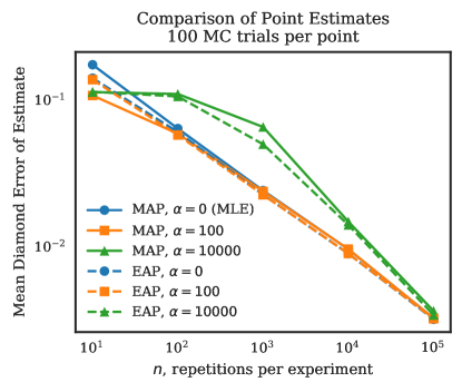
Figure 2: Comparison of mean diamond error to ground truth for different combinations of estimators (MLE, MAP, and EAP) and priors (defined by parameter $\alpha|I\rangle\rangle\langle\langle I|$). Ground truth gates were drawn from the distribution $p_{\mu}(\xi;\alpha|I\rangle\rangle\langle\langle I|)$ with $\alpha=100$, which corresponds to an average process fidelity of $\approx 0.97$. The priors correspond to average process fidelities of $0.25$, $\approx 0.97$ and $\approx 0.9997$ for $\alpha=0$, $100$, and $10000$, respectively. The Bayesian estimates with the correct ($\alpha=100$) prior produce slight improvements over MLE but due to the relative weakness of the prior this advantage is quickly erased with increasing $n$. The prior with $\alpha=10000$ is highly concentrated and it requires considerable data to overcome this mismatched prior, as the ground truth samples are highly unlikely for this prior.

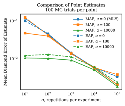
Figure 3: Comparison of mean diamond error to ground truth for the same combination of estimators and priors as Fig. 2. Here, however, ground truth gates were drawn from the prior $p_{\mu}(\xi;\alpha|I\rangle\rangle\langle\langle I|)$ with $\alpha=10000$, which corresponds to an average process fidelity of $\approx 0.9997$. Given the high concentration of the ground truth distribution the advantages of the matched prior are shown with substantial improvement in estimation error for small $n$. We believe the divergence in the EAP estimators for $n=10^{5}$ is likely due to occasional poor convergence in the underlying MCMC samples which can be avoided via manual inspection (to continue to produce samples) but is difficult to avoid in an automated fashion.

Figures 2 and 3 focused on the overall estimation error between the tomographic reconstruction and the true map. Since the prior $p_{\mu}$ is specified in terms of average process fidelity, analyzing the behavior of the estimators with respect to process fidelity offers an alternative view to the properties of the estimators. Figures 4 and 5 show the mean process infidelity of the estimators as a function of $n$. As we expect from the Figs. 2 and 3 the process infidelities converge across all estimators as $n$ increases. These figures indicate that MAP and MLE estimation will produce higher estimates of process fidelity than EAP estimation using the uniformly depolarizing prior considered here. In particular, EAP estimates with a properly matched prior produce the most accurate estimates of process infidelity. This discrepancy between the estimated infidelity despite the similarity in overall diamond error indicates that the MAP (and MLE) approaches are heavily biased towards the dominant eigenvectors of the prior parameter as compared with EAP estimation.

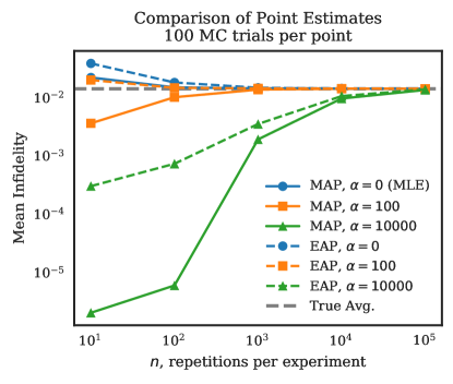
Figure 4: Comparison of mean process infidelity to the identity map for the same combinations of estimators and priors as Fig. 2, as well as the sample average of the process infidelities of the ground truth gates. Ground truth gates were drawn from the prior $p_{\mu}(\xi;\alpha|I\rangle\rangle\langle\langle I|)$ with $\alpha=100$ corresponding to an average process fidelity of $\approx 0.97$. As expected, the MAP estimates are highly biased with respect to the process infidelity, as compared with the EAP estimates, and the EAP estimates with $\alpha=100$ produce the closest posterior infidelities to the truth data. Note, however, that despite large deviations in the process infidelity of the estimates, the diamond errors between the estimates and true gates are similar (see Fig. 2).

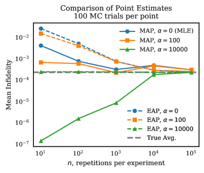
Figure 5: Comparison of mean process infidelity to the identity map for the same combinations of estimators and priors as Fig. 2, as well as the sample average of the process infidelities of the ground truth gates. Ground truth gates were drawn from the prior $p_{\mu}(\xi;\alpha|I\rangle\rangle\langle\langle I|)$ with $\alpha=10000$ corresponding to an average process fidelity of approximately $0.9997$. The trends here are essentially the same as Fig. 4, but even more pronounced.

IV.3 Posterior Distributions and Credibility Intervals

In addition to point estimation, the Gibbs sampling routine from the posterior distribution can be used for additional Bayesian approaches such as the construction of credibility intervals. As an example, Fig. 6 shows histograms of posterior distributions for different combinations of prior and $\mathbf{n}$, along with the inner 95 percentile of the posterior distribution, i.e., the 95% credibility interval. The two upper left panel shows the uniform prior with $n_{i}=100$ measurements per state preparation and measurement configuration, the upper right the uniform prior with $n_{i}=10^{5}$, the lower left the prior $p_{\mu}(\xi;10^{4}|I\rangle\rangle\langle\langle I|)$ with $n_{i}=100$, and the bottom left panel the prior $p_{\mu}(\xi;10^{4}|I\rangle\rangle\langle\langle I|)$ and $n_{i}=10^{5}$.

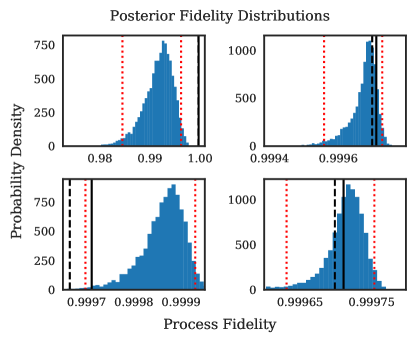
Figure 6: Comparison of posterior distributions. Each subfigure corresponds to 10000 samples from the posterior distribution. Top row: Uniform priors. Bottom row: prior $p_{\mu}(\xi;10^{4}|I\rangle\rangle\langle\langle I|)$. Left column $n_{i}=100$ measurements per simulated experiment. Right column $n_{i}=10^{5}$ measurements per simulated experiment. Black solid line indicates the true process fidelity, the dashed black line the fidelity of the MLE. Red dotted lines denote the inner 95% credibility interval determined by the posterior samples.

Samples from the posterior distributions can also be used to perform Bayesian analysis of arbitrary functions of the posterior distribution of CPTP maps. As an example, Fig. 7 shows posterior distributions of the diamond error (from the identity map) for the same data shown in Fig. 6. This shouldn’t be confused with data shown in Figs. 2 and 3 which show the diamond error between the point estimates and the true gates across an ensemble of simulated tomography experiments. The plots on the left illustrate the strength of the prior in terms of its concentration in diamond norm. The uniform prior for the $n_{i}=100$ case is considerably less concentrated than for the $\alpha=10^{4}$ prior. Additionally, since the true map was drawn from the $\alpha=10^{4}$ prior, the true diamond error is in the 95% posterior credibility interval for the bottom-left plot, but not when the uniform prior is used. However, when $n_{i}$ is large (corresponding to the right column) the posterior distributions (and resulting credibility intervals) are much closer.

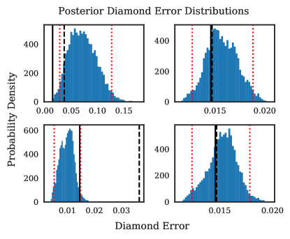
Figure 7: Comparison of posterior distributions of diamond error. Each subfigure corresponds to 10000 samples from the posterior distribution (the same samples as Fig. 7). Top row: Uniform priors. Bottom row: prior $p_{\mu}(\xi;10^{4}|I\rangle\rangle\langle\langle I|)$. Left column $n_{i}=100$ measurements per simulated experiment. Right column $n_{i}=10^{5}$ measurements per simulated experiment. Black solid line indicates the true process fidelity, the dashed black line the fidelity of the MLE. Red dotted lines denote the inner 95% credibility interval determined by the posterior samples. These plots highlight the power of a posterior distribution, as we can produce estimates and credibility intervals of functions of the underlying quantum process that are otherwise experimentally inaccessible.

V Conclusion

In this work we have used the theory of exponential families of probability distributions using Stiefel manifolds as a sample space to induce distributions on the space of CPTP maps. These distributions are used in Bayesian analysis of process tomography as both prior and posterior distributions. From the perspective of priors, one of these distributions is the maximum entropy distribution defined by an average Choi matrix, whereas the other is equivalent to the conjugate prior for the binomial distributions that underlie process tomography experiments. We compared Bayesian MAP and EAP point estimators and discussed some impacts of the priors on the estimators. Additionally, we showed that the Gibbs sampling approach can be used to produce posterior credibility intervals for parameters of interest.

The analysis and examples presented in this manuscript are by no means exhaustive, the primary focus was on demonstrating that the priors and sampling approaches work correctly, and that the results agree with the general theory of Bayesian estimation in a classical context. In particular, for the full Bayesian analysis, we only considered some basic parameters of CPTP maps, one could envision other parameters of interest such as nonunitarity (i.e., translation of the center of the Bloch sphere via the CPTP map). Another aspect of Bayesian estimation which we have not touched are sequential techniques. The distributions discussed here could be used as proposal distributions for the techniques proposed in Granade et al. (2016); Pogorelov et al. (2017).

As far as future extensions, we note that we have already shown how the method of Hoff (2009) can be extended to include essentially arbitrary functions of a CPTP map (here we used $\log$). This observation allows for the definition and sampling of a wide range of distributions on the space of CPTP maps. For example, the addition of regularizers or penalty terms to a maximum likelihood estimation process can often be interpreted in Bayesian context as the component due to a particular choice of (exponential family) prior in a MAP process Seeger and Wipf (2010); Stuart (2010). Thus sparsity-enforcing regularization terms used for process tomography (e.g., an $\ell_{1}$ penalizer as in Mohseni et al. (2008)) can be interpreted as MAP estimates using an exponential family. Considering $||\Lambda||^{2}_{2}$ or $||\Lambda||_{1}$ as parameters in an exponential family (perhaps expressed in a Pauli Basis) appear to be implementable in the Gibbs sampling framework, and thus the use of these sorts of regularization terms can be analyzed in the fully Bayesian context. Many other natural quantities of interest can be expressed as simple functions of $\Lambda$, and thus can be interpreted in the framework of exponential families on Stiefel manifolds.

The other major extension that we see for these concepts is to define joint distributions between CPTP maps. In one sense, since $\exp$ and the Gibbs sampling framework naturally factorizes, the algorithm can be extended to add another layer of conditional sampling. However, for more complex tomographic procedures such as gate set tomography Merkel et al. (2013); Blume-Kohout et al. (2016), the likelihood terms will be higher order polynomials in the random gates and will likely require clever handling in the inner loops of the sampling routine to remain computationally tractable.

Aside from the applications of these distributions to process tomography we note that these distributions could also be applied to circuit simulation to study the effects of non-Pauli errors in circuit simulation and threshold computations. Related to this, we note that a future direction of research is the distribution on quantum states induced by the application of these random CPTP maps to a given input state. Furthermore, it should be possible to introduce correlations between errors and use a similar Gibbs sampling approach to generate random errors that are correlated in both time and space.

Appendix A Sampling Algorithm

The algorithm of Hoff (2009) uses several stages of Markov Chain Monte Carlo (MCMC) sampling to generate random samples whose stationary distribution converges to the target distribution. As noted in the main text, the algorithm is designed for real-valued Stiefel manifolds, so we use the procedure in Kent et al. (2013) to convert between $V_{N}(\mathbb{C}^{MN})$ to $V_{N}(\mathbb{R}^{2MN})$. The outermost layer of sampling produces a new sample $\xi^{\prime}$ from the current sample $\xi$. Inside this layer, the next layer selects a column $r$ and then $\xi_{r}$ is generated conditionally with the remaining columns (denoted $\xi_{-r}$). This process is repeated for a random permutation of $\{1,\dots,N\}$ so that all columns are sampled, resulting in a new sample $\xi^{\prime}$. To sample a column $\xi_{r}$ conditioned on $\xi_{-r}$, let $z=\mathcal{N}^{\dagger}\xi_{r}$, with $\mathcal{N}$ and orthonormal basis for the null space of $\xi_{-r}$. The final MCMC stage then samples the coordinates $z_{i}$ in random order conditioned on the remaining parameters, denoted $z_{-i}$. These steps are summarized in Algorithm 1, with the further detail and derivation of the underlying distributions following.

Algorithm 1 Sampling $p(\xi^{\prime}|\xi)$

function OuterMCMCStep($\xi,\Theta,\{A_{j}\},\mathbf{x},\mathbf{n}$)

     for $r$ in randperm$(\{1,\dots,N\})$ do

         $\mathcal{N}\leftarrow I-\xi_{r}\xi_{r}^{\dagger}$

         $z\leftarrow\mathcal{N}^{\dagger}\xi_{r}$

         for $i$ in randperm$(\{1,\dots,2MN-1\}$ do

              $\tau\leftarrow z_{i}^{2}$

              $s\leftarrow\texttt{sign}(z)$

              $q_{-i}\leftarrow z_{-i}^{2}/(1-\tau)$

              Sample $\tau^{\prime}\propto p(\tau^{\prime},1|q_{-i},s_{-i})+p(t,-1|q_{-i},s_{-i})$

              Sample $s^{\prime}\propto p(\tau^{\prime},s^{\prime}|q_{-i},s_{-i})+p(\tau^{\prime},s^{\prime}|q_{-i},s_{-i})$

              $z\leftarrow\frac{\sqrt{1-\tau^{\prime}}}{\sqrt{1-\tau}}z$

              $z_{i}\leftarrow\sqrt{\tau^{\prime}}s$

         end for

         $\xi_{r}\leftarrow\mathcal{N}z$

     end for

     return $\xi$

end function

From the above algorithm, one can see that the true difficulty lies in sampling $\tau^{\prime}$ and $s^{\prime}$, with the remainder of the algorithm being an exercise in linear algebra. The conditional posterior distribution of the column $\xi_{r}$ (without loss of generality we ignore $\theta_{1}$ and $\theta_{2}$) is given by

$$p(\xi_{r}|\xi_{-r},\Theta,\mathbf{x},\mathbf{n})\propto\exp\Biggl{(}\xi_{r}^{\dagger}(\Theta\otimes I_{M})_{[r,r]}\xi_{r}\\ +2\operatorname{Re}\biggl{(}\sum_{j\neq r}\xi_{j}^{\dagger}(\Theta\otimes I_{M})_{[j,r]}\xi_{r}\biggr{)}\\ +\sum_{j=1}^{m}x_{j}\log\Biggl{[}\xi_{r}^{\dagger}(A_{j}\otimes I_{M})_{[r,r]}\xi_{r}\\ +2\operatorname{Re}\biggl{(}\sum_{k\neq r}\xi_{k}^{\dagger}(A_{j}\otimes I_{M})_{[k,r]}\xi_{r}\biggr{)}+\sum_{k\neq r}\xi_{k}^{\dagger}(A_{j}\otimes I_{M})_{[k,k]}\xi_{k}\Biggr{]}\\ +\sum_{j=1}^{m}(n_{j}-x_{j})\log\Biggl{[}1-\xi_{r}^{\dagger}(A_{j}\otimes I_{M})_{[r,r]}\xi_{r}\\ -2\operatorname{Re}\biggl{(}\sum_{k\neq r}\xi_{k}^{\dagger}(A_{j}\otimes I_{M})_{[k,r]}\xi_{r}\biggr{)}-\sum_{k\neq r}\xi_{k}^{\dagger}(A_{j}\otimes I_{M})_{[k,k]}\xi_{k}\Biggr{]}\Biggr{)}\,.\\$$ (29)

Applying the substitution $z=\mathcal{N}^{\dagger}\xi_{r}$ and gathering like terms, the conditional posterior distribution of an element $z_{i}$ given the remaining elements $z_{-i}$ (and $\xi_{-r}$, etc.,) is

$$p(z_{i}|z_{i-1},\dots)\propto\exp\biggl{(}bz_{i}^{2}+z_{-i}^{\dagger}Bz_{i}+2\operatorname{Re}(c_{i}^{\dagger}z_{i}+c_{-i}^{\dagger}z_{-i})\\ +\sum_{j=1}^{m}x_{j}\log\biggl{[}\tilde{b}_{j}z_{i}^{2}+z_{-i}^{\dagger}\tilde{B}_{j}z_{-i}\\ +2\operatorname{Re}((\tilde{c}_{j})^{\dagger}_{i}z_{i}+(\tilde{c}_{j})^{\dagger}_{-i}z_{-i})+\tilde{d}_{j}\biggr{]}\\ +\sum_{j=1}^{m}(n_{j}-x_{j})\log\biggl{[}1-\tilde{b}_{j}z_{i}^{2}-z_{-i}^{\dagger}\tilde{B}_{j}z_{-i}\\ -2\operatorname{Re}((\tilde{c}_{j})^{\dagger}_{i}z_{i}+(\tilde{c}_{j})^{\dagger}_{-i}z_{-i})-\tilde{d}_{j})\biggr{]}\biggr{)},\\$$ (30)

where the terms $b$, $\tilde{b}_{j}$, and $d_{j}$ are scalars, $c$ and $\tilde{c}_{j}$ are vectors, and $B$ and $\tilde{B}_{j}$ are matrices whose straightforward computation from $\mathcal{N}$, $\Theta$, $A_{i}$, and $\xi_{j}$ we have omitted.

As in Hoff (2009) we perform yet another coordinate transformation, letting $\tau=z_{i}^{2}$, $s_{i}=\operatorname{sign}(z_{i})$, $q_{-i}=z^{2}_{-i}/(1-\tau)$ where the exponent here is elementwise, and $s_{-i}=\operatorname{sign}(z_{-i})$, a vector of signs. Thus, $z_{i}=\sqrt{\tau}s_{i}$ and $z_{-i}=\sqrt{1-\tau}\sqrt{q_{-i}}\circ s_{-i}$ where $\sqrt{\cdot}$ is elementwise and $\circ$ denotes elementwise multiplication. Applying the chain rule as in (Hoff, 2009, Sec. 3.1) yields an expression for the joint distribution of $\tau$ and $s_{i}$ as

$$p(\tau,s_{i}|q_{-i},s_{-i},\dots)\propto\\ p(z_{i}=\sqrt{\tau}s_{i}|z_{-i}=\sqrt{1-\tau}q_{-i}\circ s_{-i},\dots)\\ \times\tau^{-\frac{1}{2}}(1-\tau)^{\frac{(NM-4)}{2}}\,.$$ (31)

Sampling $z_{i}$ then amounts to sampling $\tau$ from

$$p(\tau,s_{i}=1|q_{-i},s_{-i})+p(\tau,s_{i}=-1|q_{-i},s_{-i})$$ (32)

and then sampling $s_{i}$ given the chosen $\tau$. We found that the distributions of interest here are often too strongly concentrated to use the rejection sampling approach in Hoff (2009). Instead, we adopt the other suggestion in Hoff (2009), using a grid-based sampling of $\tau$. The gist of the approach is to start with an initial sample of $K$ evenly spaced $\tau_{j}$ from $(0,1)$, evaluate their probabilities, and sample nearby points whose probabilities are within some threshold of the maximum sampled probability. This process is repeated, retaining only the likely samples until an effective sample size criteria is reached. Here we used a standard criterion from the field of sequential Monte Carlo Doucet et al. (2001), and set the effective sample size to $K_{eff}=(\sum w_{j}^{2})^{-1}$, where $w_{j}$ are the normalized weights of the samples $\tau$. Here, the adaptive sampling procedure was terminated when $K_{eff}\geq K_{min}=K/10$. This process is described in Algorithm 2. Once the sampling of $\tau$ has been completed, sampling of $s_{i}$ is done using the distribution defined by $p(s_{i}|\tau,\dot{)}$ for $s_{i}\pm 1$. Cycling through Algorithm 1 for all columns will then result in a new sample for $\xi$.

Algorithm 2 Adaptive Grid Sampling of $\tau$

$K_{eff}\leftarrow K_{min}-1$

$T\leftarrow$ linspace$(0,1,K)$

$\Delta\leftarrow 1/K$

for $\tau_{j}\in T$ do

     $p_{j}\leftarrow p(\tau_{j},s_{i}=1|q_{-i},s_{-i})+p(\tau_{j},s_{i}=-1|q_{-i},s_{-i})$

     $w_{j}\leftarrow p_{j}/\sum p_{j}$

end for

$K_{eff}=(\sum p_{j}^{2})^{-1}$

while $K_{eff}<K_{min}$ do

     $\Delta\leftarrow\Delta/K$

     $T^{\prime}\leftarrow\{\}$

     for $\tau_{j}\in T$ do

         if $w_{j}>\varepsilon\max_{j}{w_{j}}$ then

              $T^{\prime}=T^{\prime}\cup$linspace$(\tau_{i}-\frac{\Delta}{2},\tau_{j}+\frac{\Delta}{2},K)$

         end if

     end for

     $T\leftarrow T^{\prime}$

     for $\tau_{j}\in T$ do

         $p_{j}\leftarrow p(\tau_{j},s_{i}=1|q_{-i},s_{-i})+p(\tau_{j},s_{i}=-1|q_{-i},s_{-i})$

         $w_{j}\leftarrow p_{j}/\sum p_{j}$

     end for

     $K_{eff}=(\sum p_{j}^{2})^{-1}$

end while

Sample $\tau$ from $p(\tau_{j})=w_{j}$

In the simple tomography experiments considered here, the terms in Eq. (32) due to the binomial distribution can be computed rapidly for a set of candidate $\tau_{j}$ using the vectorization and broadcasting capabilities of modern computer linear algebra package. This is possible because the terms in Eq. 30 can be expressed in relatively simple terms once the portions dependent on the other columns $\xi_{-r}$ are fixed. In a more complex tomographic experiment such as gate set tomography, the likelihood expressions of the resulting binomial distributions will depend on several elements from Stiefel manifolds (one for each gate), and while the joint family will still be an exponential family, the expressions for the likelihood will likely be more complicated and considerable thought will be required to make sampling from the grid efficient.