Classical properties of the leading eigenstates of quantum dissipative systems

Abstract

By analyzing a paradigmatic example of the theory of dissipative systems – the classical and quantum dissipative standard map – we are able to explain the main features of the decay to the quantum equilibrium state. The classical isoperiodic stable structures typically present in the parameter space of these kind of systems play a fundamental role. In fact, we have found that the period of stable structures that are near in this space determines the phase of the leading eigenstates of the corresponding quantum superoperator. Moreover, the eigenvectors show a strong localization on the corresponding periodic orbits (limit cycles). We show that this sort of scarring phenomenon (an established property of Hamiltonian and projectively open systems) is present in the dissipative case and it is of extreme simplicity.

I Introduction

Open quantum systems have received great attention recently Weiss . One of the main reasons has been the development of quantum information and computation Nielsen ; Preskill , but also the experiments with cold atoms CAexp ; AOKR , and Bose-Einstein condensates BEC can significantly profit from their study. The engineering of reservoirs has been applied to generate robust quantum states in the presence of decoherence Kienzler , providing with a new perspective in our study of quantum environments. The route to chaos that is a typical feature of dissipative systems has recently been studied in optomechanics Bakemeier . The interest has also been focused on many body systems Hartmann . In this case the study of the rocked open Bose-Hubbard dimer has revealed the connection between the interactions and bifurcations in the mean field dynamics. Very recently, quantum bifurcation diagrams have been obtained Ivanchenko . In all these established and promising areas the properties of the leading eigenstates of the associated quantum superoperators are of the utmost relevance, but have not been deeply investigated.

Up to now, the spectral behaviour of quantum dissipative systems has been characterized by means of a Weyl law Spina whose theoretical explanation is still more elusive than the one for the usual fractal Weyl law for projectively open systems. On the other hand, asymptotic states associated to an eigenvalue $\lambda_{0}=1$ have been investigated in a system that is of interest in directed transport studies, the dissipative modified kicked rotator map Carlo ; Beims . However, the results obtained can be assumed to be of general nature and thus applicable to any kind of dissipative system. There, the fundamental role played by the so called isoperiodic stable structures (ISSs) of the classical system has been investigated. In particular it was conjectured that their quantum counterparts (qISSs) have the simple shape of the ISSs only for exceptionally large regular structures. In the majority of the cases qISSs look approximately the same as the quantum chaotic attractors that are at their vicinity in parameter space Carloprl . This conjecture was proven in Carlo by means of a systematic exploration of the quantum parameter space, showing how sharp classical borders become blurred and neighboring areas influence each other through quantum fluctuations. This phenomenon was called parametrical tunneling.

We here investigate the other aspect of this phenomenon, that is, how the presence of an ISS, even if not visible in the smooth quantum parameter space, manifests itself in the quantum dynamics. We focus on the properties of the leading eigenstates. These states , about which little is known, are very important since they rule the transitory behaviour, i.e. the way the system decays towards the equilibrium. It turns out that their phase space structure as well as the phase of their corresponding eigenvalues can be related to the shape and periodicity of a neighbouring ISS, respectively. The corresponding limit cycles not only influence the quantum system at the parameter values at which they appear classically, but also at their neighbourhood. This leads to localization on unstable periodic orbits. Hence, this phenomenon ubiquitous in the quantum chaos literature dealing with Hamiltonian systems, and also in the optics area that treats projectively open resonators scarring , is also present in the dissipative arena, adopting a very simple behaviour.

For our calculations we choose a paradigmatic case of dissipative dynamics: the classical and quantum dissipative standard map (DSM). The corresponding parameter space (in the parameter range we are considering) consists of a large regular region and a chaotic sea where regular structures are embedded.

We explain the details of the classical and quantum dissipative standard map in Sec. II, together with the techniques used to study their properties. In Sec. III we present our results focusing on the details of the parameter space and taking special care of the Husimi representations of the eigenvectors associated to the leading eigenstates. We close with Sec. IV where we state our conclusions.

II The dissipative standard map: calculation methods

The standard map can be thought of as describing the dynamics of a particle moving in a coordinate $x$ with [$x\in(-\infty,+\infty)$] that is periodically kicked by the single harmonic potential:

$$V(x,t)=k\left[\cos(x)\right]\sum_{m=-\infty}^{+\infty}\delta(t-m\tau),$$ (1)

where $k$ is the strength of these kicks and $\tau$ is the period. Dissipation can be added to obtain the DSM Schmidt

$$\left\{\begin{array}[]{l}\overline{n}=\gamma n+k[\sin(x)]\\ \overline{x}=x+\tau\overline{n}.\end{array}\right.$$ (2)

We take $n$ as the momentum variable conjugated to $x$ and $\gamma$ ($0\leq\gamma\leq 1$) is the dissipation parameter. By varying it the map performs a transition from the Hamiltonian standard map ($\gamma=1$) to the one-dimensional circle map ($\gamma=0$). We can define a rescaled momentum variable $p=\tau n$ and the quantity $K=k\tau$ in order to simplify things.

This map can be easily quantized by taking: $x\to\hat{x}$, $n\to\hat{n}=-i(d/dx)$ ($\hbar=1$). Since $[\hat{x},\hat{p}]=i\tau$ (where $\hat{p}=\tau\hat{n}$), the effective Planck constant is $\hbar_{\rm eff}=\tau$. In order to reach the classical limit $\hbar_{\rm eff}\to 0$, while $K=\hbar_{\rm eff}k$ remains constant. We have taken $\hbar_{\rm eff}=0.042$, i.e. a finite value. Quantum dissipation leads us to a master equation Lindblad for the density operator $\hat{\rho}$ in such a way that

$$\dot{\hat{\rho}}=-i[\hat{H}_{s},\hat{\rho}]-\frac{1}{2}\sum_{\mu=1}^{2}\{\hat{L}_{\mu}^{{\dagger}}\hat{L}_{\mu},\hat{\rho}\}+\sum_{\mu=1}^{2}\hat{L}_{\mu}\hat{\rho}\hat{L}_{\mu}^{{\dagger}}\equiv\Lambda\rho.$$ (3)

Here $\hat{H}_{s}=\hat{n}^{2}/2+V(\hat{x},t)$ is the system Hamiltonian, { , } is the anticommutator, and $\hat{L}_{\mu}$ are the Lindblad operators given by Dittrich ; Graham

$$\begin{array}[]{l}\hat{L}_{1}=g\sum_{n}\sqrt{n+1}\;|n\rangle\,\langle n+1|,\\ \hat{L}_{2}=g\sum_{n}\sqrt{n+1}\;|-n\rangle\,\langle-n-1|,\end{array}$$ (4)

with $n=0,1,...$ and $g=\sqrt{-\ln\gamma}$ (to comply with the Ehrenfest theorem).

In order to perform the classical evolution we directly use the map of Eq. 2. In some cases, for comparison purposes, we will be interested in a coarse grained version of the exact dynamics UlamDMaps . For this we will use the Ulam method Ulam which is an approximation to the Perron-Frobenius operator arising from the Liouville equation for the the map in Eq. 2, obtained by discretizing the phase space.

In the quantum case we numerically integrate Eq. 3 and obtain the evolution of the density matrix (symbolically) as $\rho_{t+1}=e^{\Lambda}\rho_{t}$, where $e^{\Lambda}$ is a non-unital superoperator of dimension $N^{2}\times N^{2}$. The effective Planck size is given by $\hbar_{\rm eff}\propto{1/N}$. Classical and quantum dissipation provides with a natural bound that allows for the truncation of the phase space, leaving all the relevant dynamics inside of the resulting domain, and providing with finite (super)operators. The diagonalization of the Ulam superoperator and of the quantum $e^{\Lambda}$, is performed by the Arnoldi method Arnoldi .

III Properties of the leading eigenstates: the decay towards equilibrium

In order to characterize the behaviour of the leading eigenstates of the DSM we need first to explore the parameter space spanned by $k$ and $\gamma$. For that purpose we calculate the participation ratio defined by $\eta=(\sum_{i}P(p_{i})^{2})^{-1}/N$. $P(p_{i})$ is a discretized limiting momentum ($p$) distribution, taken after evolving $10000$ time steps a bunch of $10000$ random initial conditions in the $p=[-k/(1-\gamma);k/(1-\gamma)]$ band of the cylindrical phase space (i.e., the trapping region defined in Martins ). We have taken a number of bins given by a Hilbert space dimension $N=1000$. Taking a finer coarse-graining would not affect the main properties in which we are interested since the distance among points of the simple limit cycles is always greater than the bin size. This measure is a good indicator of the complexity of the asymptotic distribution. It is worth mentioning that the DSM contains multistability regions with a great number of coexisting attractors Martins . However, we are interested in clearly identifying those regions where just regular behavior is found and those where a chaotic attractor is present. For this objective our measure is a very suitable one. Results are shown in Fig. 1 a).

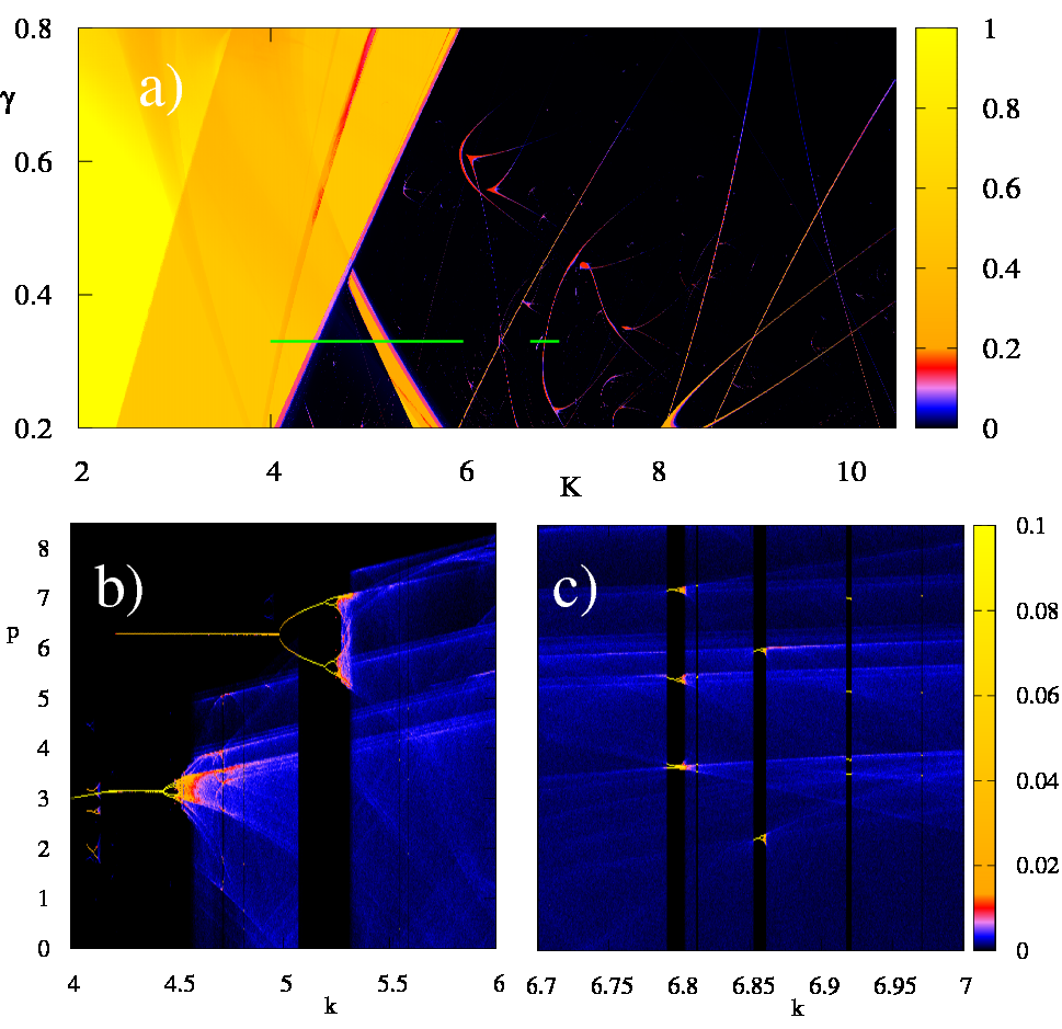
Figure 1: (color online) Top panel $a)$ shows the participation ratio $\eta$ vs. parameters $k$ and $\gamma$ (for details see main text). Bottom panels $b)$ and $c)$ illustrate probability in momentum $P(p)$ as a function of $k$ for $\gamma=0.33$ corresponding to the ranges shown in green lines in panel $a)$.

The diagonal line that can be clearly seen in this figure corresponds to the onset of chaotic behavior. On the right side of this line, in general tiny “regular islands” (where only regular behaviour is present) can be found within the “chaotic sea”. These are the previously mentioned ISSs, i.e. Lyapunov stable islands that come organized into families in the parameter space, which usually have long antenna like branches leading to nicknaming them as “shrimps”.

The bifurcations diagrams along a line with fixed dissipation parameter $\gamma=0.33$ and $k$ in the intervals $4.0\leq k\leq 6.0$ (Region 1) and $6.7\leq k\leq 7.0$ (Region 2) are shown in panels b) and c) of Fig. 1 (we display the probability in momentum $P(p)$ as a function of $k$). They complement Fig. 1 a) by providing information on the limit cycles which characterize the selected regular regions.

We first present the results of the diagonalization of the quantum superoperator $e^{\Lambda}$ with an effective $\hbar_{\rm eff}=0.042$ for four representative points of Region 1. Case a) corresponds to ($\gamma=0.33,k=4.0$) located in the regular region, case b) to ($\gamma=0.33,k=5.13$) in the interior of the largest regular island found in the explored parameter space. The two other points belong to the chaotic set: ($\gamma=0.33,k=5.5$) (case c) ) is in the vicinity of the island, while ($\gamma=0.33,k=6.0$) (case d) ) lies in a region where no islands are visible at our resolution. Fig. 2 shows the eigenvalue spectra in complex space for these four cases. The corresponding Husimi representations of the invariant state (left panels) and of the leading eigenstate (right panels) are displayed in Fig. 3.

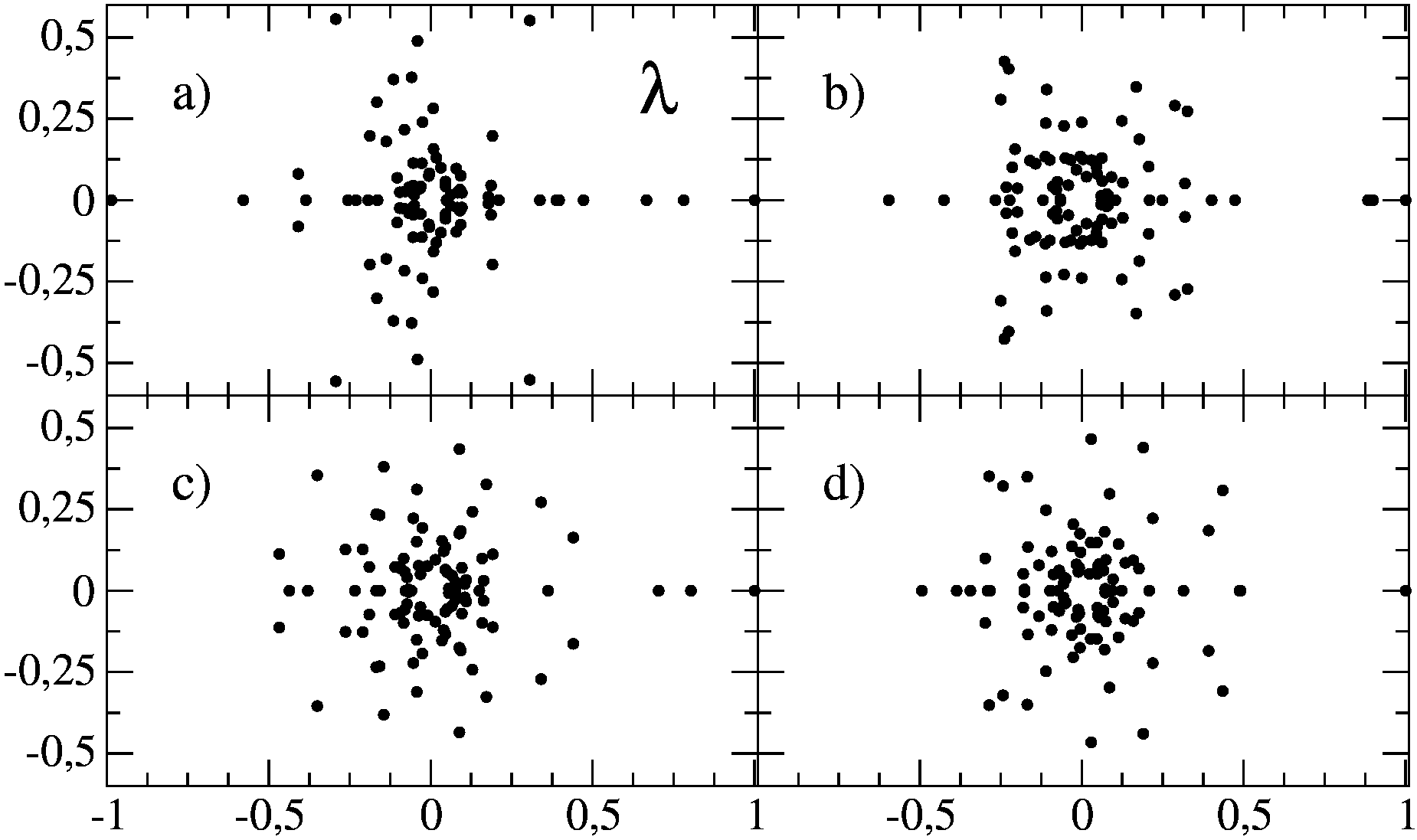
Figure 2: 100 largest eigenvalues of the quantum superoperator $e^{\Lambda}$ for a) ($\gamma=0.33,k=4.0$), b) ($\gamma=0.33,k=5.13$), c) ($\gamma=0.33,k=5.5$), d) ($\gamma=0.33,k=6.0$). $\hbar_{\rm eff}=0.042$.

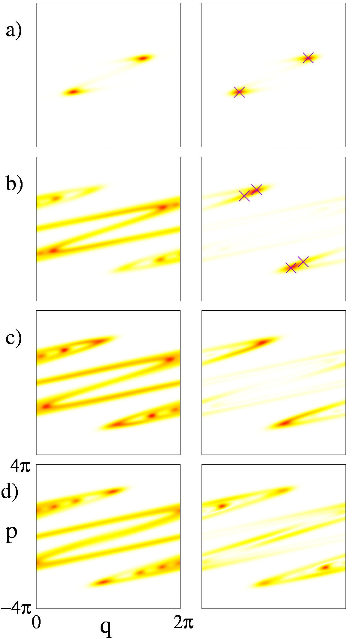
Figure 3: (color online) Husimi representation of the invariant state (left panel) and leading eigenstate (right panel) for a) ($\gamma=0.33,k=4.0$), b) ($\gamma=0.33,k=5.13$), c) ($\gamma=0.33,k=5.5$), d) ($\gamma=0.33,k=6.0$). $\hbar_{\rm eff}=0.042$. In the right panels of a) and b) the periodic points of the ISSs are marked with crosses.

The invariant state shown in 3 a) for parameters deep inside the regular region exhibits a point like structure which coincides, within quantum uncertainty, with a stable periodic orbit with winding number $0/2$. This orbit has been calculated with the method proposed in wenzel and is marked with crosses. It corresponds to the period two limit cycle which is visible in the bifurcation diagram of Fig. 1 b). The leading resonance with $\lambda_{1}=-0.985733$ shown in the right panel of Fig. 3 a) presents a very similar point-like distribution. Moreover we have verified that all states corresponding to eigenvalues close to the unit circle in the spectrum of Fig. 2 a) have a simple structure. For real eigenvalues the Husimi distributions look very much the same as the one of Fig. 3 a) while for the largest complex eigenvalues which have phases approximately equal to multiples of $\pi/3$ they are peaked on a period three limit cycle also present in this region (see Fig.1 b)). As we go to lower eigenvalues of the spectrum all point-like eigenstates get more and more blurred. These results confirm that in the regular region of the parameter space quantum dynamics reproduces (within quantum uncertainty) the main features of the classical one.

This is not the case for parameters belonging to an ISS. As shown in Fig.3 b) the invariant state does not follow the asymptotic classical distribution characterized by a period two limit cycle, but has instead the complex structure of a strange attractor. In fact, it looks very much the same as the states obtained in the chaotic region which are shown in the two panels below. This is an indication that in what regards the equilibrium states the ISS cannot be resolved at our value of $\hbar_{\rm eff}$. However the situation is different if we look at the leading eigenstate shown in the right panel of Fig.3 b). Its Husimi distribution is strongly localized on a periodic orbit with winding number $2/2$ marked by crosses in this Figure. The corresponding eigenvalue is real and large ( $\lambda_{1}\sim 0.9$ ) as we can see from the spectrum of Fig.2 b), hinting at a long decay time towards the complex invariant state. The following states are significantly shorter lived ($|\lambda_{1}|\sim 0.6$) and even if they show some localization on orbits present in the island, they essentially have the structure of the attractor.

We obtain analogous results for parameters which do not belong to the ISS but are close to it. As expected, the equilibrium state shown in Fig.3 c) is a complex attractor, this time in agreement with the asymptotic classical distribution. However, as in the previous case, the presence of the regular island influences the leading eigenstate. Even if the distribution shown in the right panel of Fig.3 c) is not strictly point-like it still has a clearly enhanced probability on the periodic orbit $2/2$ which is unstable now. In fact, the enhancement of probability on an unstable periodic orbit is the definition of scarring. The corresponding eigenvalue $\lambda_{1}=0.8$ is real and fairly large, indicating a long transient also in this case. The spectrum in Fig.2 c) shows the existence of a second real eigenvalue $\sim 0.7$ considerably larger than the radius of the dense disk. It corresponds to a state with a similar scarred structure.

Finally, the calculation for parameters further away from regular islands gives the typical features of chaotic dynamics. Both the equilibrium state and the leading resonance in Fig.3 d) are quantum chaotic attractors. No exceptional long-lived states exist. The spectrum of Fig.2 d) shows the presence of a considerable gap between eigenvalue 1 and the dense disk of eigenvalues ($|\lambda_{1}|=0.5$).

We now analyze some examples in Region 2 where only small ISSs exist, hardly visible in parameter space. We focus on the largest ones recognizable in the bifurcation diagram of Fig.1 c), one centered at $k=6.86$ and the other at $k=6.8$. They are characterized by a period three and a period ten limit cycles respectively. The results of the diagonalization of the quantum superoperator for a) ($\gamma=0.33,k=6.86$) and b) ($\gamma=0.33,k=6.8$) are shown in Figs. 4 and 5. For comparison purposes the spectra of the Perron-Frobenius superoperator corresponding to the classical map for these parameters are also indicated in Fig. 4 .

The Husimi distribution of the invariants displayed in the left panels of Fig. 5 look very similar in both cases and have the structure of strange attractors, thus differing from the asymptotic point-like classical distributions. This is to be expected since, as we have seen in the previous cases, the quantum equilibrium distributions are not affected by the presence of regular regions unless these are really large. For their part, the spectra shown in Fig. 4 also present at first sight the characteristic features of chaotic behavior, in the sense that they both have a well defined gap (associated with the decay time towards the invariant) between $\lambda=1$ and the disk where the remaining eigenvalues concentrate. However if we look closer at the spectrum of Fig. 4a) we observe that the complex phases of the leading eigenvalues (with $|\lambda|\sim 0.59$) are multiples of $\sim{2\pi/3}$, just as the ones in the corresponding Perron-Frobenius spectrum. This quantum classical correspondence is confirmed if we look at the structure of the corresponding eigenstate shown in the right panel of Fig. 5 a) which is strongly scarred by the periodic orbit with winding number $2/3$ (indicated with crosses) characterizing the island.

We now focus on the spectrum of Fig. 4 b) . In this case the limit cycle has period ten, and this periodicity manifests itself in the longest-lived eigenvalues of the Perron-Frobenius spectrum, which have phases equal to the tenth roots of unity. However no traces of this periodic 10-family are present in the quantum spectrum nor in the structure of the leading eigenstate of Fig. 5 b). In fact, the distribution of this state is very similar to the one shown in the panel above, i.e., it is peaked on the period three orbit. Moreover it corresponds to an eigenvalue with a phase $\sim{2\pi/3}$ as in the previous case. This seems to indicate that limit cycles with high periodicity that clearly determine the coarse grained classical dynamics for a given point in parameter space even at relatively low resolution (in our case $N=300$) are not robust enough to manifest in the quantum case. Rather, the quantum behavior is influenced by regularity regions which might not be the closest ones in parameter space, but correspond to shorter limit cycles.

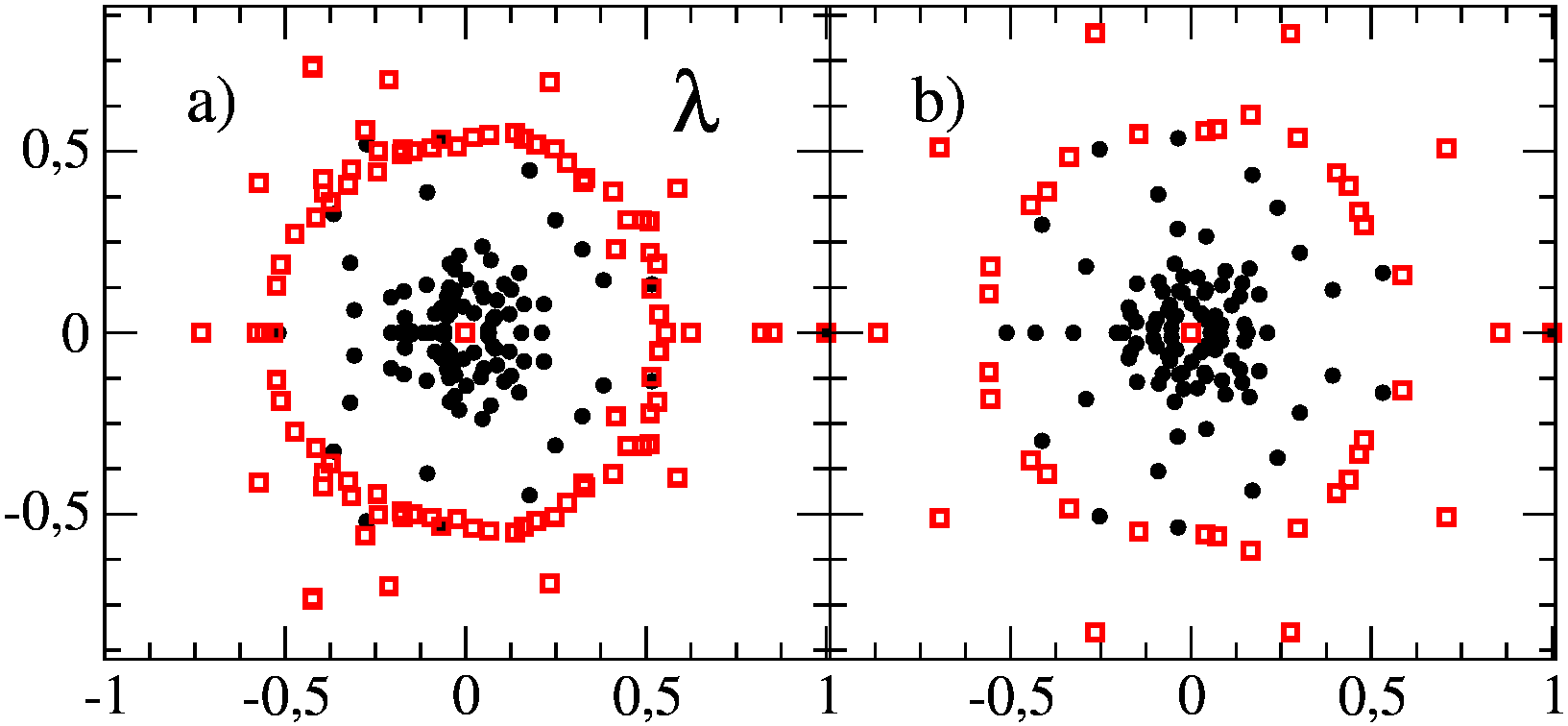
Figure 4: (color online) Largest eigenvalues of the quantum superoperator $e^{\Lambda}$ (with $\hbar_{\rm eff}=0.042$) and of the Perron-Frobenius superoperator (with $N=300$) for a) ($\gamma=0.33,k=6.86$), b) ($\gamma=0.33,k=6.8$). Black dots correspond to the quantum model while (red) gray squares to the classical one.

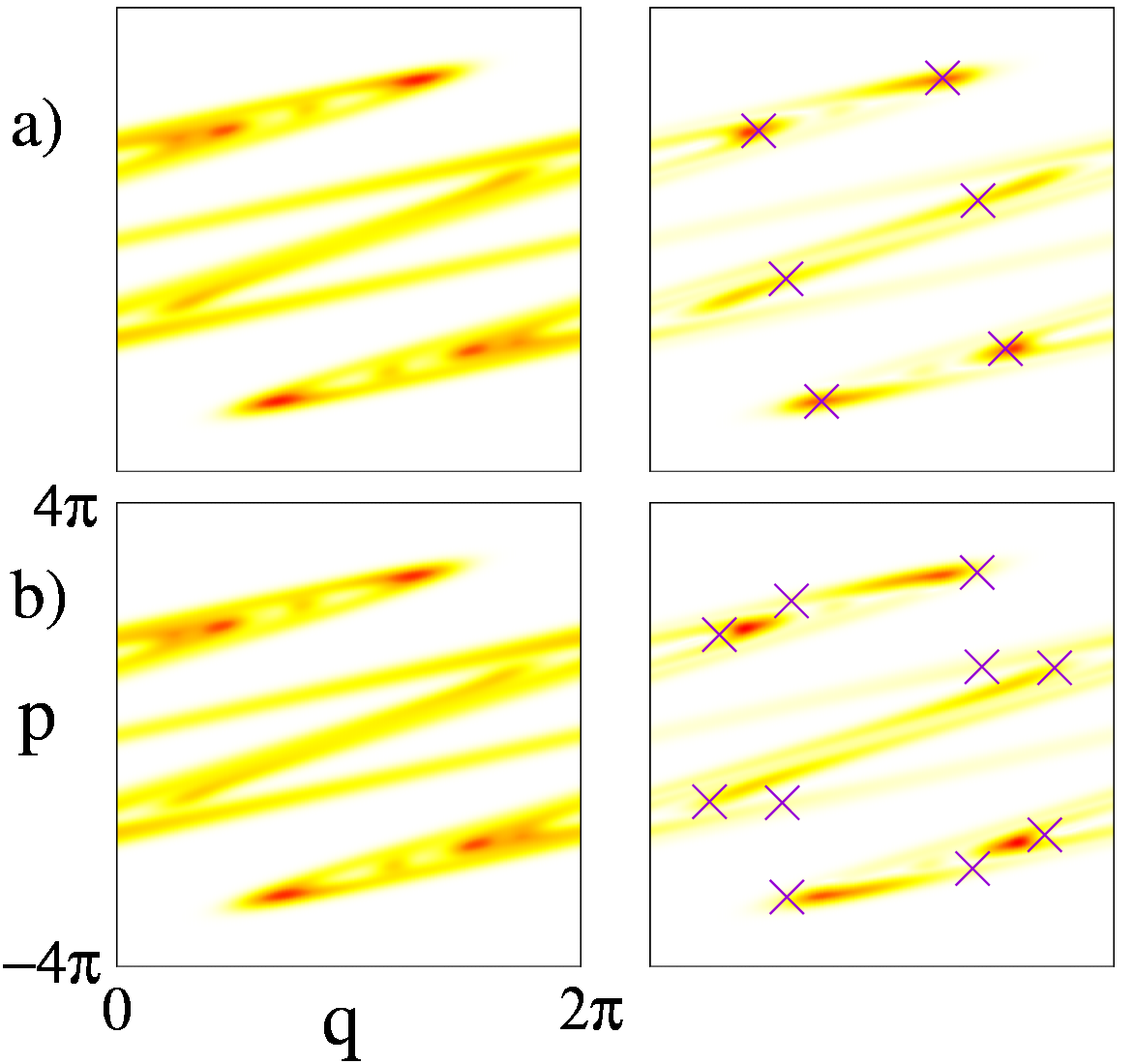
Figure 5: (color online) Husimi representation of the invariant state (left panel) and leading eigenstate (right panel) for a) ($\gamma=0.33,k=6.86$), b) ($\gamma=0.33,k=6.8$). $\hbar_{\rm eff}=0.042$. In the right panels the periodic points of the ISSs are marked with crosses.

IV Conclusions

The standard map is a paradigmatic model in the classical and the quantum chaos literature, while the dissipative version shares the same status for the theory of dissipative systems. Its classical parameter space shows a rich structure, proper of nonintegrable dissipative systems, which consists of a large regular region and a chaotic domain in which ISSs are embedded. As it has been established in previous works, these small stable structures are washed away by quantum fluctuations, implying that the equilibrium states (in regions other the regular region) have the structure of chaotic attractors, independently of their location in the chaotic sea.

In this work we have investigated how the presence of an ISS affects its neighborhood in parameter space by focusing on the spectral properties of the quantum mechanical superoperator. We have found that the ISSs play a fundamental role in the morphology of the leading eigenvectors of spectra obtained for parameters where they are present (at the classical level), but more interestingly, also at their vicinity. These eigenvectors turn out to be particularly long-lived and show a clear scarring by a limit cycle that belongs to the ISS. The second effect concerns the complex phases of the corresponding eigenvalues which are related to the periodicity of these limit cycles.

Our results strongly suggest that three factors are involved in the appearance of this mechanism (which shows another aspect of the parametrical tunneling). In the first place, the distance of the considered parameter space location to the ISS should be short in terms of the distance to other structures. Secondly, its size in parameter space should be greater or the same than other neighbouring regions. Finally, the period of the related periodic orbit should be short enough to be perceived by quantum mechanics (in fact, this is also an important property in order to even find them in the classical explorations Martins ). We conjecture that, given the paradigmatic nature of our model, these results can be considered to be generic properties of quantum dissipative systems.

References

- (1) U. Weiss, Quantum Dissipative Systems (World Scientific, Singapore, 2008).
- (2) M.A. Nielsen and I.L. Chuang, Quantum Computation and Quantum Information, Cambridge University Press (2000).
- (3) J. Preskill, Lecture Notes for Physics 229: Quantum Information and Computation, http://www.theory.caltech.edu/people/preskill/ph229/.
- (4) P. H. Jones, M. Goonasekera, D.R. Meacher, T. Jonckheere, and T.S. Monteiro, Phys. Rev. Lett. 98, 073002 (2007); T. Salger, S. Kling, T. Hecking, C. Geckeler, L. Morales-Molina, and M. Weitz, Science 326, 1241 (2009).
- (5) T. S. Monteiro, P. A. Dando, N. A. C. Hutchings, and M. R. Isherwood, Phys. Rev. Lett. 89, 194102 (2002); G. G. Carlo, G. Benenti, G. Casati, S. Wimberger, O. Morsch, R. Mannella, and E. Arimondo, Phys. Rev. A 74, 033617 (2006).
- (6) D. Vorberg, W. Wustmann, R. Ketzmerick, and A. Eckardt, Phys. Rev. Lett 111, 240405 (2013).
- (7) D. Kienzler, H.-Y. Lo, B. Keitch, L. de Clercq, F. Leupold, F. Lindenfelser, M. Marinelli, V. Negnevitsky, J. P. Home, Science 347, 53 (2015).
- (8) L. Bakemeier, A. Alvermann, and H. Fehske, Phys. Rev. Lett. 114, 013601 (2015).
- (9) M. Hartmann, D. Poletti, M. Ivanchenko, S. Denisov, and P. Hänggi, arXiv:1606.03896.
- (10) M. Ivanchenko, E. Kozinov, V. Volokitin, A. Liniov, I. Meyerov, S. Denisov, arXiv:1612.03444 (2016).
- (11) G. G. Carlo, A. M. F. Rivas, and M. E. Spina, Phys. Rev. E 84, 066201 (2011). M. E. Spina, A. M. F. Rivas, and G. G. Carlo, J. Phys. A: Math. Theor. 46, 475101 (2013).
- (12) L. Ermann and G.G. Carlo, Phys. Rev. E 91, 010903(R) (2015); G. G. Carlo, L. Ermann, A. M. F. Rivas, and M. E. Spina, Phys. Rev. E 93, 042133 (2016).
- (13) M.W. Beims, M. Schlesinger, C. Manchein, A. Celestino, A. Pernice, and W.T. Strunz Phys. Rev. E 91, 052908 (2015).
- (14) G.G. Carlo, Phys. Rev. Lett. 108, 210605 (2012).
- (15) E.G. Vergini and G.G. Carlo, J. Phys. A: Math. Gen. 33, 4717 (2000); H. Cao and J. Wiersig, Rev. Mod. Phys. 87, 61 (2015); L. Ermann, G.G. Carlo, and M. Saraceno, Phys. Rev. Lett. 103, 054102 (2009).
- (16) G. Schmidt and B.W.Wang, Phys. Rev. A 32, 2994 (1985).
- (17) G. Lindblad, Commun. Math. Phys. 48, 119 (1976).
- (18) T. Dittrich and R. Graham, Europhys. Lett., 7, 287 (1988).
- (19) R. Graham, Z. Phys. B Cond. Mat., 59, 75 (1985).
- (20) L. Ermann and D.L. Shepelyansky, Eur. Phys. J. B, 75, 299 (2010); K.M. Frahm, and D.L. Shepelyansky, Eur. Phys. J. B, 76, 57 (2010).
- (21) A collection of mathematical problems, S.M. Ulam, Interscience tracts in pure and applied mathematics 8, Interscience, New York, 1960.
- (22) G.W. Stewart, Matrix Algorithms Vol. II: Eigensystems (SIAM, Philadelphia, PA), 2001; L. Ermann, K.M. Frahm, and D.L. Shepelyansky, Rev. Mod Phys. 87, 1261 (2015).
- (23) L.C. Martins and J.A.C. Gallas, Int. J. Bifurc. Chaos 18, 1705 (2008).
- (24) W. Wenzel, O. Biham and C. Jayaprakash, Phys. Rev. A 43, 6550 (1991).