The Openpipeflow Navier–Stokes Solver

Abstract

Pipelines are used in a huge range of industrial processes involving fluids, and the ability to accurately predict properties of the flow through a pipe is of fundamental engineering importance. Armed with parallel MPI, Arnoldi and Newton–Krylov solvers, the Openpipeflow code can be used in a range of settings, from large-scale simulation of highly turbulent flow, to the detailed analysis of nonlinear invariant solutions (equilibria and periodic orbits) and their influence on the dynamics of the flow.
Website:  openpipeflow.org
Reference:  SoftwareX, 6, 124-127.
DOI:  10.1016/j.softx.2017.05.003

1 Motivation and significance

The flow of fluid through a straight pipe of circular cross-section is a canonical setting for the study of stability, transition and properties of turbulent flow. At low flow rates, the flow everywhere is in the direction parallel to the axis of the pipe, a simple ‘laminar’ flow. At larger flow rates it typically undergoes a transition to a complex ‘turbulent’ flow, characterised by an abundance of swirling eddies. As early as 1883, Reynolds observed that the transition from laminar to turbulent flow is highly dependent on perturbations of finite amplitude to the initial flow [1]. Nevertheless, he also noticed that the appearance of turbulence is consistent with respect to the value of the non-dimensional combination $D\,U/\nu$, at around 2000, where $U$ is the mean axial speed, $D$ the diameter of the pipe, and $\nu$ the kinematic viscosity. This combination is the now famous Reynolds Number, $Re=D\,U/\nu$, used in a huge range of systems involving fluids, where $D$ and $U$ are typical length and velocity scales for the system.

It has been known for some time that the Navier–Stokes equations together with the no-slip boundary conditions accurately predict the evolution of the flow pattern, e.g. the landmark prediction of supercritical transition to a roll pattern for the flow of water between rotating cylinders by G. I. Taylor [2] (transition due to linear instability beyond a critical rotation rate). Despite this development and the legacy of the work of Reynolds, the nature of subcritical transition (transition in the absence a linear instability) and the dynamics of pipe flow has largely remained a mystery. But much has changed following the discovery finite-amplitude solutions to the Navier–Stokes equations, for pipe flow as recently as 2003 [3]. These solutions, often referred to as ‘exact coherent states’ [4] are believed to embody the processes that sustain turbulence to and form a ‘skeleton’ for the dynamic paths taken by the evolving flow patterns. Comprehension of the nonlinear dynamics, particularly of transition in pipes, and likewise in Couette and channel flows, has progressed in leaps and bounds over the last decade, based on the study of these solutions. New more general families of solutions continue to be discovered, and their unstable manifolds are just beginning to be calculated [5, 6, 7, 8].

The code that has evolved into Openpipeflow has played a significant role in the realisation of this odyssey. Openpipeflow offers a more simplified approach than large computational fluid dynamics (CFD) packages – the aim during development has been to maintain a compact and readable code. Thus Openpipeflow is easily adapted for a given analysis and extendible to new numerical methods. The code has recently been upgraded with a substantially improved parallelisation, and continues to be augmented with new extensions, for example large-eddy simulation (LES).

Following the rapid expansion of computational resources that has occurred in recent times, pipe flow is a prime example of a ‘high-dimensional’ system that is receiving examination with methods previously limited to systems with only a few degrees of freedom, such as the Lorenz attractor or the Kuramoto–Sivashinsky equation; see e.g. [9, 10]. In the other direction, observations from large-scale simulations of pipe flow have inspired low-order models [11, 12]. Pipe flow also provides a simple setting for the development of computationally intensive new methods, such as adjoint optimisation techniques, e.g. [13].

2 Software description

Openpipeflow implements a second-order predictor-corrector scheme, with automatic time-step control, for simulation of flow on the cylindrical domain $(r,\theta,z)\,\in\,[0,1]\times[0,2\pi/m_{p})\times[0,2\pi/\alpha)$, where $m_{p}$ and $\alpha$ are parameters that determine spatial periodicity. Variables in the Navier–Stokes equations are discretised in the form

$$A(r,\theta,z)\,=\,\sum_{k<|K|}\,\sum_{m<|M|}A_{km}(r_{n})\,\mathrm{e}^{\mathrm{i}(\alpha kz+m_{p}m\theta)}\,,$$ (1)

$n=1..N$, where the points $r_{n}$ are distributed on $[0,1]$. By default the $r_{n}$ are located at the roots of a Chebyshev polynomial, bunched towards the boundaries to resolve large gradients that occur in the boundary layer. Derivatives in the radial dimension are calculated using finite differences, so that they may be evaluated using banded matrices. The number of points used, and hence the width of the bands, is an integer parameter; by default derivatives are calculated using 9 points, for which 1st/2nd order derivatives are calculated to 8th/7th order. Following the $3/2$ dealiasing rule, the sums are evaluated on $3K\times 3M$ grids in $z$ and $\theta$ respectively. Periodicity in $z$ is a commonplace approximation that has been shown to capture all the relevant physics of turbulent flow [14] and the transition to turbulent flow [9]. The dimension $\theta$ is naturally periodic ($m_{p}=1$). Rotational symmetry ($m_{p}=2,3,...$) is often applied, since finite-amplitude solutions typically satisfy rotational symmetry, or applied simply to reduce computational expense when the structures of interest are much smaller than the domain, e.g. near-wall vortices at large flow rates.

A pressure-Poisson equation (PPE) formulation is employed and an influence-matrix technique applied for the enforcement of boundary conditions [15]. Let $g$ be a vector of boundary conditions, written such that $\mbox{\boldmath$g$}=\mbox{\boldmath$0$}$ when they are satisfied. The influence-matrix technique has several nice features.:

• Alternative boundary conditions, e.g. slip or oscillations, are easily introduced by changing the single function that evaluates $g$;

• The usual no-slip and divergence conditions at the boundary are satisfied such that $\|\mbox{\boldmath$g$}\|$ is typically at the level of the machine epsilon for the given floating-point precision;

• Computational overhead is negligible compared to evaluation of non-linear terms;

• No stability issues have been observed.

Utilities and templates for runtime- and post-processing are included, including a Newton–Raphson solver for the calculation and continuation of invariant solutions. The Newton solver for the pipe flow, which has a multiple-shooting option (orbits may be split into multiple sections), calls a utility that implements a combined Krylov–Trust-region approach [16]. This Newton–Krylov–Trust-region utility is designed to be integrable with any simulation code.

Openpipeflow is written in Fortran90 and uses basic modules and derived types. Esoteric extensions to the programming language have been deliberately avoided. The code makes use of FFTW, LAPACK and NetCDF libraries. Optionally, for parallel use an MPI library is required.

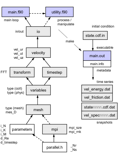
Figure 1: Code structure and program interaction. The MPI library is not required if $\texttt{\_Nr}=\texttt{\_Ns}=1$. To post-process data it is sufficient for a utility to inherit the io module. To process at run time, it is possible to inherit the whole main loop.

2.1 Software Architecture and Functionality

See Fig. 1 for a schematic of the code structure and program interaction. Once parameters are set and the code built, most jobs begin with a single initial condition, state.cdf.in. Outputs from another job, statennnn.cdf.dat, usually make the best initial conditions (nnnn is a 4-digit numeric label). A variety of possible initial conditions are provided in the database at openpipeflow.org. Truncation or interpolation of initial conditions with a different resolution is automatic.

A selection of utilities, plus templates for post-processing or runtime-processing, are described in the online manual.

2.2 Implementation details

Linear systems that originate from the implicit solution of the viscous terms in the Navier–Stokes equations are solved using banded matrices and LU-decomposition for each Fourier mode. Nonlinear terms are evaluated pseudospectrally.

Parallelisation is achieved via a split into _Nr radial and _Ns axial sections, and the work is divided over $\texttt{\_Np}=\texttt{\_Nr}\times\texttt{\_Ns}$ cores (#-defined symbols in parallel.h). Due to the form of the data transposes involved in the transforms between ‘collocated’ (Fourier) and physical space (type (coll) and type (phys)), the number of cores is limited to $N\times M$. This has been a distant limitation to date.

The recent upgrade to the two-dimensional split from the one-dimensional ‘wall-normal’ split (independent 2D-FFTs) not only extends the maximum number of cores from $N$ to $N\times M$, but also reduces the number of messages that must be sent. The transform involves two stages of FFTs and transposes, but each transpose involves only _Nr or _Ns cores. For a transpose involving $p$ cores, each core must send $p-1$ messages. Therefore, choosing $\texttt{\_Nr}\approx\texttt{\_Ns}~{}\approx\sqrt{\texttt{\_Np}}$, the number of messages is $O(2\sqrt{\texttt{\_Np}})$ versus $O(\texttt{\_Np})$. This can substantially reduce time lost in latency due to the time setting up communications. Further details can be found on the Core Implementation page of the online manual.

3 Illustrative Examples

3.1 Modelling a Coriolis force

Does the Coriolis force, an extra force term due to rotation of Earth, affect the flow in experiments? The file utils/Coriolis.f90 is an example utility is provided with the distribution that models this case.

The main loop of the core code already includes several calls to a null function at key points during the timestepping process; see var_null(flag) in program/main.f90. The flag may be used to detect the stage at which the function has been called. Here, we replace the null function with the function in Coriolis.f90 and detect the case flag==2, which indicates that nonlinear terms have just been evaluated. At this point we add the Coriolis forces to the nonlinear terms. Note that no changes to the core files, including main.f90, are necessary.

Figure 2 shows the mean axial flow profile for laminar and turbulent flow at an Ekman number $E=\nu/(2\Omega D^{2})=1$ for a pipe with axis oriented east-west, perpendicular to the rotation of axis for any latitude. For a pipe filled with water at 20$\,{}^{\circ}$C, this corresponds to a diameter $D$ of approximately 8.3cm; $Re=5300$ in all cases, U_cl is the centreline speed for laminar flow at the same mean flow rate, and $\mathrm{R}=D/2$ is the pipe radius. For this $Re$, laminar flow shows a substantial response, and the profile is similar to those reported in [17]. Turbulent flow, however, shows no asymmetry. The turbulent mean profile is indiscernible from the documented test case [14].

Figure 2: Response of flow at $Re=5300$ to a Coriolis force. Solid: Laminar flow, $E\to\infty$ (no rotation). Short-dash: Laminar flow, $E=1$. Long-dash: Turbulent flow, $E=1$.

3.2 Unstable manifold of a travelling wave solution

A travelling wave solution is an equilibrium when considered in a frame moving at its phase speed. In this case we consider the ‘upper branch’ solution known as N2_ML, Fig. 3, which in its symmetry subclass has a single unstable complex eigenvalue, $0.00620+0.0183\,\mathrm{i}\,(\mathrm{U}_{\mathrm{cl}}/\mathrm{R})$ (after one rotation it expands by a factor $8.4$); $Re=2400$, $\alpha=1.25$, $m_{p}=2$; see [18] for further details. For a given nearby state, the Newton–Krylov utility (newton.f90) can find such solutions and output their leading unstable eigenvectors (solution state1000.cdf.dat and real and imaginary parts of the leading eigenvector, state1001.cdf.dat, state1002.cdf.dat; available at the online Database). To visualise the unstable manifold, we use a utility (addstates.f90) to add small multiples ($\approx 10^{-4}\times$) of the real part of the eigenvector to the solution, then use these as initial conditions (state.cdf.in) for a set of simulations. Figure 4 shows a projection of the unstable manifold of N2_ML, as an outward spiral, with deformation at larger amplitudes due to nonlinearity. The coordinates are the kinetic energy $E$, energy input from the applied pressure gradient $I$, and energy dissipation $D$, each normalised by their respective value for laminar flow (columns of output vel_totEID.dat).

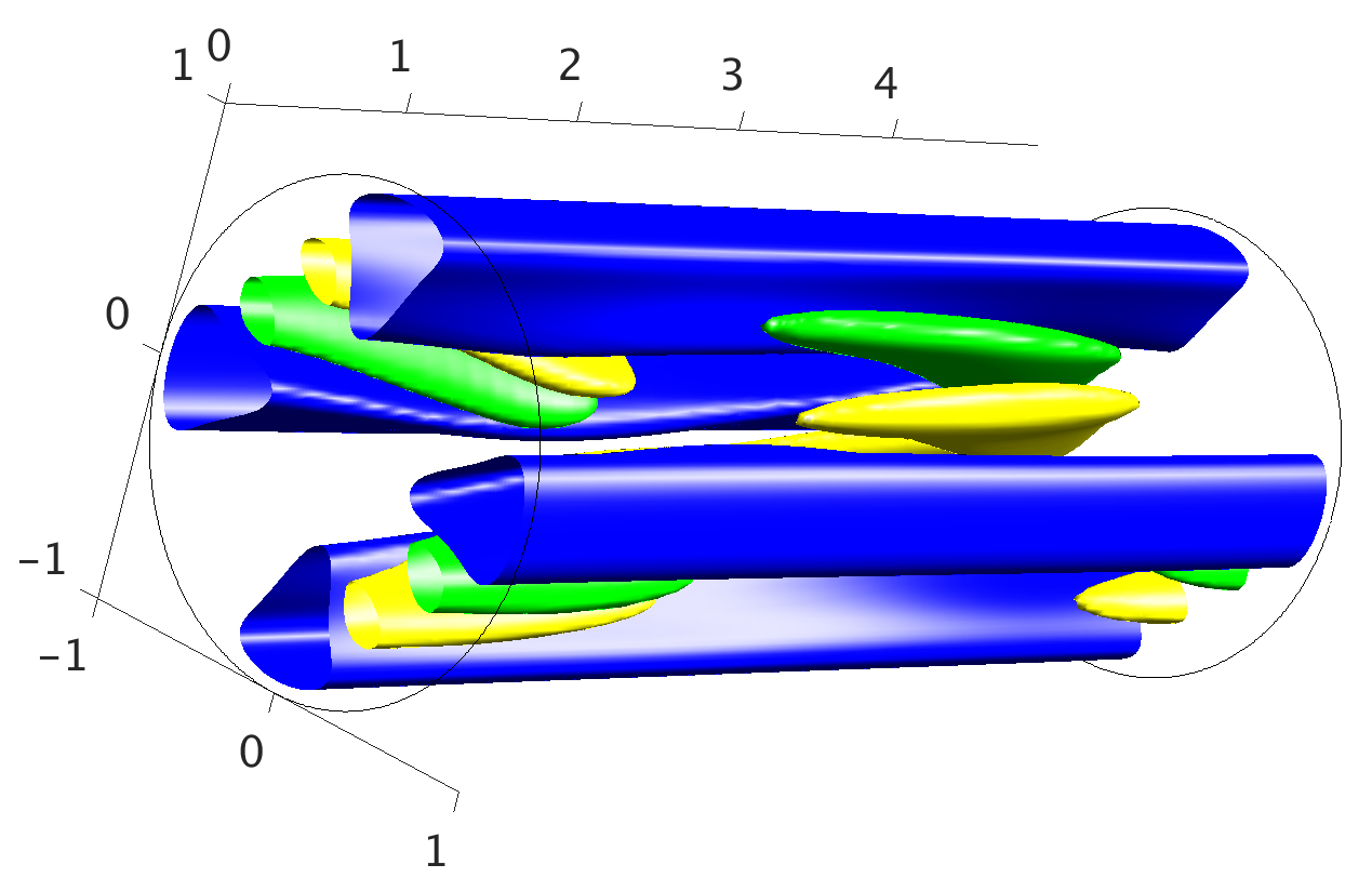
Figure 3: N2_ML solution. (blue) Slow ‘streaks’ – axial flow slower than the mean flow profile by $>0.07$. (yellow and green) ‘vortices’ – axial vorticity $>0.2$ and $<-0.2$.

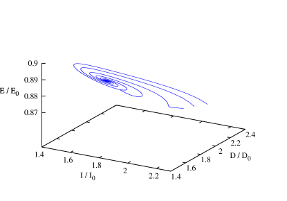
Figure 4: Projection of the unstable manifold of the N2_ML travelling wave solution.

4 Impact and conclusions

The Openpipeflow solver aims to provide a fast but flexible code, that can be use for state-of-the art research in the study of turbulent flows and transition.

Pipe flow is a classical setting for the development of methods for modelling and analysing dynamical systems, and Openpipeflow has been used by several groups around the world to make an important contribution to developments in our understanding of subcritical transition, e.g. [7, 8, 11, 12, 5, 19].

From these developments have arisen many new opportunities. From the theoretical viewpoint, open issues relate to comprehension of the role of newly discovered equilibria and periodic orbits. Such states are believed to provide a skeleton for the dynamics, but describing the topology of the state space for turbulence remains a challenging and active area. Pipe flow, and the study of shear flows in general, draw interest from a range of branches of mathematics and theoretical physics, e.g. pattern formation, control theory, statistical physics, experimental physics. It is an active area of cross-fertilisation for the development of mathematical and numerical methods.

From a more practical viewpoint, the dynamical systems approach is being applied in the modelling of other important flows, e.g. flows of fluids of complex rheology, e.g. stress-dependent viscosity, particulate flows and multiphase flows. The study of ‘high Reynolds number’ flows is also being influenced via application of dynamical systems techniques using LES.

Openpipeflow stands well placed to make an increasingly valuable contribution to this effort. Alongside the application of methods drawn from chaos theory, extensions to Openpipeflow have just been added for shear-thinning fluids and LES, for example. From a research perspective, plenty of exciting new developments are in the pipeline.

References

- [1] O. Reynolds, An experimental investigation of the circumstances which determine whether the motion of water shall be direct or sinuous, and the law of resistance in parallel channels, Proc. Roy. Soc. Lond. Ser A 174 (1883) 935–982.
- [2] G. I. Taylor, Stability of a viscous liquid contained between two rotating cylinders, Phil. Trans. Royal Soc. A 223 (1923) 289–343.
- [3] H. Faisst, B. Eckhardt, Traveling waves in pipe flow, Phys. Rev. Lett. 91 (2003) 224502.
- [4] F. Waleffe, Exact coherent structures in channel flow, J. Fluid Mech. 435 (2001) 93–102.
- [5] C. C. T. Pringle, Y. Duguet, R. R. Kerswell, Highly symmetric travelling waves in pipe flow, Phil. Trans. Royal Soc. A 367 (2009) 457–472.
- [6] A. de Lozar, F. Mellibovsky, M. Avila, B. Hof, Edge state in pipe flow experiments, Phys. Rev. Lett. 108 (2012) 214502. doi:10.1103/PhysRevLett.108.214502.
- [7] M. Avila, F. Mellibovsky, N. Roland, B. Hof, Streamwise-localized solutions at the onset of turbulence in pipe flow, Phys. Rev. Lett. 110 (2013) 224502. doi:10.1103/PhysRevLett.110.224502.
- [8] M. Chantry, A. P. Willis, R. R. Kerswell, Genesis of streamwise-localized solutions from globally periodic traveling waves in pipe flow, Phys. Rev. Lett. 112 (2014) 164501. doi:10.1103/PhysRevLett.112.164501.
- [9] K. Avila, D. Moxey, A. de Lozar, M. Avila, D. Barkley, B. Hof, The onset of turbulence in pipe flow, Science 333 (2011) 192–196. doi:10.1126/science.1203223.
- [10] A. P. Willis, K. Y. Short, P. Cvitanović, Symmetry reduction in high dimensions, illustrated in a turbulent pipe, Phys. Rev. E 93 (2016) 022204. doi:10.1103/PhysRevE.93.022204.
- [11] D. Barkley, B. Song, V. Mukund, G. Lemoult, M. Avila, B. Hof, The rise of fully turbulent flow, Nature 526 (7574) (2015) 550–553.
- [12] H.-Y. Shih, T.-L. Hsieh, N. Goldenfeld, Ecological collapse and the emergence of travelling waves at the onset of shear turbulence, Nature Physics 12 (2015) 245–248.
- [13] C. C. Pringle, A. P. Willis, R. R. Kerswell, Minimal seeds for shear flow turbulence: using nonlinear transient growth to touch the edge of chaos, Journal of Fluid Mechanics 702 (2012) 415–443.
- [14] J. G. M. Eggels, F. Unger, M. H. Weiss, J. Westerweel, R. J. Adrian, R. Freidrich, F. T. M. Nieuwstadt, Fully developed turbulent pipe flow: a comparison between direct numerical simulation and experiment, J. Fluid Mech. 268 (1994) 175–209.
- [15] A. Guseva, A. P. Willis, R. Hollerbach, M. Avila, Transition to magnetorotational turbulence in Taylor–Couette flow with imposed azimuthal magnetic field, New Journal of Physics 17 (9) (2015) 093018.
- [16] D. Viswanath, Recurrent motions within plane Couette turbulence, J. Fluid Mech. 580 (2007) 339–358. doi:10.1017/S0022112007005459.
- [17] A. Draad, F. Nieuwstadt, The earth’s rotation and laminar pipe flow, Journal of Fluid Mechanics 361 (1998) 297–308.
- [18] A. P. Willis, P. Cvitanović, M. Avila, Revealing the state space of turbulent pipe flow by symmetry reduction, J. Fluid Mech. 721 (2013) 514–540. doi:10.1017/jfm.2013.75.
- [19] A. P. Willis, R. R. Kerswell, Coherent structures in localised and global pipe turbulence, Phys. Rev. Lett. 100 (2008) 124501.