Quasi-Reliable Estimates of Effective Sample Size

Abstract

The efficiency of a Markov chain Monte Carlo algorithm might be measured by the cost of generating one independent sample, or equivalently, the total cost divided by the effective sample size, defined in terms of the integrated autocorrelation time. To ensure the reliability of such an estimate, it is suggested that there be an adequate sampling of state space—to the extent that this can be determined from the available samples. A possible method for doing this is derived and evaluated.

1 Introduction

Markov chain Monte Carlo (MCMC) methods are very widely used to estimate expectations of random variables, since they are often the only methods applicable to complicated and high dimensional distributions. Their accuracy is low relative to computational effort, so it is particularly important to have reliable error estimates. Due to the correlated nature of MCMC samples, a variance estimate for $N$ samples uses the effective sample size $\mathit{ESS}$ rather than $N$ in the denominator. The effective sample size for a random variable can be computed from its integrated autocorrelation time. Proposed in this paper is a more reliable estimate of $\mathit{ESS}$, particularly for multimodal distributions.

This study is motivated by an interest in designing more efficient MCMC samplers. For evaluating performance of MCMC methods, there is wide support among both statisticians, e.g., Charles Geyer (1992, page 11) [4], and physicists, e.g., Alan Sokal (1997, page 13) [15] for using as a metric the cost of an independent sample:

$$\frac{N}{\mathit{ESS}}\times\mbox{cost per step}=\tau\times\mbox{cost per step},$$

where $\tau$ is the integrated autocorrelation time.

Similarly, for evaluating accuracy of MCMC estimates, it is deemed essential, e.g., Alan Sokal (page 11) [15] again, to know the autocorrelation time. Nonetheless, MCMC is often used for problems for which $\mathit{ESS}$ is very small, perhaps even less than 1. How should such problems be handled? One option is to avoid claims of sampling and instead designate the simulation as “exploration”. Another option is to change the problem: For example, use a simpler model. A coarsened model with error bars is better than a refined model without error bars (because then the limitations are more explicit). Alternatively, artificially limit the extent of state space, and adjust conclusions accordingly.

A computed estimate of the integrated autocorrelation time might be marred by incomplete sampling—at least in the case of multimodal distributions. Without additional information, there is no foolproof way of detecting convergence, so reliability is impractical in general. So the goal is instead quasi-reliability, which is defined to mean apparent good coverage of state space—ensuring thorough sampling of that part of state space that has already been explored, to minimize the risk of missing an opening to an unexplored part of state space. More concretely, it might mean thorough sampling of those modes that have already been visited, to minimize the risk of missing an opening to yet another mode.

This article makes a couple of contributions towards more reliable estimates of effective sample size:

1. A quantity is derived for measuring thoroughness of sampling that is simple to describe and relatively easy to estimate, namely, the longest autocorrelation time over all possible functions defined on state space, denoted by $\tau_{\max}$. This quantity has two advantages over estimates of $\tau$ only for functions of interest. (i) It is more likely to indicate the existence of a transition path to a mode that has not been visited. (ii) It is more reliably estimated with finite sampling than is $\tau$ for just any function: even though a function of interest might have a small value of $\tau$, a reliable estimate of its autocorrelation function and integrated autocorrelation time $\tau$ may well require a number of samples dictated by $\tau_{\max}$.

2. An algorithm is constructed for estimating $\tau_{\max}$, assuming the availability of a method for estimating the integrated autocorrelation time $\tau$ for an arbitrary function, and evidence is presented for the utility of this algorithm.

Section 2 of this article establishes notation by reviewing needed concepts and methods. It presents the definition and role of the integrated autocorrelation $\tau$. It defines a forward transfer operator that comprises transition probabilites of the MCMC process. And it presents the notion of a lag window for estimating $\tau$ for a finite number of samples $N$.

Section 3 is the heart of this article. It begins with an example illustrating how it is possible to have an apparently reliable esimate of $\tau$ that is far too small. It then defines thorough sampling to mean that (with, say, 95% confidence) the fraction of samples from any given subset of state space should differ from the actual probability by no more than some specified tolerance $\mathit{tol}$. It is shown that this is achieved if $N\geq\tau_{\max}/\mathit{tol}^{2}$. An approximate maximum is obtained by considering arbitrary linear combinations of a finite set of basis functions. This results in a generalized eigenvalue problem. The matrices are shown to be symmetric not only for reversible MCMC methods but also for a class of “modified” reversible MCMC methods that includes generalized hybrid Monte Carlo samplers and reversible (inertial) Langevin integrators.

Section 4 tests the methodology on 4 examples. A 1-dimensional Gaussian distribution is used to confirm the correctness of the theory. A sum of 2 Gaussians is used as a simple example of a multimodal problem, which demonstrates the advantage of seeking the longest autocorrelation time. A 2-layer single-node neural network is used to capture the flavor of machine learning applications. It yields a large enough estimate of $\tau_{\max}$ to serve as a warning that an apparently large sample size is inadequate, unlike the $\tau$ estimate for the quantity of interest. Finally a logistic regression example confirms again the wisdom of seeking the longest autocorrelation time $\tau_{\max}$.

Section 5 is a brief discussion and conclusion.

Initial attempts to estimate the integrated autocorrelation time employed a small computer program called acor [5]. Due to concerns about its reliability, Appendix A derives an alternative method for defining the lag window under a couple of simplyfying assumptions, one of which becomes more credible for observables having a large value of $\tau$. Experiments indicate slightly more reliable estimates compared to acor.

2 Preliminaries and Background

Given a probability density $\rho_{\mathrm{q}}(\mathbf{q})$, $\mathbf{q}\in\mathbb{R}^{d}$, known only up to a multiplicative factor, the aim is to compute observables $\mathbb{E}[u(\mathbf{Q})]$, which are expectations for specified functions $u(\mathbf{q})$. Note here the use of upper case for random variables.

Consider a Markov chain $\mathbf{Q}_{0}\rightarrow\mathbf{Q}_{1}\rightarrow\cdots\rightarrow\mathbf{Q}_{N-1}$ that is ergodic with stationary density $\rho_{\mathrm{q}}(\mathbf{q})$. Also, assume $\mathbf{Q}_{0}\sim\rho_{\mathrm{q}}(\mathbf{q})$. To estimate an observable, use

$$\mathbb{E}[u(\mathbf{Q})]\approx\overline{U}=\frac{1}{N}\sum_{n=0}^{N-1}u(\mathbf{Q}_{n}),$$

but use just one realization $\mathbf{q}_{0}\rightarrow\mathbf{q}_{1}\rightarrow\cdots\rightarrow\mathbf{q}_{N-1}$, assuming samples are renumbered to omit those prior to equilibration/burnin.

2.1 Variance of the estimated mean

There are a variety of methods for estimating the variance of the estimated mean. Most appealing [4] are those that expoit the fact that the sample is generated by a Markov chain. The variance of the estimated mean is given by

$$\mathrm{Var}[\overline{U}]=\frac{1}{N}\mathrm{Var}[u(\mathbf{Q})]\left(1+2\sum_{k=1}^{N-1}\left(1-\frac{k}{N}\right)\frac{C(k)}{C(0)}\right)$$

where the autocovariances

$$C(k)=\mathbb{E}[(u(\mathbf{Q}_{0})-\mu)(u(\mathbf{Q}_{k})-\mu)],$$

with $\mu=\mathbb{E}[u(\mathbf{Q})]$. In the limit $N\rightarrow\infty$,

$$\mathrm{Var}[\overline{U}]=\frac{1}{N}\mathrm{Var}[u(\mathbf{Q})]\tau+o(\frac{1}{N})$$

where $\tau$ is the integrated autocorrelation time.

$$\tau=1+2\sum_{k=1}^{+\infty}\frac{C(k)}{C(0)}.$$ (1)

An estimate of covariances is provided by Ref. [11, pp. 323–324]:

$$C_{N}(k)=\frac{1}{N}\sum_{n=0}^{N-k-1}(u(\mathbf{q}_{n})-\overline{u})(u(\mathbf{q}_{n+k})-\overline{u}).$$

2.2 Forward transfer operator

Some MCMC samplers augment state variables $\mathbf{q}$ with auxiliary variables $\mathbf{p}$, e.g., momenta, extend the p.d.f. to $\rho(\mathbf{q},\mathbf{p})$ so that

$$\int\rho(\mathbf{q},\mathbf{p})\mathrm{d}\mathbf{p}=\rho_{\mathrm{q}}(\mathbf{q}),$$

and make moves in extended state space $\mathbf{z}_{0}\rightarrow\mathbf{z}_{1}\rightarrow\cdots\rightarrow\mathbf{z}_{N-1}$ where $\mathbf{z}=(\mathbf{q},\mathbf{p})$.

Associated with the MCMC propagator is an operator $\mathcal{F}$, which maps a relative density $u_{n-1}=\rho_{n-1}/\rho$ for $\mathbf{Z}_{n-1}$ to a relative density $u_{n}=\rho_{n}/\rho$ for $\mathbf{Z}_{n}$:

$$u_{n}=\mathcal{F}u_{n-1}$$

where

$$\mathcal{F}u_{n-1}(\mathbf{z})=\frac{1}{\rho(\mathbf{z})}\int\rho(\mathbf{z}|\mathbf{z}^{\prime})u_{n-1}(\mathbf{z}^{\prime})\rho(\mathbf{z}^{\prime})\mathrm{d}\mathbf{z}^{\prime}$$

and $\rho(\mathbf{z}|\mathbf{z}^{\prime})$ is the transition probability density for the chain [14]. Note that $u\equiv 1$ is an eigenfunction of $\mathcal{F}$ for eigenvalue $\lambda_{1}=1$.

The error in the probability density, starting from $\rho_{0}(\mathbf{q})=\delta(\mathbf{q}-\mathbf{q}_{0})$, is

$$\frac{1}{N}\sum_{n=0}^{N-1}\rho_{n}-\rho=\rho\frac{1}{N}(1-\mathcal{F}_{0})^{-1}(1-\mathcal{F}_{0}^{N})\frac{\rho_{0}-\rho}{\rho}$$

where $\mathcal{F}_{0}$ is $\mathcal{F}$ with the eigenvalue 1 removed, i.e., $\mathcal{F}_{0}u=\mathcal{F}u-\mathbb{E}[u(\mathbf{Q})]$. From this, one sees that the error is proportional to the reciprocal of the spectral gap $|1-\lambda_{2}|$, where $\lambda_{2}$ is the nonunit eigenvalue of $\mathcal{F}$ nearest 1. This, however, is not the relevant quantity—in general (see 3.1).

2.3 Error in estimates of integrated autocorrelation time

The standard deviation of the statistical error in the estimate of $\tau$ from Eq. (1) grows with the number of terms taken; more specifically, it is approximately $\sqrt{M/N}\tau$ where $M$ is the number of terms [15, Eqs. (3.19)]. Therefore, one uses instead

$$\tau\approx 1+2\sum_{k=1}^{N-1}w(k)\frac{C_{N}(k)}{C_{N}(0)}$$

where $w(k)$ is a decreasing weight function known as a lag window.

The tiny program acor uses a lag window that is $1$ for $k$ from $0$ to $M-1$ and $0$ for the rest where $M$ is the smallest number that exceeds the estimated $\tau$ by a factor of 10. It requires the number of samples $N$ to exceed $100\tau$.

3 Thorough Sampling

Depending on estimates of the ESS for just the observables of interest can be deceptive.

Consider a mixture of 2 Gaussians,

$$-\log\rho(q_{1},q_{2})= \frac{1}{2}(36(q_{1}+1)^{2}+(q_{2}-3)^{2})$$ (2)

$$+\frac{1}{2}((q_{1}-2)^{2}+36q_{2}^{2})+\mbox{const},$$

whose combined basin has an L shape with a barrier at the corner of the L. For a sampler, consider the use of Euler-Maruyama Brownian dynamics (w/o rejections), defined in Sec. 3.3. A realization of a sampling trajectory is given in Figure 1. For the realization shown there, the trajectory makes the first transition around $N=1000$.

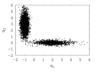
(a) 5000 samples

(b) Trajectories of $q_{1}$ and $q_{2}$

Figure 1: Example trajectory for the L-shaped mixture of Gaussians distribution.

Figure 2 shows the estimated integrated autocorrelation time and the effective sample size as a function of the sample size. To consider the question of thorough sampling, suppose that $\mathit{ESS}=100$ is regarded adequate for estimating observables. Just before the $q_{1}$ curve jumps, the ESS is much greater than 100 indicating thorough sampling. This is misleading since after the jump the ESS drops dramatically. On the other hand, the $q_{2}$ curve more reliably detects thorough sampling. Note that if the trajectory starts from the vertical leg of the ”L”, the behavior of $q_{1}$ and $q_{2}$ are swapped. This implies that a general observable that is independent of the starting point and can capture the “hardest” move is needed for better detecting convergence.

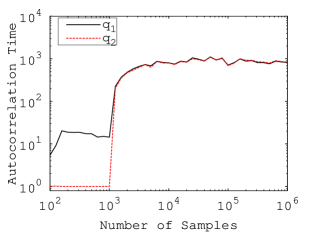
(a) Autocorrelation time

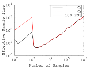
(b) Effective sample size

Figure 2: The autocorrelation time and the effective sample size vs. the number of samples in the L-shaped mixture of Gaussians problem.

3.1 Definition of thorough sampling

Good coverage of state space might be defined as follows: for any subset $A$ of (unextended) state space, an estimate $\overline{1_{A}}$ of $\mathbb{E}[1_{A}(\mathbf{Q})]=\Pr(\mathbf{Q}\in A)$ satisfies

$$\mathrm{Var}[\overline{1_{A}}]\leq\frac{1}{4}\mathit{tol}^{2}.$$

This would ensure 95% confidence that the proportion of samples for any subset $A$ is not off by more than $\mathit{tol}$. Since

$$\mathrm{Var}[\overline{1_{A}}]\approx\tau_{A}\frac{1}{N}\mathrm{Var}[1_{A}(\mathbf{Q})]\leq\frac{1}{4N}\tau_{A},$$

it is enough to have

$$\frac{1}{4N}\tau_{A}\leq\frac{1}{4}\mathit{tol}^{2}\quad\mbox{for all }A.$$ (3)

There may be permutations $P$ such that $\rho_{\mathrm{q}}(P\mathbf{q})=\rho_{\mathrm{q}}(\mathbf{q})$ and $u(P\mathbf{q})=u(\mathbf{q})$ for all interesting $u$. Then, it is appropriate to weaken the definition of good coverage by including only those $A$ for which $1_{A}(P\mathbf{q})=1_{A}(\mathbf{q})$.

To facilitate analysis, introduce the inner product

$$\langle v,u\rangle=\int\overline{v(\mathbf{z})}u(\mathbf{z})\rho(\mathbf{z})\,\mathrm{d}\mathbf{z}.$$

Note that $\langle 1,u\rangle$ is the expectation $\mathbb{E}[u(\mathbf{Z})]$ of $u(\mathbf{Z})$. One can show by induction that the cross covariance

$$\mathbb{E}[v(\mathbf{Z}_{0})u(\mathbf{Z}_{k})]=\langle\mathcal{F}^{k}v,u\rangle.$$

and, in particular, $C(k)=\langle\mathcal{F}^{k}u,u\rangle$.

For simplicity, instead of just indicator functions $1_{A}(\mathbf{q})$, consider arbitrary functions in

$$W= \{u=u(\mathbf{q})~{}|~{}\mathbb{E}[u(\mathbf{Q})]=0,$$

$$u(P\mathbf{q})=u(\mathbf{q})\mbox{ for symmetries }P\},$$

and define thorough sampling using

$$\tau_{\max}=\max_{u\in W}\left(1+2\sum_{k=1}^{+\infty}\frac{C(k)}{C(0)}\right)$$

in Eq. (3). The maximum autocorrelation time can be rewritten as

$$\tau_{\max}= \max_{u\in W}\left(1+2\sum_{k=1}^{+\infty}\frac{\langle\mathcal{F}^{k}u,u\rangle}{\langle u,u\rangle}\right)$$

$$= \max_{u\in W}\frac{\langle g(\mathcal{F})u,u\rangle}{\langle u,u\rangle}$$

where

$$g(\lambda)=1+2\lambda/(1-\lambda).$$

For reversible samplers, the spectral gap is intimately related to $\tau_{\max}$. If $\tau_{\max}$ were the maximum over all $u(\mathbf{z})$, then

$$\tau_{\max}=\frac{1+\lambda_{2}}{1-\lambda_{2}}.$$

where $\lambda_{2}$ is the second largest eigenvalue of the transfer operator.

3.2 Spatial discretization

For computational purposes, the idea is to seek a function that comes close to maximizing the autocorrelation time by considering a linear combination $u(\mathbf{q})=\mathbf{a}^{\mathsf{T}}\mathbf{u}(\mathbf{q})$ of given basis functions $u_{i}\in W$ where the $a_{i}$ are to be determined. (In practice, only the estimated mean of the function $u(\mathbf{q})$ vanishes.) Then its autocovariance

$$C(k)=\langle\mathcal{F}^{k}u,u\rangle=\mathbf{a}^{\mathsf{T}}C_{k}\mathbf{a}$$

where

$$C_{k}=\langle\mathcal{F}^{k}\mathbf{u},\mathbf{u}^{\mathsf{T}}\rangle=\mathbb{E}[\mathbf{u}(\mathbf{Q}_{0})\mathbf{u}(\mathbf{Q}_{k})^{\mathsf{T}}]$$

and

$$\tau_{\max}\approx\max_{\mathbf{a}}\frac{\mathbf{a}^{\mathsf{T}}K\mathbf{a}}{\mathbf{a}^{\mathsf{T}}C_{0}\mathbf{a}}\quad\mbox{where }K=C_{0}+2\sum_{k=1}^{+\infty}C_{k}$$

—a generalized eigenvalue problem (arising from maximizing a Rayleigh quotient).

Linear functions $u_{i}(\mathbf{q})=q_{i}$ are suggested as a general choice.

3.3 Symmetry of cross covariance matrices

The matrix $C_{0}$ is symmetric positive definite, if the components of $\mathbf{u}$ are linearly independent. The eigenvalue problem is well conditioned if $K$ is a symmetric matrix. Symmetry of $K$ does not hold for every sampler. Even when $K$ is symmetric, its finitely sampled estimate is not, so using the symmetric part can reduce sampling error.

A reversible MCMC samplers is defined to be one that satisfies detailed balance:

$$\rho(\mathbf{z}^{\prime}|\mathbf{z})\,\rho(\mathbf{z})=\rho(\mathbf{z}|\mathbf{z}^{\prime})\,\rho(\mathbf{z}^{\prime})$$

Examples of reversible samplers include

1. a Brownian sampler, the Euler-Maruyama discretization of Brownian dynamics coupled with a Metropolis-Rosenbluth-Rosenbluth-Teller-Teller  [10] acceptance test (known as MALA in the statistics literature [13]),

2. hybrid Monte Carlo  [2],

3. generalized hybrid Monte Carlo [6], with each step followed by a momentum flip,

4. a reversible Langevin integrator, with every fixed number of steps followed by a momentum flip (see below). Note that reversible has a different meaning for integrators than it does for samplers.

These last two samplers augment state space with momentum variables.

The momentum flip of the last two enumerated samplers defeats the purpose of augmenting state space with momenta. Indeed, reversing the momentum flip leads to more rapid mixing. More generally, a modified reversible propagator effectively couples the reversible substep $\mathbf{z}_{n-1}\rightarrow\bar{\mathbf{z}}_{n}$ with a substep,

$$\mathbf{z}_{n}=R(\bar{\mathbf{z}}_{n}),$$

where $R$ satisfies $R\circ R=\mathrm{id}$ and $\rho\circ R=\rho$. For a momentum flip, $R(\mathbf{q},\mathbf{p})=(\mathbf{q},-\mathbf{p})$.

Following is an example of a reversible Langevin integrator. Let $F(\mathbf{q})=-\nabla_{\mathbf{q}}\log\rho(\mathbf{q},\mathbf{p})$. Then each step of the integrator consists of the following five stages:

• $\mathbf{p}:=\mathbf{p}+\frac{1}{2}\Delta tF(\mathbf{q})$

• $\mathbf{q}:=\mathbf{q}+\frac{1}{2}\Delta t\mathbf{p}$

• $\mathbf{p}:=\sqrt{1-2\gamma\Delta t}\mathbf{p}+\sqrt{2\gamma\Delta t}\mathcal{N}(0,I)$

• $\mathbf{q}:=\mathbf{q}+\frac{1}{2}\Delta t\mathbf{p}$

• $\mathbf{p}:=\mathbf{p}+\frac{1}{2}\Delta tF(\mathbf{q})$

The dynamics of this integrator has a precise stationary density. It differs from the desired density [8] by $\mathcal{O}(\Delta t^{2})$. Such error is much smaller than statistical error. The Euler-Leimkuhler-Matthews integrator [7] is the special case $\gamma=1/(2\Delta t)$ of this, and it has the remarkable property of retaining second order accuracy. Since applying a momentum flip has no effect in this case, it is a reversible MCMC propagator. (The Euler-Leimkuhler-Matthews integrator can be expressed as a Markov chain in $\mathbf{q}$-space if post-processing is employed [16].)

For a modified reversible propagator, the forward transfer operator is a product

$$\mathcal{F}=\mathcal{R}\bar{\mathcal{F}},$$

where $\bar{\mathcal{F}}$ is the forward transfer operator of the reversible substep and $\mathcal{R}$ is the operator for the added substep $\mathbf{z}_{n}=R(\bar{\mathbf{z}}_{n})$:

$$u_{n}=\mathcal{R}\bar{u}_{n-1}$$

where

$$\mathcal{R}\bar{u}_{n-1}(\mathbf{z})=\frac{1}{\rho(\mathbf{z})}\int\delta(\mathbf{z}-R(\mathbf{z}^{\prime}))\bar{u}_{n-1}(\mathbf{z}^{\prime})\rho(\mathbf{z}^{\prime})\mathrm{d}\mathbf{z}^{\prime}.$$

It can be shown that the operators $\bar{\mathcal{F}}$ and $\mathcal{R}$ are self adjoint:

$$\langle\bar{\mathcal{F}}g,f\rangle=\langle g,\bar{\mathcal{F}}f\rangle\quad\mbox{and}\quad\langle\mathcal{R}g,f\rangle=\langle g,\mathcal{R}f\rangle.$$

Additionally, assume $\mathcal{R}\mathbf{u}(\mathbf{q})=\mathbf{u}(\mathbf{q})$. Then it is straightforward to show that matrices $C_{k}$ are symmetric.

3.4 A method for estimating maximum autocorrelation time

Begin with a guess for $\mathbf{a}$, e.g., choose $\mathbf{a}$ to be a vector of zeros except for a one corresponding to the observable with the the longest autocorrelation time. The following algorithm might converge:

1. With $c(k)=\mathbf{a}^{\mathsf{T}}C(k)\mathbf{a}$, use the method of Sec. A.1 to select $w(k)$, $k=1,2,\ldots,M-1$, where $M$ is heuristically chosen to be large but not so large to impact computational efficiency,

2. Set

   $$K=C_{0}+2\sum_{k=1}^{M-1}w(k)C_{k}.$$

3. Choose $\mathbf{a}$ to maximize $\mathbf{a}^{\mathsf{T}}K\mathbf{a}/(\mathbf{a}^{\mathsf{T}}C_{0}\mathbf{a})$.

4. Repeat.

The number of samples $N$ needed for an estimate of $\tau_{\max}$ depends on $\tau_{\max}$ itself; for this one can use a formula suggested by others, e.g., acor requires $N\geq 100\tau$, roughly.

To improve the convergence of the algorithm, one might prohibit $\tau_{\max}$ from decreasing from one iteration to the next.

It is important to keep the method simple, i.e., the time complexity must not exceed the complexity for sampling. And keeping this modest is aided by use of the FFT to estimate autocovariances.

4 Numerical Experiments

4.1 A Gaussian distribution

To confirm the correctness of the theory, consider a simple test problem for sampling where the target distribution is the standard Gaussian. The sampler is Brownian dynamics with a discrete time step of length $\Delta t=0.02$. This step size is much smaller than needed in practice. It is chosen in this way to make the discretization error negligible, thereby permitting the use of analytical results derived for exact Brownian dynamics. The Markov chain is obtained by subsampling the original trajectory at intervals of $0.1$ (every 5th point). This gives the true eigenvalues of the transfer operator [12] as $1,\exp(-0.1),\exp(-0.2),\exp(-0.3),\ldots$. The corresponding eigenfunctions are the Hermite polynomials $H_{i}(q)=2qH_{i-1}(q)-H^{\prime}_{i-1}(q)$ with $H_{0}(q)=1$.

Consider three observables

$$H_{3}+H_{2}+H_{1},\quad H_{3}-H_{2}+H_{1},\quad-H_{3}+H_{2}+H_{1}.$$

The goal of this test is to recover the theoretical value

$$\tau_{\max}=(1+\exp(-0.1))/(1-\exp(-0.1))\approx 20.0,$$

and its corresponding observable, which is $H_{1}(q)$, by using the linear combination of given observables. Twelve independent runs are performed to evaluate the reliability of the method.

Figure 3 shows the estimated $\tau_{\max}$ for all 12 runs for increasing sample size. It can be seen that the estimated value converges to the true value. And the variance is comparatively small when $N>3\times 10^{3}.$ Table 1 shows the coefficients of the linear combinations of given observables. It can be seen that the theoretical maximizing observable $H_{1}(q)$ is successfully recovered.

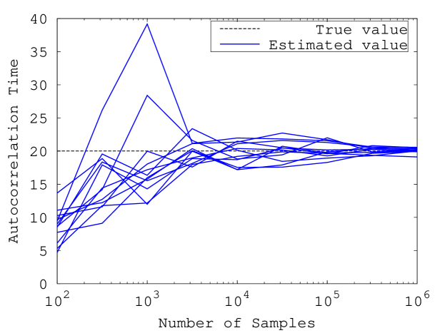
Figure 3: The estimated maximum autocorrelation time in the 1D Gaussian problem.

Table 1: The weights of the linear combination of the three observables with $a_{1}$ normalized to 1.

	$N=10^{3}$	$N=10^{4}$	$N=10^{5}$	$N=10^{6}$
$a_{1}$	-0.036	-0.008	0.003	0.010
$a_{2}$	0.972	1.024	1.008	0.994
$a_{3}$	1.000	1.000	1.000	1.000

4.2 An L-shaped mixture of two Gaussian distributions

Consider again the mixture of two Gaussians with target density given by eqn. (2) sampled with discrete Brownian dynamics with time step size $\Delta t=0.02$ and subsampled at time interval $0.1$ (every 5 points). The given observables are $q_{1}$ and $q_{2}$. Theoretically, $q_{1}$ should have larger autocorrelation time than $q_{2}$ for small $N$ while the chain remains in the horizontal leg of the ”L”, since the frequency is smaller in the direction of $q_{1}$ than it is in the direction of $q_{2}$. By the same reasoning, the weight for $q_{1}$ in the linear combination forming the maximizing observable should be greater than the weight for $q_{2}$, when $N$ is small. Due to symmetry, on the other hand, both auto-correlation times and the magnitudes of the weight for $q_{1}$ and $q_{2}$ should be equal when $N$ large.

Figure 4 shows ESS and $\tau$ of single observables and the maximizing observable. It can be seen that $\tau_{\max}$ is always greater than the larger $\tau$ of individual observables. As is discussed in previous section, this tells us that obtaining $\tau_{\max}$ is helpful for better convergence detection. Table 2 shows the weights of linear combinations for different sample sizes. The weighting obtained meets expectations, ultimately giving equal weight to $q_{1}$ and $q_{2}$.

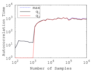
(a) Auto-correlation time

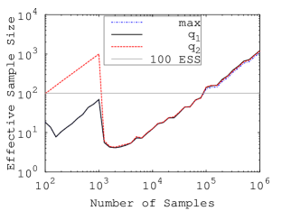
(b) Effective sample size

Figure 4: Effective sample size and autocorrelation time vs. number of samples in the L-shape mixture of Gaussians.

Table 2: The weights of the linear combination of the $q_{1}$ and $q_{2}$ with $a_{1}$ normalized to $1$.

	$N=10^{3}$	$N=10^{4}$	$N=10^{5}$	$N=10^{6}$
$a_{1}$	1.000	1.000	1.000	1.000
$a_{2}$	0.089	0.085	-1.207	-1.051

4.3 A one-node neural network

Consider the simplest Bayesian neural network regression model [1], having a single node in the hidden layer:

$$y\approx u(\mathbf{q};x)=q_{3}\tanh(q_{1}x+q_{2})+q_{4},$$

where $(x,y)$ represents a data point. Suppose a total of $100$ data points are given as shown by the large dots of Figure 5 (a). The posterior distribution is

$$-\log\rho(\mathbf{q})=\frac{1}{2}\beta\sum_{i=1}^{100}(y_{i}-u(\mathbf{q};x_{i}))^{2}+\frac{1}{2}\alpha\|\mathbf{q}\|^{2}+\mbox{const},$$

where $\beta=2.5$ and $\alpha=0.8$. Suppose the sampler is discretized Brownian dynamics with $\Delta t=0.01$, and let the Markov chain be obtained by subsampling the original trajectory at time interval $0.1$ (every 10 points). The given observables for finding the maximizing observable are the parameters of the model $q_{1}$, $q_{2}$, $q_{3}$ and $q_{4}$. The prediction for the first data point

$$\bar{u}(x_{1}):=\frac{1}{N}\sum_{i=1}^{N}u(\mathbf{q}_{i};x_{1})$$

is also examined as an example of an observable of interest.

Figure 5 (a) shows the overall prediction $\bar{u}(x)$ resulting from the regression model, and Figures 5 (b) and (c) show the trajectories of observables. It can be seen that when the sampling is insufficient, the prediction is inaccurate (the asymmetry implies only one mode is explored). It can also be seen that the maximizing observable makes many fewer transitions than $q_{1}$. This is because the maximizing observable tends to make the “hardest” moves, hence has longest autocorrelation time.

Figure 6 (a) and (b) show the ESS and $\tau$ for single observables and the maximizing observable. It can be seen that the ESS of the prediction $\bar{u}(x_{1})$ is obviously misleading for convergence detection, since it indicates sufficient sampling when $N\approx 100$. It can also be seen that the maximum $\tau$ is significantly larger than the longest $\tau$ of individual observables. This is a result of combining 4 observables linearly.

Figure 6 (c) shows the mean squared error of the regression converging when $N>2.0\times 10^{4}$. This coincides with the convergence of $\tau_{\max}$. On the other hand, the the $\tau$ for the prediction might suggest stopping far too early and the $\tau$ for $q_{1}$ might also be too optimistic.

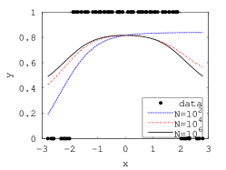
(a) The prediction

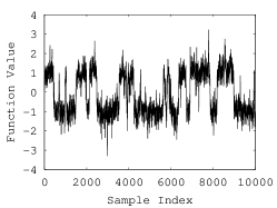
(b) Trajectory of $q_{1}$

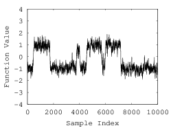
(c) Trajectory of $u_{\max}$

Figure 5: The resulting prediction and the trajectories of observables in the one-node neural network problem.

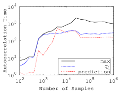
(a) $\tau$

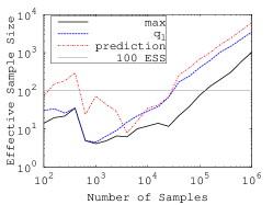
(b) ESS

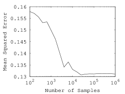
(c) MSE

Figure 6: Autocorrelation times, effective sample sizes, and the mean squared error for the one-node neural network model.

4.4 Logistic regression

Consider a Bayesian logistic regression model [3]. The logistic function maps a linear combination of features $\mathbf{x}$ to a probability:

$$\sigma(\mathbf{q};\mathbf{x})=1/(1+\exp(-\mathbf{q}^{\mathsf{T}}\mathbf{x})).$$

The posterior distribution is

$$-\log\rho(\mathbf{q})= \beta\sum_{i=1}^{n}(y_{i}\log(\sigma_{i})+(1-y_{i})\log(1-\sigma_{i}))$$

$$+\frac{1}{2}\alpha\|\mathbf{q}\|^{2}+\mbox{const.},$$

where $y_{i}$ is the class label of data example $i$, $\beta=1.0$, $\alpha=0.1$, and $n$ is the total number of data examples. When predicting the label of a given data example $\mathbf{x}$, use the average value

$$\bar{\sigma}(\mathbf{x})=\frac{1}{N}\sum_{i=1}^{N}\sigma(\mathbf{q}_{i};\mathbf{x})$$

over all samples. The label $t$ of a data example $\mathbf{x}$ is predicted to be $1$ if $\bar{\sigma}(\mathbf{x})\geq 0.5$ and $0$ if $\bar{\sigma}(\mathbf{x})<0.5$. For data, use the Australian Credit Approval dataset from the UCI machine learning data repository [9]. It contains 690 data examples and provides 15 features for each data example. Half of the examples in the dataset are extracted to form the training set, and the rest of them are in the testing set. The sampler is Brownian dynamics with $\Delta t=0.05$. This step size best balances computation cost and sampling accuracy (measured by the training error). As for the one-node neural network problem, the model parameters $q_{i}$ are used as observables for estimating $\tau_{\max}$ and the prediction for the first data point in the training set as an observable of interest.

Figure 7 shows $\tau$, the ESS, and the training/testing error in the logistic regression problem. The training error is defined as

$$err_{\mathrm{train}}=\frac{1}{n}\sum_{i=1}^{n}1_{t(\mathbf{x}_{i})\neq y_{i}}$$

The testing error is defined similarly except the data examples are from the testing set.

In practice, one may monitor convergence by observing the convergence of the training error. This approach, however, can be very expensive for large data sets. One has to evaluate the prediction function for all data examples. Instead, one might observe the convergence of observables such as the prediction function of a single data example or a single weight. But as is shown in the figure, it is risky to only observe one of them. Both the training and testing error do not converge until the number of samples exceeds $1000$, but both the prediction and the weight$q_{1}$ have an almost constant autocorrelation time equal to 1 (implying independent samples). This is obviously misleading. On the other hand, the maximizing observable does not show convergence until $N>1000$. This demonstrates that the maximzing observable is a more reliable indicator of convergence.

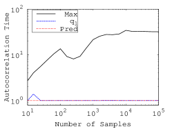
(a) $\tau$

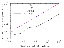
(b) ESS

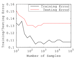
(c) Training error

Figure 7: The autocorrelation times, the effective sample sizes, and the training/testing error in the logistic regression problem.

5 Discussion and conclusions

There is considerable agreement on the importance of estimating the integrated autocorrelation time $\tau$. It is illustrated here and acknowledged by others that better estimates of $\tau$ are needed. Derived and presented here are computational methods based on estimating the greatest possible $\tau$, which for some problems give more reliable estimates at a cost that is only a small fraction of that required to generate the samples. The approach suggested here is quite general, and there are opportunities for refinement, for example, using better basis functions.

Appendix A Marginally Better Estimates of Integrated Autocorrelation Time

A.1 An optimal lag window

The autocorrelation function can be highly oscillatory, which would invalidate the method proposed here. To obtain a much more slowly varying function, use values based on doubling: $v_{i}=u(\mathbf{q}_{2i})+u(\mathbf{q}_{2i+1})$. In the case of a reversible sampler, this can be shown to yield a positive decreasing convex autocorrelation function [4, Sec. 3.3]. It is straightforward to show that the autocorrelation time of $u(\mathbf{q})$ can be recovered from that of $v$:

$$\tau_{u}=\frac{1}{2}\frac{C_{v}(0)}{C_{u}(0)}\tau_{v}.$$

A.1.1 Form of lag window

Assume the use of a lag window with $0\leq w(k)\leq 1$ and $w(k)$ nonincreasing. Assume that covariance estimates $C_{N}(k)$ satisfy

$$C_{N}(k)=C(k)+\sigma C(0)\eta_{k}$$

for some nonnegative value $\sigma$ where the $\eta_{k}$ are independent standard normally distributed random values. The estimated autocorrelation time is

$$\tau^{\mathrm{est}}=1+2\sum_{k=1}^{+\infty}w(k)\frac{c(k)+\sigma\eta_{k}}{1+\sigma\eta_{0}}$$

where $c(k)=C(k)/C(0)$ is the ACF and $w(k)=0$ for $k\geq M$. Assuming $\sigma\ll 1$, the error in the integrated autocorrelation time, to a first approximation, is

$$-2R+2\sigma\sum_{k=1}^{+\infty}w(k)\eta_{k}-2\sigma\eta_{0}\sum_{k=1}^{+\infty}w(k)c(k),$$

where

$$R=\sum_{k=1}^{+\infty}(1-w(k))c(k).$$

The expectation of the square of the error is

$$4R^{2}+4\sigma^{2}\sum_{k=1}^{+\infty}w(k)^{2}+4\sigma^{2}\left(\sum_{k=1}^{+\infty}w(k)c(k)\right)^{2},$$

which is minimized for a given value of $m$ if

$$w(k)=\frac{c(k)}{\sigma^{2}}\left(R-\sigma^{2}\sum_{k=1}^{+\infty}w(k)c(k)\right).$$ (4)

Note that, for small enough $\sigma$, the right-hand side is positive.

The ACF $c(k)$ is unknown, so, for the purpose of defining the lag window, it is suggested to use the specific model

$$C_{N}(k)=c_{0}\lambda^{k}+\sigma c_{0}\eta_{k},$$

where $\lambda$, $c_{0}$, and $\sigma$ are determined as in Section A.1.2 that follows. The goal is to capture the behavior of the tail of the ACF, which will be achieved by using enough points $M$ in the fitting. Then $c(k)=\lambda^{k}$, so $w(k)$ is proportional to $\lambda^{k}$, suggesting the choice

$$w(k)=\min\{1,\lambda^{k-m}\}$$ (5)

where $m$ is to be determined optimally.

Using the specific model for $C_{N}(k)$, the expectation of the error squared becomes

$$\frac{4c_{0}\lambda^{2}}{(1-\lambda^{2})^{2}}\left(\mu^{2}+\sigma^{2}(1+\lambda-\mu)^{2}\right)+\frac{4\sigma^{2}\log\mu}{\log\lambda}-\frac{4\sigma^{2}}{1-\lambda^{2}}$$

where $\mu=\lambda^{m}$. Differentiating with respect to $\mu$ and setting the result to zero leads to a quadratic equation for $\mu$, which can be shown to have a positive and negative root. If the positive root exceeds 1, this indicates that the sample size $N$ is not large enough.

A.1.2 Fitting the autocorrelation function

With residuals

$$r_{k}=c_{0}\lambda^{k}-C_{N}(k),$$

the parameters $c_{0}$ and $0<\lambda<1$ minimize $\sum_{k=0}^{M-1}r_{k}^{2}$. The value of $c_{0}$ that minimizes this must satisfy

$$\sum_{k=0}^{M-1}\lambda^{k}r_{k}=0,$$

whence $c_{0}={Q(\lambda)}/{P(\lambda)}$, where

$$P(\lambda)=\sum_{k=0}^{M-1}\lambda^{2k}\mbox{ and }Q(\lambda)=\sum_{k=0}^{M-1}C_{N}(k)\lambda^{k}.$$

Substituting this into the objective function gives

$$\sum_{k=0}^{M-1}r_{k}^{2}=-\frac{Q(\lambda)^{2}}{P(\lambda)}+\sum_{k=0}^{M-1}c(k)^{2}.$$ (6)

The optimal value of $\lambda$ is obtained by minimizing this rational function. (One can use golden section search beginning with the interval $[0,1]$. We used bisection applied to the gradient.) The ML estimate of the standard deviation $\sigma$ of the noise is obtained from the RMS of the resulting residual.

One can simply use the exponential model for the tail $\sum_{k=M}^{N-1}w(k)C_{N}(k)$ of $\tau^{\mathrm{est}}$.

A.2 A comparison with the lag window of acor

Figure 8 shows the estimated $\tau$’s of $H_{1}$ and $H_{1}+H_{2}+H_{3}$ as well as $\tau_{\max}$. It can be seen that when $N$ is small, both methods underestimate $\tau$, but the new one gives larger estimates. When $N$ is large, both methods converge to the true value, and the new method has a smaller variance. Overall, the proposed lag window is more reliable than acor.

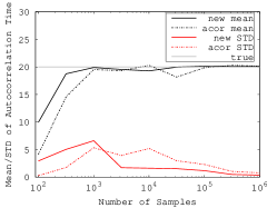
(a) $H_{1}$

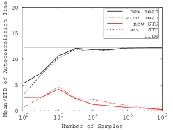
(b) $H_{1}+H_{2}+H_{3}$

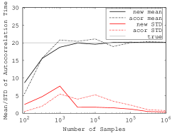
(c) $\tau_{\max}$

Figure 8: Estimated $\tau$ and $\tau_{\max}$ by the new lag window and acor for the 1D standard Gaussian.

A.3 The lag window for extremely small ESS

It might be difficult to get a good lag window when the number of samples is extremely insufficient. Figure 9 shows the lag window obtained by the new method and acor in the one-node neural network problem. For acor, the lag window obviously contains not enough data. And for the proposed method, it contains perhaps too much data since some of the data is already in the negative value range due to statistical error. The noise for the auto-correlation function estimator is highly correlated when $\tau$ is large. In this example, the effective sample size is less than 10. In such cases, $\tau$ may be underestimated by both methods.

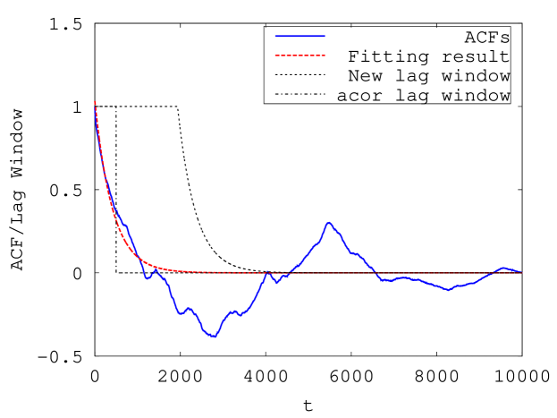
Figure 9: An example of ACF and lag window for the one-node neural network problem.

References

- [1] C. M. Bishop. Neural Network for Pattern Recognition. Clarendon Press, 1996.
- [2] S. Duane, A. D. Kennedy, B. J. Pendleton, and D. Roweth. Hybrid Monte Carlo. Phys. Rev. B, 195:216–222, 1987.
- [3] A. Gelman, J. B. Carlin, H. S. Stern, and D. B. Rubin. Bayesian Data Analysis. New York: Chapman and Hall, 2004.
- [4] C. J. Geyer. Practical Markov chain Monte Carlo. Stat. Sci., 7:473–511, 1992.
- [5] J. Goodman. Acor, statistical analysis of a time series, Spring 2009.
- [6] A. M. Horowitz. A generalized guided Monte-Carlo algorithm. Phys. Lett. B, 268:247–252, 1991.
- [7] B. Leimkuhler and C. Matthews. Rational construction of stochastic numerical methods for molecular sampling. Appl. Math. Res. Express, pages 34–56, 2013.
- [8] B. Leimkuhler, C. Matthews, and G. Stoltz. The computation of averages from equilibrium and nonequilibrium Langevin molecular dynamics. IMA J. Numer. Anal., 36:13–79, 2016.
- [9] M. Lichman. UCI machine learning repository, 2013.
- [10] N. Metropolis, A. Rosenbluth, M. Rosenbluth, A. Teller, and E. Teller. Equation of state calculations by fast computing machines. J. Chem. Phys., 21:1087–1092, 1953.
- [11] M. B. Priestly. Spectral Analysis and Time Series. Academic Press, 1981.
- [12] H. Risken. The Fokker-Planck Equation. Springer, 1996.
- [13] G. O. Roberts and R. L. Tweedie. Exponential convergence of Langevin diffusions and their discrete approximations. Bernoulli, 2:341–363, 1996.
- [14] C. Schütte and W. Huisinga. Biomolecular conformations as metastable sets of Markov chain. Proceedings of the 38th Annual Allerton Conference on Communication, Control and Computing,, pages 1106–1115, 2000.
- [15] A. Sokal. Monte Carlo methods in statistical mechanics: Foundations and new algorithms. In C. DeWitt-Morette, P. Cartier, and A. Folacci, editors, Functional Integration: Basics and Applications, pages 131–192. Springer US, Boston, MA, 1997.
- [16] G. Vilmart. Postprocessed integrators for the high order integration of ergodic SDEs. SIAM J. Sci. Comput., 37:A201–A220, 2015.