Spectrum of the open QCD flux tube and its effective string description I: 3d static potential in SU($N=2,3$)

Abstract

We perform a high precision measurement of the static $q\bar{q}$ potential in three-dimensional $\text{SU}(N)$ gauge theory with $N=2,3$ and compare the results to the potential obtained from the effective string theory. In particular, we show that the exponent of the leading order correction in $1/R$ is 4, as predicted, and obtain accurate results for the continuum limits of the string tension and the non-universal boundary coefficient $\bar{b}_{2}$, including an extensive analysis of all types of systematic uncertainties. We find that the magnitude of $\bar{b}_{2}$ decreases with increasing $N$, leading to the possibility of a vanishing $\bar{b}_{2}$ in the large $N$ limit. In the standard form of the effective string theory possible massive modes and the presence of a rigidity term are usually not considered, even though they might give a contribution to the energy levels. To investigate the effect of these terms, we perform a second analysis, including these contributions. We find that the associated expression for the potential also provides a good description of the data. The resulting continuum values for $\bar{b}_{2}$ are about a factor of 2 smaller than in the standard analysis, due to contaminations from an additional $1/R^{4}$ term. However, $\bar{b}_{2}$ shows a similar decrease in magnitude with increasing $N$. In the course of this extended analysis we also obtain continuum results for the masses appearing in the additional terms and we find that they are around twice as large as the square root of the string tension in the continuum and compatible between SU(2) and SU(3) gauge theory. In the follow up papers we will extend our investigations to the large $N$ limit and excited states of the open flux tube.

1 Introduction

Flux tube formation between quark $q$ and antiquark $\bar{q}$ provides a possible mechanism for quark confinement and has been verified in simulations of lattice QCD (e.g. Bali:1994de ). While the microscopic origin of the formation of the flux tube is still debated, it is common consensus that the long distance properties, in particular the spectrum, are well described by an effective string theory (EST). The EST is a two dimensional effective field theory for the Goldstone bosons associated with the breaking of translational symmetry, the quantised transversal oscillation modes. While the basic properties of the theory are known for a long time Goto:1971ce ; Goddard:1973qh ; Nambu:1978bd ; Luscher:1980fr ; Polyakov:1980ca a number of features have only been elucidated in the past decade Luscher:2004ib ; Aharony:2009gg ; Aharony:2010db ; Aharony:2010cx ; Aharony:2011ga ; Billo:2012da ; Dubovsky:2012sh ; Dubovsky:2012wk ; Aharony:2013ipa ; Caselle:2013dra ; Dubovsky:2014fma ; Caselle:2014eka . In particular, it has been clarified Dubovsky:2012wk that the leading order spectrum agrees with the light cone quantisation Arvis:1983fp of the Nambu-Goto string theory (LC spectrum, eq. (7)) and the corrections to the LC spectrum have been computed up to $O(R^{-5})$ Aharony:2010db ; Aharony:2011ga ; Caselle:2013dra , where $R$ is the distance between quark and antiquark. For more details and a recent review see Brandt:2016xsp .

The predictions of the EST can be compared to lattice results for the excitation spectrum of the flux tube and good agreement has typically been found, proceeding down to $q\bar{q}$ separations where the EST is not expected to be reliable (for a compilation of results see Brandt:2016xsp ). In particular, the EST predicts a boundary correction of $O(R^{-4})$ with a free and, presumably, non-universal coefficient $\bar{b}_{2}$. This coefficient has first been extracted from the excited states in 3d SU(2) Brandt:2010bw and later from the groundstate in 3d $Z_{2}$ Billo:2012da and SU($N=2,3$) Brandt:2013eua gauge theory for a number of different lattice spacings. Indeed, strong evidence for a non-universal behaviour has been found. The good agreement down to small values of $R$ is surprising, given that the flux tube profile only agrees with the EST starting from around 1.0 fm, at least Bali:1994de ; Gliozzi:2010zv ; Cardoso:2013lla ; Caselle:2016mqu . A possible explanation could be that the flux tube consists of a solid, vortex-like core whose fluctuations are governed by the EST. This would explain the good agreement of the profile with the associated exponential decay, e.g. Cea:2012qw ; Cea:2014uja ; Caselle:2016mqu , rather then with the Gaussian profile predicted by the EST Luscher:1980iy ; Caselle:1995fh , while leaving the spectrum untouched to leading order.  In fact, it has been found Cardoso:2013lla that the profile can be analysed using a convolution of the EST and vortex profiles, which would indicate that the flux tube shares features of both.

One can expect that a particular class of corrections to the EST might show up as massive modes on the worldsheet. Indeed, candidates for states receiving contributions from massive modes have been seen in 4d $\text{SU}(N)$ gauge theories Morningstar:1998da ; Juge:2002br ; Juge:2004xr ; Athenodorou:2010cs and the results for closed strings Athenodorou:2010cs are in good agreement with the energy levels obtained by including a massive pseudoscalar particle on the worldsheet known as the worldsheet axion Dubovsky:2013gi ; Dubovsky:2014fma . Recently, the behaviour of the mass of the worldsheet axion for $N\to\infty$ has been investigated Athenodorou:2017cmw and a finite result has been found in this limit. It is interesting to note that possible massive modes are only seen in 4d, which might be due to the fact that the topological coupling term associated with the worldsheet axion only exists for $d>3$ (see section 2.3). Consequentially, any massive modes in 3d can only couple via terms contributing to higher orders in the derivative expansion or via vertices including more than one massive field. In this case results at intermediate distances are potentially less affected and the massive modes appear as quasi-free modes on the worldsheet.

Apart from the contribution of massive modes, there could also be contributions from rigidity. The associated term satisfies the symmetry constraints of the theory and naturally turns up in cases where the EST can be derived from a vortex solution of the underlying field theory Forster:1974ga ; Gervais:1974db ; Lee:1993ty ; Orland:1994qt ; Sato:1994vz ; Akhmedov:1995mw . While the contributions due to this term start at higher orders in the derivative expansion of the EST (and thus should be negligible up to $O(R^{-7})$, at least), it has been found, using zeta function regularisation, that its non-perturbative (in the sense of the $1/R$ expansion) contribution cannot be expanded systematically in $R^{-1}$. It thus leads to contamination at all orders which are, however, exponentially suppressed for large values of $R$ Polyakov:1986cs ; German:1989vk ; Ambjorn:2014rwa ; Caselle:2014eka . In fact, the leading order contribution is formally equivalent to the contribution of a free massive particle, as discussed in section 2.3.

In this series of papers we will investigate in detail the agreement of the spectrum of the open flux tube in $\text{SU}(N)$ gauge theories with the predictions from the EST. Particular emphasis lies on the reliable extraction of the boundary coefficient $\bar{b}_{2}$ from the static potential and its continuum extrapolation. In this context it is also important to control the higher order corrections. For the case that the other corrections are regular corrections that are part of the derivative expansion, the next term would be of $O(R^{-\gamma})$ with $\gamma\geq 6$. Such corrections are comparably easy to disentangle from the boundary term. If, on the other hand, there are contributions from the rigidity term, or equivalently from massive modes, those can contaminate the extraction of $\bar{b}_{2}$ German:1989vk ; Ambjorn:2014rwa ; Caselle:2014eka . We will see that we cannot exclude the latter possibility, but we can show that in a certain range of distances the exponent of the correction term with respect to the LC spectrum is indeed 4 and it is not well described by the additional terms alone. Since we cannot exclude the contamination of $\bar{b}_{2}$, we carry out two independent analyses, excluding and including the rigidity/massive mode contributions. Eventually we are interested in the large $N$ limit of the non-universal contributions. In particular, there is hope that some of the non-universal parameters can be used to constrain the possible holographic backgrounds and eventually help to find the holographic dual of large $N$ Yang-Mills theory.

In this first paper of the series we will introduce the methods that we use to analyse the potential in $\text{SU}(N)$ gauge theory. However, we focus only on results for $N=2$ and 3 in three dimensions and leave the extraction of the results for $N>3$ and the extrapolation $N\to\infty$ for the next paper in the series. In follow up papers we plan to consider excited states, extending the studies from Brandt:2009tc ; Brandt:2010bw , and the four dimensional theory. The paper is organised as follows: In the next section we briefly discuss the relevant predictions and properties of the EST and its limitations. The consequent section 3 is devoted to the basic analysis of the lattice data for the static potential. In particular, we perform a reliable extraction of the Sommer parameter and the string tension and show the leading correction to the LC spectrum is indeed of $O(R^{-4})$. In sections 4 and 5 we extract $\bar{b}_{2}$ excluding/including massive mode contributions, respectively. Section 6 provides the summary and discussion of the main results of the two analyses and we conclude in section 7. The details of the lattice simulations are presented in appendix A and we discuss the control of systematic uncertainties in appendix B.

2 Effective string theory predictions

We start by discussing the properties of the EST, focusing on the relevant aspects for the present study. For more detailed reviews we refer to Aharony:2013ipa ; Brandt:2016xsp .

2.1 Effective string theory and its limitations

The EST is the low energy effective field theory (EFT) describing a single, stable, non-interacting flux tube. Here we will focus on the case of a flux tube stretched between two sources in the fundamental representation (quark and antiquark), but one can also study the hypothetical case of a closed flux tube wrapping around a compactified dimension. The presence of the flux tube breaks translational invariance in the transverse directions, leading to $d-2$ Goldstone bosons (GBs), the quantised transverse oscillation modes. For brevity we will consider the string of length $R$ to reside in the $(x^{0},x^{1})$-plane ($x^{0}$ being the temporal direction) with endpoints located at $x^{1}=0$ and $R$. Then one can parametrise the fluctuation field by $X^{\mu}(x^{\alpha})=(x^{\alpha},\,X^{i}(x^{\alpha}))$, where $\alpha=0,1$, $i=2,\ldots,d$ and the $X^{i}$ are the GBs of the EST. The action up to 6 derivatives order has been derived in Aharony:2009gg ; Aharony:2010cx ; Billo:2012da together with the constraints for the coefficients (the result for the coefficient $c_{4}$ has been clarified in Dubovsky:2012wk ). Here we will write down the action in the static gauge (instead of the diffeomorphism invariant form discussed in Aharony:2013ipa ; Brandt:2016xsp ) and in Minkowski space for simplicity. Since we are considering an open string the action consists of two parts,

$$S_{\rm EST}=S_{\rm c}+S_{\rm b}\,,$$ (1)

where $S_{\rm c}$ is the bulk action,

$$\begin{array}[]{rcl}\displaystyle S_{\rm c}&\displaystyle=\int_{\mathcal{M}}d^{2}x&\displaystyle\big{[}-\sigma-\frac{\sigma}{2}\,\partial_{\alpha}X^{i}\partial^{\alpha}X^{i}+c_{2}(\partial_{\alpha}X^{i}\partial^{\alpha}X^{i})^{2}+c_{3}(\partial_{\alpha}X^{i}\partial_{\beta}X^{i})^{2}\vspace*{2mm}\\ &&\displaystyle\>\>\>+c_{4}(\partial_{\alpha}\partial_{\beta}X^{i}\partial^{\alpha}\partial^{\beta}X^{i})(\partial_{\gamma}X^{j}\partial^{\gamma}X^{j})+c_{5}(\partial_{\alpha}X^{i}\partial^{\alpha}X^{i})^{3}\vspace*{2mm}\\ &&\displaystyle\>\>\>+c_{6}(\partial_{\alpha}X^{i}\partial^{\alpha}X^{i})(\partial_{\beta}X^{j}\partial_{\gamma}X^{j})^{2}+\dots\big{]},\end{array}$$ (2)

where the integral runs over the worldsheet $\mathcal{M}$ of the flux tube, and $S_{\rm b}$ the boundary action

$$S_{\rm b}=\int_{\partial\mathcal{M}}d^{2}x\>\big{[}\mu+b_{1}\partial_{1}X^{i}\partial_{1}X^{i}\!+b_{2}\partial_{0}\partial_{1}X^{i}\partial_{0}\partial_{1}X^{i}+b_{3}(\partial_{1}X^{i}\partial_{1}X^{i})^{2}\dots\big{]},$$ (3)

where the integral runs over the woldsheet boundary $\partial\mathcal{M}$.

The coefficients in eqs. (2) and (3) are constrained by the residual symmetries of the effective field theory, which for the EST is Lorentz symmetry. The results for the coefficients are Aharony:2009gg ; Aharony:2010cx ; Billo:2012da ; Dubovsky:2012wk

$$c_{2}=-\frac{\sigma}{8}\,,\quad c_{3}=\frac{\sigma}{4}\,,\quad c_{4}=0\,,\quad c_{5}=\frac{\sigma}{16}\,,\quad c_{6}=-\frac{\sigma}{8}\,,\quad b_{1}=0\quad\text{and}\quad b_{3}=0\,,$$ (4)

while $b_{2}$ remains unconstrained and thus represents the first subleading low energy constant not fixed in terms of $\sigma$. In the next section we will discuss the spectrum which follows from the effective action. Note, that $b_{2}$ is a dimensionfull quantity, so that, for the purpose of lattice simulations and the associated continuum limit, it makes sense to introduce the dimensionless coupling

$$\bar{b}_{2}=\sqrt{\sigma^{3}}b_{2}\,,$$ (5)

which we will use from now on.

On top of the terms in eq. (1), there is one more class of terms allowed within the EST, constructed from powers of the extrinsic curvature Aharony:2013ipa ; Caselle:2014eka . The leading order term is known as the rigidity term and has first been proposed by Polyakov Polyakov:1996nc . It also turns up in those cases where vortex solutions could be constructed from the underlying microscopic theory Forster:1974ga ; Gervais:1974db ; Lee:1993ty ; Orland:1994qt ; Sato:1994vz ; Akhmedov:1995mw . In this sense, the presence of rigidity terms can be seen as evidence of vortex contributions to the EST energies. Rigidity contributions to energy levels start at higher orders in the perturbative expansion, but it has been found that it leads to a non-perturbative contributions to the energy levels in zeta-function regularisation Braaten:1986bz ; German:1989tr ; Caselle:2014eka . However, as pointed out in Dubovsky:2012sh , this regularisation scheme does not preserve the non-linear Lorentz symmetry of the EST, leading to possible counterterms that need to be taken into account. It is thus mandatory to crosscheck this result using a regularisation scheme which preserves Lorentz invariance. In this paper we will use the result as presented in Caselle:2014eka , which we summarise and discuss in more detail in section 2.3.

The EST is expected to break down at the point where the energy of the fluctuation modes reaches the QCD scale $\Lambda_{\rm QCD}\approx\sqrt{\sigma}$. The energy of the modes is of the order $1/R$, meaning that the EST is expected to break down for

$$\sqrt{\sigma}R\lesssim 1\,.$$ (6)

Owing to the derivative expansion in eqs. (2) and (3) this makes sense, since each derivative is of the order of one unit of momentum of the degrees of freedom, $\partial\sim p\sim 1/R$, so that the EST corresponds to an expansion in $(\sqrt{\sigma}R)^{-1}$ which is expected to break down when eq. (6) is fulfilled. On top of this, there are also several processes that are allowed in the microscopic theory, but are not accounted for within the EST. Among them is the emission of glueballs. If those are on-shell, the emitting state has to be an excited state with $E\geq E^{\prime}+m_{G}$, where $E^{\prime}$ is the state it decays to and $m_{G}$ is the mass of the lightest glueball with appropriate quantum numbers. Consequently, such a process can only appear for excited states with $E_{n}>E_{0}+m_{G}$, where $E_{0}$ is the groundstate. On top of this on-shell emission, there can also be virtual glueball exchange. This process will always be present (at finite $N$) and leads to corrections of unknown size. These meson-glueball interactions and mixings are suppressed with increasing $N$ and vanish in the $N=\infty$ limit (e.g. Lucini:2012gg ). Furthermore, within the EST the string is not allowed to develop knots or to intersect with itself, which would correspond to handles on the worldsheet. In addition, the flux tube is likely to have an intrinsic width, allowing for inner excitations, contributing in the form of massive excitations on the worldsheet which have to be added to the EST. We will discuss these additional modes and their possible contributions in section 2.3.

In general, the EST only describes a single non-interacting and stable string. We would like to emphasise that this is not the case realised for the flux tube in QCD, which can break due to the creation of a light $q\bar{q}$ pair from the vacuum. Furthermore, the quarks are taken to be static, meaning that one takes the limit of infinitely heavy quarks. The effect of finite quark masses can be included using non-relativistic effective field theories of QCD Brambilla:2000gk ; Pineda:2000sz ; Brambilla:2003mu ; Brambilla:2004jw , for instance (see Brambilla:2014eaa for a recent evaluation of the $1/m^{2}$ corrections to the potential using the EST predictions). In this paper, however, we will focus on pure gauge theory, where effects owing to finite quark masses are absent and the EST holds up to the limitations discussed above.

We close this section by noting that one possibility for an extension of the standard EST to include the effect of possible internal excitation or external influences on the flux tube is to view them as ‘defects’ on the worldsheet Andreev:2012mc ; Andreev:2012hw . Here a defect is a place on the string where the derivatives of the coordinates are discontinuous. The associated effect has been worked out for the potential and found to be in reasonable agreement with observed anomalous states in four dimensions Andreev:2012hw .

2.2 Spectrum of the open string and boundary corrections

We will now discuss the spectrum that follows from the action (1). The constraints in eq. (4) for the coefficients set $c_{2}$ to $c_{6}$ to the values they obtain in the NG theory. Consequently, one can expect that the leading order spectrum is equivalent to the NG one, up to the corrections due to the boundary term proportional to $\bar{b}_{2}$. This expectation is corroborated by the formulation of the EST in diffeomorphism invariant form Aharony:2013ipa , where the full NG action appears as the leading order term in the action. The main question thus concerns the spectrum following from the NG action in $d$ dimensions. For $d=26$ and $d=3$ the exact spectrum is known from the light cone (LC) quantisation and takes the form Arvis:1983fp

$$E^{\rm LC}_{n}(R)=\sigma\>R\>\sqrt{1+\frac{2\pi}{\sigma\>R^{2}}\>\left(n-\frac{1}{24}\>(d-2)\right)}\;.$$ (7)

Note, that we only consider open strings, so that $n$ denotes the number of phonon excitations and as such labels the excitation level. The first few excited states in terms of phonon creation operators $\alpha^{i}_{-m}$ (for phonon momentum $m$) are listed in table 1. However, the LC quantisation breaks Lorentz invariance explicitly so that, away from $d=26$ and $d=3$, counterterms are necessary for a consistent quantisation. The first counterterm is proportional to the $c_{4}$ term in eq. (2) with a coefficient Dubovsky:2012sh ; Dubovsky:2014fma

$$\tilde{c}_{4}=-\frac{d-26}{192\pi}\,.$$ (8)

Thus, the first correction in the bulk action to the LC spectrum appears at order $R^{-5}$, but, since the NG action only contains one free parameter, the correction is universal.

energy	$|n,l\big{\rangle}$	representation		$B_{n}^{l}$	$C_{n}^{l}$
$E_{0}$	$|0\big{\rangle}$	$\mathtt{1}|0\big{\rangle}$	scalar	0	0
$E_{1}$	$|1\big{\rangle}$	$\alpha^{i}_{-1}|0\big{\rangle}$	vector	4	$d-3$
$E_{2,1}$	$|2,1\big{\rangle}$	$\alpha^{i}_{-1}\alpha^{i}_{-1}|0\big{\rangle}$	scalar	8	0
$E_{2,2}$	$|2,2\big{\rangle}$	$\alpha^{i}_{-2}|0\big{\rangle}$	vector	32	$16(d-3)$
$E_{2,3}$	$|2,3\big{\rangle}$	$\big{(}\alpha^{i}_{-1}\alpha^{j}_{-1}-\frac{\delta^{ij}}{d-2}\alpha^{i}_{-1}\alpha^{i}_{-1}\big{)}|0\big{\rangle}$	sym. tracel. tensor	8	$4(d-2)$

Table 1: String states in the lowest three energy levels and their representation in terms of creation operators $\alpha_{m}$ in the Fock space together with their representation with respect to SO($d-2$). We also list the associated values for the numbers $B_{n}^{l}$ and $C_{n}^{l}$ appearing in eq. (10). ‘sym. tracel.’ for the state $|2,3\big{\rangle}$ stands for ‘symmetric traceless’.

One might thus wonder whether the square root formula in eq. (7) should be taken as the starting point of the expansion, or whether it is rather its expansion in orders of $R^{-1}$. In fact, this has been one of the biggest puzzles associated with the EST in the past decades. Lattice data (see Brandt:2016xsp for a compilation) show excellent agreement with the full square root formula even down to values of $R$ where its expansion breaks down. It thus has been conjectured that it should be the full formula which provides a reasonable starting point (e.g. Athenodorou:2010cs ; Brandt:2010bw ). The discussion above agrees with this conjecture in the sense that the LC spectrum can schematically be written as Dubovsky:2012sh

$$E^{\rm LC}_{n}(R)=E^{\rm NG}_{n}(R)-{\rm counterterms}\,.$$ (9)

Consequently, it will always be the full square root formula which appears when we solve the above equation for $E^{\rm NG}_{n}$. Furthermore, an analysis using the machinery of the Thermodynamic Bethe Ansatz (TBA) shows, that the leading order $S$-matrix is integrable, leading to energies given by the full square root formula Dubovsky:2012sh ; Dubovsky:2014fma . Note, that the boundary term can also be included in this TBA analysis Caselle:2013dra .

Following the above discussion and the corrections to the LC spectrum computed in Aharony:2010db ; Aharony:2011ga the spectrum up to $O(R^{-5})$ is thus given by

$$E^{\rm EST}_{n,l}(R)=E^{\rm LC}_{n}(R)-\bar{b}_{2}\frac{\pi^{3}}{\sqrt{\sigma^{3}}R^{4}}\Big{(}B_{n}^{l}+\frac{d-2}{60}\Big{)}-\frac{\pi^{3}(d-26)}{48\sigma^{2}R^{5}}C_{n}^{l}+O(R^{-\xi})\,,$$ (10)

where we have inserted the dimensionless coupling $\bar{b}_{2}$ introduced in the previous section. $B_{n}^{l}$ and $C_{n}^{l}$ are dimensionless coefficients tabulated in table 1. They depend on the representation of the state with respect to rotations around the string axis, transformations of $X^{i}$ with elements of SO($d-2$), and thus lift the degeneracies of the LC spectrum. Note once more, that $C_{n}^{l}$ vanishes identically for $d=3$ since the state $|2,3\big{\rangle}$ does not exist in this case. This can also be seen from the associated term in the EST action, the $c_{4}$ term in eq. (2), which is trivial for $d=3$. The next correction term to the LC energies can be expected to appear with an exponent $\xi=6$ or $\xi=7$, depending on whether the next correction originates from another boundary term (which will generically be the case if the associated coefficient does not vanish identically due to symmetry) or a bulk term.

2.3 Beyond the standard EST: massive modes and rigidity term

As mentioned already in the introduction and in section 2.1, there is also another class of terms allowed within the EST containing the extrinsic curvature. The leading order term of this type is known as the rigidity term, whose presence has first been found in Polyakov:1986cs . In terms of the derivative expansion the contributions of the rigidity term start at 8th derivative order, but the presence of this term in the action can give a non-perturbative contribution to the potential Klassen:1990dx ; Nesterenko:1997ku ; Caselle:2014eka . Including the first two terms from the bulk action, eq. (2), together with the leading order contribution from the rigidity term and evaluating the resulting Gaussian integral leads to a Euclidean potential of the form (for the details see Caselle:2014eka )

$$V(R)=\lim_{T\to\infty}\Big{\{}\sigma R+\frac{1}{2T}\log\Big{[}\det\big{(}-\Delta\big{)}\,\det\Big{(}1-\frac{\Delta}{m^{2}}\Big{)}\Big{]}\Big{\}},$$ (11)

where T is a finite temporal extent of the spacetime, $\Delta$ is the 2d Laplace operator, and we have introduced the mass

$$m=\sqrt{\sigma/2\alpha}\,.$$ (12)

The first determinant is the one resulting from a free massless boson field, leading to the Coulombic term within the EST, first computed by Lüscher Luscher:1980ac , while the second is reminiscent of the one of a free boson field with mass parameter $m$.

At this point it is important to stress that the contribution of the rigidity term resembles that of a massive excitation on the world sheet in Euclidean spacetime. However, the above result is only the leading order result, originating from the Gaussian part of the rigidity action. Higher order contributions will potentially spoil this equivalence. Nonetheless, at this order the two types of contributions cannot be disentangled.

Using zeta-function regularisation, the determinant of the massive boson in eq. (11) leads to a leading order term in the potential of the form Klassen:1990dx ; Nesterenko:1997ku ; Caselle:2014eka

$$V^{\rm rig}_{0}(R)=-\frac{m}{2\pi}\sum_{k=1}^{\infty}\frac{K_{1}(2kmR)}{k}\,,$$ (13)

which appears on top of the leading order Coulomb term originating from the massless determinant. Note, that the result has been obtained in zeta-function regularisation which breaks Lorentz invariance explicitly. Owing to the discussion in section 2.1 this means that one has to care for the inclusion of potential higher order counterterms in the action to obtain the correct result. The higher order terms in the action can be included perturbatively German:1989vk ; Caselle:2014eka , leading to the additional term Braaten:1986bz ; German:1989vk

$$V^{\rm rig}_{1}(R)=-\frac{(d-2)(d-10)\pi^{2}}{3840m\sigma R^{4}}\,,$$ (14)

which contaminates the $R^{-4}$ boundary term from eq. (10). Naively we expect a similar term in the presence of a free boson on the worldsheet.

To assess the effect of the term $V^{\rm rig}_{0}$ it is instructive to consider the two different limits with respect to the EST. First, let us consider the large $R$ limit, so that $mR\gg 1$. In this case the dominating contribution comes from the term in the sum with $k=1$, which gives a leading order contribution of the form Caselle:2014eka

$$V^{\rm rig}_{0}(R)\approx-\sqrt{\frac{m}{16\pi R}}e^{-2mR}\,.$$ (15)

Consequently, $V^{\rm rig}_{0}$ will be exponentially suppressed with respect to all other terms in the EST, so that it can only give a relevant contribution at intermediate or small values of $R$ for a given mass $m$. Next, let us consider the region of small $mR<\pi$. In this case one obtains Caselle:2014eka (keeping only the terms relevant for $R\to 0$)

$$V^{\rm rig}_{0}(R)\approx-\frac{\pi}{24R}+\frac{m^{2}R}{4\pi}\ln\Big{(}\frac{mR}{2\pi}\Big{)}+m\cdot O(mR)\,.$$ (16)

Thus, for small distances the rigidity term leads to another Coulombic term, doubling the standard Lüscher term within the EST. What is particularly important is the fact that in some intermediate regime (which, for not too large values of $m$, will still be within the validity region of $mR<\pi$ expansion) the Coulombic term will dominate over the $R^{-4}$ correction (while the logarithm is already negative). Consequently, we expect a negative Coulombic correction to the LC energy levels in some regime before seeing an $R^{-4}$ increase for $R\to 0$ if the $\bar{b}_{2}$ term is absent.

As a remark, we would like to stress that the above computation only applies to the potential. The modification of the excited energy levels due to the rigidity term are still unknown. For the purpose of this paper we will only need the potential, but a distinction between the boundary corrections and the rigidity term is notoriously difficult in this case. It would be very interesting to get a result for the associated modification of excited states. The hope is, that for the excited states the predictions including the massive modes is incompatible with the splittings between the energy levels, so that one can distinguish between the cases with or without massive mode contributions. In particular, it has been found in Brandt:2010bw that the splitting of the first few excitations is well described by the boundary term, which could be different when massive modes are included.

In the presence of additional massive bosonic degrees of freedom the presence of terms proportional to the extrinsic curvature also allows for a topological coupling term between the boson field and the GBs, proportional to the mode number Dubovsky:2013gi ; Dubovsky:2014fma  . Consequently, since the boson couples to the worldsheet analogue of the $\theta$-term, the boson can naturally be referred to as the worldsheet axion Dubovsky:2013gi . The action for the worldsheet axion can then be written as Dubovsky:2014fma

$$S_{\rm a}=\int_{\mathcal{M}}\sqrt{-h}\Big{(}-\frac{1}{2}\nabla_{\alpha}\phi\nabla^{\alpha}\phi-\frac{1}{2}m^{2}\phi^{2}-\frac{\gamma}{8\pi}\phi\,\epsilon_{ij}\epsilon^{\alpha\beta}K_{\alpha\gamma}^{i}K_{\beta}^{\gamma i}+\ldots\Big{)},$$ (17)

where $\nabla$ is the covariant derivative with respect to the induced metric $h^{\alpha\beta}=\partial^{\alpha}X\partial^{\beta}X$. To leading order, i.e. up to coupling terms of the form $\phi\partial_{\alpha}\partial_{\beta}\phi h^{\alpha\beta}$ and higher orders, $\nabla^{\alpha}$ can be replaced by $\partial^{\alpha}$. The associated leading order spectrum has been computed with the TBA method for closed strings in Dubovsky:2013gi ; Dubovsky:2014fma and has been found to be consistent with states showing an anomalously slow approach to the LC energies in the spectrum of the closed flux tube for $d=4$ Athenodorou:2010cs . Note that the topological coupling term in eq. (17) is only present for $d>3$, which could be a reason why no anomalous states have been observed in the 3d flux tube spectrum. In 3d massive modes appear as free bosons up to the coupling terms mentioned above. It would be interesting to include those coupling terms in a computation of the energy levels to check their influence on the spectrum.

In the following we will always denote the contributions discussed in this section as the contributions from “massive modes” for brevity. We would like to emphasise, however, that strictly speaking we can only compare our results to those obtained from the rigidity term, or from the leading order contribution, neglecting any direct couplings, of a massive boson on the worldsheet. Whether direct coupling terms are indeed negligible is an open question, which we cannot answer in the course of this study.

2.4 EST and gauge/gravity duality

We close the discussion of the EST with the remark that the EST action can potentially be computed (e.g. Aharony:2009gg and references therein) from the original 10d fundamental string theory appearing in a generalisation of the AdS/CFT correspondence for large $N$ gauge theories Maldacena:1997re ; Gubser:1998bc ; Witten:1998qj . For recent computations of properties of the flux tube in this framework see Kol:2010fq ; Vyas:2010wg ; Vyas:2012dg ; Giataganas:2015yaa . Consequently, constraining the possible terms and their couplings in the EST action could allow to constrain the fundamental string theory relevant for Yang-Mills theory.

In particular, in such cases where the background in the fundamental string theory is weakly curved, the additional bosonic and fermionic degrees of freedom (e.g. the additional coordinate fields in the directions transverse to the gauge theory plane and the supersymmetry partners of the bosonic fields) can be integrated out perturbatively. This has been done for closed strings and a special class of backgrounds in Aharony:2009gg and the resulting terms have been found to agree with the terms appearing in the EST bulk action, eq. (2). Furthermore, in Aharony:2010cx it has been shown that the same class of backgrounds considered for an open string ending on two infinitely stretched $D$-branes leads to the boundary term proportional to $\bar{b}_{2}$ in eq. (3). In terms of the masses of the additional bosons its contribution is given by Aharony:2010cx

$$b_{2}=-\frac{1}{64\sigma}\sum_{\xi}\frac{(-1)^{{\rm BC}(\xi)}}{m^{b}_{\xi}}+b^{f}_{2}+\ldots\,,$$ (18)

where $\xi$ labels the transverse directions to the gauge theory plane, $m^{b}_{\xi}$ is the mass of the boson field associated with the direction $\xi$, $b^{f}_{2}$ is the contribution from the fermionic degrees of freedom and ${\rm BC}(\xi)$ depends on the boundary conditions for the fields in this direction. In the case of Dirichlet boundary conditions ${\rm BC}=0$, while for Neumann boundary conditions one has ${\rm BC}=1$. The ellipses in eq. (18) stand for terms originating from possible other fields present on the gravity side of the duality. We would like to emphasize that, even though cancellations can appear, there is no reason why the terms in eq. (18) should add up to zero, except for certain fine-tuned situations (see also the discussion in Aharony:2010cx ), so that, generically, one can expect $\bar{b}_{2}$ to be non-vanishing when the EST originates from a duality with this types of string background. It would be interesting to see whether the duality can also account for the rigidity term in the EST action and make a statement about its coefficient.

The aforementioned computations have neglected the appearance of possible additional massless scalar modes on the worldsheet.  If present, they would contribute to the Lüscher (Coulomb) term and thus inherently change the large $R$ behaviour of the confining string. Since the Lüscher term is well reproduced by lattice data, this situation is basically ruled out. This issue can be resolved if the action for these additional degrees of freedom non-perturbatively develops a mass gap, so that these additional fields contribute as massive degrees of freedom on the worldsheet.

3 Results for the potential

$\beta$	Lattice	$R/a$	$t_{s}$	$n_{t}$	#meas	$T/r_{0}$
$\text{SU}(2)$
5.0	$48^{3}$	2-14	2	20000	1600	12.2
5.7	$48^{3}$	1-13	2	20000	5000	10.4
6.0	$48^{3}$	1-18	3	20000	7300	9.8
7.5	$64^{3}$	1-24	4	20000	3000	10.2
10.0	$96^{3}$	1-28	6	20000	3100	11.1
12.5	$128^{3}$	1-34	8	20000	2400	11.7
16.0	$192^{3}$	1-37	12	20000	2800	13.7
$\text{SU}(3)$
11.0	$48^{3}$	2-11	2	20000	1700	14.6
14.0	$48^{3}$	2-14	2	20000	1900	10.8
20.0	$64^{3}$	1-23	4	20000	2700	9.5
25.0	$96^{3}$	1-28	6	20000	2200	11.2
31.0	$128^{3}$	1-33	8	20000	2400	11.8

Table 2: Simulation parameters for the extraction of the Polyakov loop correlation functions. Listed are the range of $q\bar{q}$ separations, the temporal extent of the LW sublattices $t_{s}$, both in units of the lattice spacing, the number of sublattice updates $n_{t}$ and the number of measurements. We also list the temporal lattice extent in units of the Sommer scale $r_{0}$.

To extract the static potential we have used the spatial Polyakov loop correlation function. The details of the simulations and the extraction of the potential from the correlation function are discussed in appendix A, where we also discuss the Lüscher-Weisz (LW) multilevel algorithm Luscher:2001up , which is mandatory to achieve the precision needed for the extraction of the subleading coefficients in the EST. For the suppression of excited state contaminations and finite size effects our simulations have been done on large lattices. The parameters of the simulations are tabulated in table 2. To demonstrate that, even for the high precision achieved, the aforementioned effects are indeed negligible, we report on extensive checks in appendix B.

3.1 Scale setting and string tension

For scale setting purposes we use the Sommer parameter $r_{0}$ Sommer:1993ce (see appendix A). For $\text{SU}(3)$ and $d=4$ the associated continuum value is $r_{0}=0.5$ fm which can be used to convert to “physical units”. We extract $r_{0}/a$ from the force using four different methods:

1. a numerical polynomial interpolation;

2. a numerical rational interpolation;

3. a parameterisation of the form Sommer:1993ce

   $$F(R)=f_{0}+\frac{f_{1}}{R^{2}}+\frac{f_{2}}{R^{4}}$$ (19)

   for the values of $R$ corresponding to the four nearest neighbours of $r_{0}$ (motivated by the LO EST);

4. the parameterization of (19) with $f_{2}=0$ for the two nearest neighbours of $r_{0}$.

As final estimate for $r_{0}/a$ we will use method (d). The systematic uncertainty associated with the interpolation to obtain $r_{0}/a$ can be estimated from the maximal deviation of $r_{0}/a$ obtained from methods (a), (b), and (c) compared to method (d). The results for $r_{0}/a$ are tabulated in table 3.

Another option for scale setting is to use the string tension $\sigma$, associated with the $R\to\infty$ asymptotics of the potential. We extract the string tension in two different ways:

1. we fit the data for the force to the form

   $$R^{2}F(R)=\sigma R^{2}+\gamma\,,$$ (20)

   following eq. (37);

2. we fit the potential to the leading order EST prediction, eq. (7) for $n=0$, adding a normalisation constant $V_{0}$.

Both ansätze are correct only up to a certain order in the $1/R$ expansion, so that, in the region where higher orders become important, we will get incorrect results for the string tension. To isolate the asymptotic linear behaviour of the potential we investigate the dependence on the minimal value of $R$ included in the fit, $R_{\rm min}$. The strength of using these particular two ansätze is, that the corrections to the fit formula are different, so that we can determine the region where higher order terms are negligible by comparing the results. In the region where both sets of results, in dependence on $R_{\rm min}$, show the onset of a plateau and agree within errors, the estimate for $\sigma$ will be reliable (with the present accuracy).

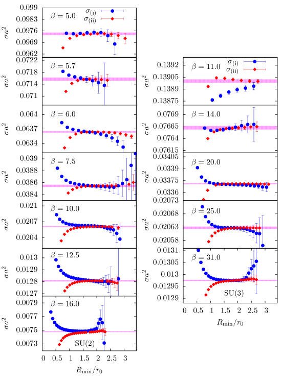
Figure 1: Results for the string tension in SU(2) (left) and SU(3) (right) gauge theory extracted from method (i), $\sigma_{\rm(i)}$, and (ii), $\sigma_{\rm(ii)}$, as explained in the text, versus the minimal value of $R$ included in the fit, $R_{\rm min}$ in units of $r_{0}$. The red bands are the values for $\sigma_{(ii)}$ which we will use for the further analysis.

The results obtained from the two methods, denoted as $\sigma_{\rm(i)}$ and $\sigma_{\rm(ii)}$, respectively, are shown in figure 1 for $\text{SU}(2)$ (left) and $\text{SU}(3)$ (right). The plots indicate that in most of the cases the extraction of $\sigma$ is reliable. The most critical case is $\beta=11.0$ for SU(3), whose value of $\sigma$ we exclude from the following analysis. Another critical case is $\beta=16.0$ for SU(2), where the two plateaus for $\sigma_{\rm(i)}$ and $\sigma_{\rm(ii)}$ do not agree within errors. In that case we use the extent where the two results are closest (the discrepancy is of order $1\sigma$). The resulting values for $\sigma$ are listed in table 3 together with the other fit parameters and are indicated by the bands in the figures. The plots indicate that within the region where the two fits agree the particular choice for $R_{\rm min}$ does not matter within the given uncertainties. In the following analysis we will use $\sigma_{\rm(ii)}$, whose value is shown as the red band in figure 1.

			(i)		(ii)
$N$	$\beta$	$r_{0}/a$	$\sqrt{\sigma}r_{0}$	$\gamma$	$\sqrt{\sigma}r_{0}$	$aV_{0}$
2	5.0	3.9472(4)( 7)	1.2325(14)(1)	0.129(16)	1.2321(5)(1)	0.2148(6)
	5.7	4.6072(4)(10)	1.2321(16)(1)	0.141(13)	1.2325(4)(1)	0.2031(4)
	6.0	4.8880(2)( 4)	1.2330( 3)(1)	0.136( 2)	1.2331(4)(1)	0.1976(1)
	7.5	6.2860(4)( 3)	1.2341( 6)(1)	0.135( 6)	1.2341(3)(1)	0.1740(2)
	10.0	8.6021(4)( 8)	1.2349( 8)(1)	0.136( 9)	1.2350(3)(1)	0.1449(2)
	12.5	10.9085(7)(16)	1.2345( 7)(1)	0.136( 6)	1.2346(3)(1)	0.1248(1)
	16.0	14.2958(6)(10)	1.2401(32)(1)	0.092(33)	1.2364(5)(1)	0.1026(2)
3	11.0	3.2881(2)( 6)	1.2256( 2)(1)	0.139( 3)	1.2259(1)(1)	0.2498(2)
	14.0	4.4433(3)( 1)	1.2303( 9)(1)	0.129( 9)	1.2300(3)(1)	0.2239(3)
	20.0	6.7075(4)( 2)	1.2318( 2)(1)	0.138( 2)	1.2318(1)(1)	0.18196(6)
	25.0	8.5797(4)( 6)	1.2322( 3)(1)	0.135( 3)	1.2322(1)(1)	0.15709(6)
	31.0	10.8182(4)( 5)	1.2323( 3)(1)	0.134( 3)	1.2323(1)(1)	0.13550(5)

Table 3: Results for the Sommer parameter $r_{0}$ and the string tension $\sigma$ in units of $r_{0}$ from methods (i) and (ii), as explained in the text. Also listed are the other fitparameters, the Lüscher constant $\gamma$ and the normalisation constant $V_{0}$.

We want to obtain the asymptotic $R\to\infty$ behaviour of the potential in the continuum. To this end we perform a continuum extrapolation for $\sqrt{\sigma}$ of the form,

$$\sqrt{\sigma}r_{0}=\big{(}\sqrt{\sigma}r_{0}\big{)}^{\rm cont}+b_{\sigma,1}\Big{(}\frac{a}{r_{0}}\Big{)}^{2}+b_{\sigma,2}\Big{(}\frac{a}{r_{0}}\Big{)}^{4}\,.$$ (21)

In practice, we perform two fits, one with $b_{\sigma,2}\neq 0$ and another one with $b_{\sigma,2}=0$. The continuum extrapolations for $\text{SU}(2)$ and $\text{SU}(3)$ are displayed in figure 2 and the results are tabulated in table 4. For the fit with $b_{\sigma,2}=0$ and SU(3) we could only include points with $(a/r_{0})^{2}<0.03$ to obtain a reasonable $\chi^{2}/$dof. We have applied a similar cut for the fit in the case of SU(2), too. For SU(2) the three results at the smallest lattice spacings show fluctuations, which for $\beta=16.0$ are bigger than $1\sigma$ with respect to the fits, leading to a $\chi^{2}/$dof$>1$. The continuum results from the two fits agree well in both cases. In the following we will use the result coming from the analysis with $b_{\sigma,2}\neq 0$.

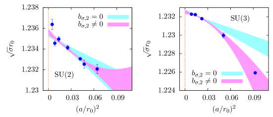
Figure 2: Continuum extrapolations of $\sqrt{\sigma_{(ii)}}r_{0}$ for SU(2) (left) and SU(3) gauge theory (right).

	SU(2)		SU(3)
	quadratic	linear	quadratic	linear
$\big{(}\sqrt{\sigma}r_{0}\big{)}^{\rm cont}$	1.2356(3)	1.2355(3)	1.2325(3)	1.2327(2)

Table 4: Results from the continuum extrapolations with $b_{\sigma}=0$ (linear) and $b_{\sigma}\neq 0$ (quadratic).

3.2 The static potential

In figure 3 we show the results for the static potential, rescaled via

$$V^{\rm RS}(R)=\Big{(}\frac{V(R)-V_{0}}{\sqrt{\sigma}}-R\sqrt{\sigma}\Big{)}\frac{R\sqrt{\sigma}}{\pi}+\frac{1}{24}\,.$$ (22)

In this rescaled form the leading order potential to $O(1/R)$ in the $1/R$ expansion is normalised to 0, so that small differences become visible. We have rescaled the energies using the string tension for each individual value of $\beta$. The solid lines in the plot correspond to the LC spectrum, eq. (7), and are evaluated using the continuum extrapolated string tension. For SU(2) gauge theory we have not plotted the potential for the two largest lattice spacings for which the results look similar.

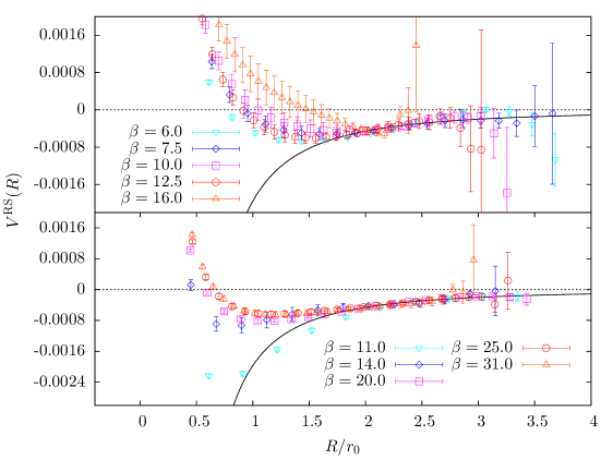
Figure 3: Results for the static potential (in its rescaled form – see eq. (22)) for different lattice spacings versus $R$ in SU(2) (top) and SU(3) (bottom) gauge theory. The black continuous line is the light cone potential from eq. (7) using the continuum extrapolated string tension.

Corrections to the LC spectrum start at around $R/r_{0}\approx 2$ (i.e. around 1 fm in 4d physical units) and are positive, except for one case, namely $\beta=11.0$ for SU(3). This means that the dominant corrections are not expected to be due to the rigidity term from section 2.3. In that case one would expect to obtain a negative correction for intermediate values of $R/r_{0}$. However, this does not rule out the presence of the rigidity term in general. It can still be a subleading correction for the lattice spacings considered. The only exception is the SU(3) $\beta=11.0$ lattice (with $a\approx 0.15$ fm – in physical units defined via $r_{0}\equiv 0.5$ fm), where the negative correction could be due to a dominant rigidity term. In all of the cases we observe that the magnitude of the corrections becomes stronger when we approach the continuum limit. In particular, they are larger for SU(2) gauge theory than for the SU(3) case.

3.3 Isolating the leading order correction terms

On top of the leading order behaviour (the LC spectrum from eq. (7)), the EST predicts corrections starting at $O(R^{-4})$. We would now like to test whether this prediction is true. The first step is to isolate the leading order correction to eq. (7). If eq. (7) is incorrect, corrections will appear with an exponent $0<m<4$, if the EST predictions are correct and $\bar{b}_{2}\neq 0$, we expect $m=4$, if corrections only appear at higher orders we will obtain $m>4$. If eq. (7) is correct to all orders we should obtain $m\approx 0$.

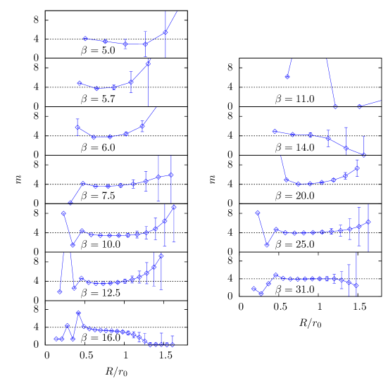
Figure 4: Results for the exponent $m$ plotted versus the minimal value of $R$ included in the fit, $R_{\rm min}$, for SU(2) (left) and SU(3) (right) gauge theory. The horizontal line indicates the LO exponent of the EST.

To investigate the power of the leading order correction we fit the data to the form

$$V(R)=E_{0}^{\rm LC}(R)+\frac{\eta}{\big{(}\sqrt{\sigma}R\big{)}^{m}}+V_{0}\,,$$ (23)

where $E_{0}^{\rm LC}(R)$ is the potential obtained from the LC energy levels (7) and $\eta$ and $m$, together with $\sigma$ and $V_{0}$, are fit parameters. The results for the exponent $m$ versus the minimal value of $R$ included in the fit, $R_{\rm min}$, is shown in figure 4. The results for the exponent typically show a plateau in the region $0.5\lesssim R/r_{0}\lesssim 1.0$ where $m\approx 4$. The only exception is, once more, $\beta=11.0$ for SU(3). For SU(2), we see that the result for $m$ is typically a bit smaller than 4 (around 3.6). This could indicate that we observe a mixing of two types of corrections where the one of $O(R^{-4})$ is the dominant one. For $R_{\rm min}/r_{0}>1$ we cannot resolve the correction terms reliably, so that $m$ is not determined sufficiently.

4 Analysis of boundary corrections without massive modes

In this section we will now turn towards the extraction of the boundary coefficient $\bar{b}_{2}$. In this first part of the analysis we will neglect contributions from massive modes (or the rigidity term) and extract the value of $\bar{b}_{2}$ in this setup. We will see how $\bar{b}_{2}$ changes in the presence of these terms in the next section.

4.1 Extraction of the boundary coefficient

To extract $\bar{b}_{2}$ we use the groundstate energy from eq. (10). To check for the impact of higher order correction terms our general fit formula is of the form

$$V(R)=E^{\rm EST}_{0}(R)+\frac{\gamma^{(1)}_{0}}{\sqrt{\sigma^{5}}R^{6}}+\frac{\gamma^{(2)}_{0}}{\sigma^{3}R^{7}}+V_{0}\,,$$ (24)

where we have included appropriate powers of $\sigma$ multiplying the higher order terms to keep the coefficients dimensionless. In practice, we perform five different types of fits:

1. we use the string tension and $V_{0}$ extracted from method (ii) in the determination of the string tension from section 3.1 and use eq. (24) with $\bar{b}_{2}$, $\gamma^{(1)}_{0}$ and $\gamma^{(2)}_{0}$ as free parameters;

2. use $\sigma$, $V_{0}$ and $\bar{b}_{2}$ as free parameters and $\gamma^{(1)}_{0}=0$ and $\gamma^{(2)}_{0}=0$;

3. use $\sigma$, $V_{0}$, $\bar{b}_{2}$ and $\gamma^{(1)}_{0}$ as free parameters and $\gamma^{(2)}_{0}=0$;

4. use $\sigma$, $V_{0}$, $\bar{b}_{2}$ and $\gamma^{(2)}_{0}$ as free parameters and $\gamma^{(1)}_{0}=0$;

5. use $\sigma$, $V_{0}$, $\gamma^{(1)}_{0}$ and $\gamma^{(2)}_{0}=0$ as free parameters and $\bar{b}_{2}=0$.

From the analysis in the previous section, we expect the correction terms to be relevant starting with $R/r_{0}\approx 1.2$. To test the region in which the data is well described by the higher order terms we perform the fits for several values of the lower cut in $R$ and check at which value for $R_{\rm min}$ we get a good description, indicated by acceptable values for $\chi^{2}/$dof. For the final result, i.e. for the $R_{\rm min}$ in the final fit, we pick the second smallest distance for which the fit gave an acceptable $\chi^{2}/$dof$<1.5$. We use the results with minimal $R$ value of $R_{\rm min}\pm 1a$ to estimate the systematic uncertainty of the extraction of the fit parameters for this particular fit. For the fits including terms of $O(R^{-6})$ or $O(R^{-7})$ we would expect that these work well down to even smaller values of $R_{\rm min}$ than the fits including only the $R^{-4}$ term, since these fits include higher order correction terms which should improve the agreement with the data.

Fit	$\sqrt{\sigma}r_{0}$	$aV_{0}$	$\bar{b}_{2}\cdot 10^{2}$	$\gamma^{(1)}_{0}\cdot 10^{3}$	$\gamma^{(2)}_{0}\cdot 10^{3}$	$\chi^{2}/$dof	$R_{\rm min}/r_{0}$
$\beta=5.0$
A	—	—	1.7(21)(23)	7(21)(75)	- 6(17)(76)	0.17	0.76
B	1.2138(2)(3)	0.2151(1)(3)	-1.75( 3)(22)	—	—	0.22	0.76
C	1.2320(3)(3)	0.2148(3)(4)	-2.29(32)(102)	-2( 2)( 7)	—	0.12	0.76
D	1.2320(3)(3)	0.2148(3)(3)	-2.15(24)(79)	—	-1.3(7)(6)	0.24	0.76
E	1.2321(3)(3)	0.2148(5)(4)	—	-67(73)(60)	-64(71)(86)	0.11	1.01
$\beta=5.7$
A	—	—	1.6( 7)(16)	60( 4)(38)	-45( 3)(31)	0.01	0.87
B	1.2329(3)(1)	0.2027(3)(1)	-1.96(21)(26)	—	—	0.03	1.09
C	1.2329(4)(2)	0.2027(4)(3)	-1.99(59)(114)	0.3(25)(80)	—	0.03	0.87
D	1.2329(4)(2)	0.2027(4)(2)	-1.98(44)(80)	—	-0.2(18)(68)	0.03	0.87
E	1.2327(3)(3)	0.2029(3)(3)	—	33(33)(12)	-24(24)(12)	0.01	0.87
$\beta=6.0$
A	—	—	2.26(61)(140)	97( 8)(47)	-80( 5)(45)	0.15	1.02
B	1.2333(1)(1)	0.1973(1)(1)	-2.19(6)(12)	—	—	0.25	1.02
C	1.2333(1)(1)	0.1973(1)(1)	-2.27(15)(60)	-1.3(6)(41)	—	0.28	0.82
D	1.2333(1)(1)	0.1973(1)(1)	-2.20(12)(39)	—	-0.9(4)(32)	0.27	0.82
E	1.2332(2)(1)	0.1975(2)(1)	—	43(44)(25)	-35(36)(35)	0.19	1.02
$\beta=7.5$
A	—	—	-0.5(14)(14)	31(18)(39)	-22(12)(35)	0.16	0.80
B	1.2342(2)(2)	0.1738(1)(1)	-2.30(7)(17)	—	—	0.05	0.95
C	1.2343(2)(1)	0.1738(2)(1)	-2.69(20)(21)	-2.3(7)(9)	—	0.03	0.80
D	1.2343(2)(1)	0.1738(1)(1)	-2.54(14)(20)	—	-1.6(5)(8)	0.03	0.80
E	1.2342(2)(2)	0.1739(2)(2)	—	52(53)(15)	-43(43)(16)	0.03	0.95
$\beta=10.0$
A	—	—	-0.95(127)(117)	28(17)(33)	-21(11)(29)	0.52	0.81
B	1.2350(1)(2)	0.14486(5)(9)	-2.42(4)(17)	—	—	0.28	0.93
C	1.2350(1)(3)	0.14482(5)(13)	-2.78(6)(36)	2.2(2)(12)	—	0.19	0.70
D	1.2350(1)(3)	0.14484(5)(14)	-2.58(5)(29)	—	-1.3(1)(10)	0.27	0.70
E	1.2349(2)(2)	0.14491(7)(10)	—	55(55)(16)	-45(45)(19)	0.17	0.93
$\beta=12.5$
A	—	—	0.53(73)(96)	47(9)(25)	-33(6)(21)	0.28	0.83
B	1.2347(1)(2)	0.12467(4)(8)	-2.27(3)(12)	—	—	0.33	0.83
C	1.2349(2)(1)	0.12458(5)(5)	-2.75(9)(18)	-2.1(3)(7)	—	0.06	0.73
D	1.2349(2)(1)	0.12460(5)(5)	-2.58(7)(16)	—	-1.3(2)(5)	0.07	0.73
E	1.2346(2)(2)	0.12476(5)(9)	—	39(39)(9)	-28(28)(9)	0.17	0.83
$\beta=16.0$
A	—	—	-0.2(8)(110)	60(9)(36)	-50(5)(33)	1.20	0.91
B	1.2357(1)(2)	0.10281(3)(5)	-2.56(3)(14)	—	—	0.95	0.91
C	1.2358(1)(3)	0.10277(3)(7)	-3.01(5)(28)	-2.6(2)(10)	—	0.76	0.70
D	1.2358(1)(2)	0.10275(3)(5)	-2.97(6)(22)	—	-2.2(2)(10)	0.54	0.77
E	1.2356(2)(2)	0.10285(4)(7)	—	55(55)(13)	-44(44)(14)	0.63	0.91

Table 5: Results of the fits for the extraction of $\bar{b}_{2}$ for $\text{SU}(2)$ gauge theory.

Fit	$\sqrt{\sigma}r_{0}$	$aV_{0}$	$\bar{b}_{2}\cdot 10^{2}$	$\gamma^{(1)}_{0}\cdot 10^{3}$	$\gamma^{(2)}_{0}\cdot 10^{3}$	$\chi^{2}/$dof	$R_{\rm min}/r_{0}$
$\beta=11.0$
A	—	—	1.6( 5)(19)	14(8)(92)	- 3(6)(100)	0.07	0.91
B	1.2259(1)(1)	0.2498(1)(2)	1.0( 2)( 9)	—	—	0.02	1.52
C	1.2260(1)(2)	0.2497(1)(4)	1.3( 2)(13)	10(6)(12)	—	0.05	0.91
D	1.2260(1)(2)	0.2497(1)(4)	0.8(10)(11)	—	8(1)( 12)	0.07	0.91
E	1.2260(1)(2)	0.2496(1)(3)	—	-17(2)(46)	22(2)( 64)	0.12	0.91
$\beta=14.0$
A	—	—	0.81(15)(43)	6(10)(11)	- 3(6)( 10)	0.05	0.68
B	1.2300(2)(1)	0.2239(1)(2)	-1.37( 4)(10)	—	—	0.02	0.90
C	1.2300(2)(2)	0.2239(2)(2)	-1.24( 9)(30)	0.7(3)( 5)	—	0.01	0.68
D	1.2300(2)(1)	0.2239(2)(1)	-1.29( 7)(10)	—	0.4(2)( 3)	0.01	0.68
E	1.2299(2)(1)	0.2240(2)(2)	—	23(5)(18)	-17(5)( 23)	0.03	0.90
$\beta=20.0$
A	—	—	-0.44(26)(63)	17(3)(18)	-11(2)( 15)	0.11	0.75
B	1.2319(2)(0)	0.18166(4)(1)	-1.71( 2)( 1)	—	—	0.003	0.89
C	1.2319(2)(0)	0.18166(5)(1)	-1.73( 6)( 8)	-0.1(2)( 2)	—	0.004	0.75
D	1.2319(2)(0)	0.18166(5)(1)	-1.72( 4)( 5)	—	-0.1(1)( 1)	0.004	0.75
E	1.2318(2)(1)	0.18178(5)(7)	—	30(2)( 8)	-22(2)( 9)	0.02	0.89
$\beta=25.0$
A	—	—	0.2( 4)(110)	41(5)(48)	-32(3)( 53)	0.04	0.93
B	1.2319(1)(0)	0.15696(3)(2)	-1.78( 2)( 4)	—	—	0.004	0.93
C	1.2319(1)(1)	0.15695(3)(10)	-1.83( 4)(32)	-0.3(2)( 5)	—	0.004	0.70
D	1.2319(1)(1)	0.15695(3)(8)	-1.81( 3)(19)	—	-0.2(1)( 5)	0.004	0.70
E	1.2318(2)(1)	0.15704(4)(7)	—	36(3)(17)	-28(3)( 23)	0.03	0.93
$\beta=31.0$
A	—	—	0.0( 4)( 6)	28(4)(15)	-19(3)( 13)	0.55	0.83
B	1.2324(1)(1)	0.13542(2)(2)	-1.77( 1)( 2)	—	—	0.34	0.74
C	1.2324(1)(2)	0.13540(2)(6)	-1.84( 2)(15)	-0.23(5)(41)	—	0.24	0.65
D	1.2324(1)(1)	0.13541(2)(5)	-1.81( 8)(10)	—	-0.12(3)( 21)	0.25	0.65
E	1.2322(1)(1)	0.13552(2)(5)	—	27(28)( 5)	-19(19)( 6)	0.46	0.83

Table 6: Results of the fits for the extraction of $\bar{b}_{2}$ for $\text{SU}(3)$ gauge theory.

The results of the fits are listed in table 5 for $\text{SU}(2)$ gauge theory and in table 6 for the $\text{SU}(3)$ case. Let us discuss the individual fits before moving on with the analysis. In general, the fits lead to small values of $\chi^{2}/$dof (since we picked the second possible value for $R_{\rm min}$), so that it is difficult to make statements about the agreement of the EST predictions with the data based on these numbers. Accordingly, our main argument to judge the agreement will be based on the values of $R_{\rm min}$ which can be used in the fits. At coarse lattice spacings all fits work equally well, leading to similar of $R_{\rm min}$. When going to smaller lattice spacings, however, the picture changes slightly. In these cases the worst fits are typically fit B (which is not surprising since higher order terms have been neglected) and fits A and E. For fit A this might be due to the fact that the fit does not allow $\sigma$ and $V_{0}$ to change, which, apparently, is to restrictive, even though both do not change significantly for the other fits. For fit E $R_{\rm min}$ needs to be larger even though higher order terms are included in the fit, indicating less agreement with the data. This implies that the scenario with $\bar{b}_{2}=0$ is disfavoured, in agreement with the analysis from section 3.3. For the following analysis we will thus include the results from fits C and D together with the one from fit B, for which the larger value of $R_{\rm min}$ has been expected. We note, however, that we cannot fully exclude the possibility that the coefficient of the $R^{-4}$ term is 0 and that the result from section 3.3 is due to a fine-tuned combination of higher order terms.

$\text{SU}(2)$		$\text{SU}(3)$
$\beta$	$\bar{b}_{2}$	$\beta$	$\bar{b}_{2}$
5.0	-0.0179( 5)(50)(23)	11.0	0.0100(15)(34)(95)
5.7	-0.0196(25)( 3)( 2)	14.0	-0.0133( 6)(10)( 2)
6.0	-0.0211( 7)(17)(11)	20.0	-0.0171( 3)( 7)( 2)
7.5	-0.0244(11)(25)(16)	25.0	-0.0175( 8)( 7)( 2)
10.0	-0.0251( 5)(27)(22)	31.0	-0.0178( 6)( 7)( 3)
12.5	-0.0245( 5)(31)(13)
16.0	-0.0273( 4)(29)(17)

Table 7: Final results for $\bar{b}_{2}$ for the individual lattice spacings. The first error is the statistical uncertainty, the second the systematic one due to the unknown correction terms, estimated by calculating the maximal deviations of the results for $\bar{b}_{2}$ from fits B to C, and the third is the systematic one associated with the choice for $R_{\rm min}$.

We determine the associated result for $\bar{b}_{2}$ on a single lattice spacing using the average over the results from fits B to D, weighted with the associated uncertainties. To determine the systematic error due to the particular choice for $R_{\rm min}$ we repeat the same procedure with $R_{\rm min}\pm 1a$ and take the maximal deviation as an estimate. The results are listed in table 7. In the next section we discuss the associated continuum extrapolation. It is interesting to note that in $\text{SU}(3)$ gauge theory the systematic errors are typically an order of magnitude smaller than in the $\text{SU}(2)$ gauge theory. A possible reason could be, that the agreement between the effective string theory predictions and the energy levels becomes better with increasing $N$. This appears natural in the light of possible corrections to the EST discussed in section 2.1, which are expected to be further suppressed with increasing $N$.

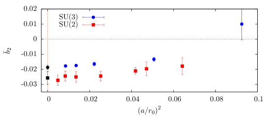
Figure 5: Results for $\bar{b}_{2}$ from table 7 versus the squared lattice spacing in units of $r_{0}$. Also shown are the continuum results from eq. (30).

The results for $\bar{b}_{2}$ are plotted versus $a^{2}$ in figure 5. The plot displays the rather smooth behaviour towards the continuum ($a=0$). The exception is the data point at $\beta=11.0$ for gauge group $\text{SU}(3)$, which shows a rather strong upwards trend. We have excluded this data point from the following analysis, since it appears to lie outside of the scaling region.

4.2 Continuum limit of boundary corrections

Up to now the comparison with the EST has been done at finite lattice spacing. To extract the final continuum results we have to perform the continuum extrapolation. To this end we parameterise the boundary coefficient $\bar{b}_{2}$ as

$$\bar{b}_{2}=\big{(}\bar{b}_{2}\big{)}^{\rm cont}+b_{\bar{b}_{2},1}\Big{(}\frac{a}{r_{0}}\Big{)}^{2}+b_{\bar{b}_{2},2}\Big{(}\frac{a}{r_{0}}\Big{)}^{4}\,.$$ (25)

Using this parameterisation we now perform three different fits:

1. a fit including all terms in eq. (25) and all lattice spacings (except for $\beta=11.0$ for $\text{SU}(3)$);

2. fit (1) but with $b_{\bar{b}_{2},2}=0$;

3. a fit with $b_{\bar{b}_{2},2}=0$, including only the $\beta$-values 7.5, 10.0, 12.5 and 16.0 for $\text{SU}(2)$ gauge theory and 20.0, 25.0 and 31.0 for $\text{SU}(3)$.

As discussed above, we have excluded the data set with $\beta=11.0$. In all cases we have included systematic errors due to the functional form and the particular value for $R_{\rm min}$ used for the extraction of $\bar{b}_{2}$ by performing these fits for the results from fits B to D and the fits with a minimal $R$ value of $R_{\rm min}\pm 1a$ individually.

To determine the final result, we have averaged the results weighted with the individual uncertainties of the extrapolations for fits B to C and estimated the systematic uncertainty due to the choice for $R_{\rm min}$ by doing the same for $R_{\rm min}\pm 1a$. The procedure is the same as the one used for the averaging at the individual lattice spacings. In this way we obtain a final result for the three different fits (1) to (3). The continuum results for $\bar{b}_{2}$ for the different fits are given in table 8. As can be seen from figure 5, the data is consistent with a straight line, which is also indicated by good values for $\chi^{2}/$dof, below but close to 1, for fit (2), even though they still might show a slight curvature. As our final result we thus use the result from fit (2), including the spread of the results from fits (1) and (3) as a systematic uncertainty associated with the continuum extrapolation. The associated curves from fit (2) with the main value for $R_{\rm min}$ are shown in figure 6.

$N$	Fit	(1)	(2)	(3)
2	$\big{(}\bar{b}_{2}\big{)}^{\rm cont}$	-0.0254(5)(42)(27)	-0.0257(3)(38)(17)	-0.0256(5)(37)(16)
3	$\big{(}\bar{b}_{2}\big{)}^{\rm cont}$	-0.0185(3)(14)(10)	-0.0187(2)(13)( 4)	-0.0186(2)(15)( 8)

Table 8: Results for $\big{(}\bar{b}_{2}\big{)}^{\rm cont}$ from fits (1) to (3) (see text). The first error is the statistical uncertainty, the second one the one associated with the unknown higher order correction terms in the potential and the third one the one due to the choice for $R_{\rm min}$.

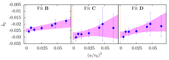
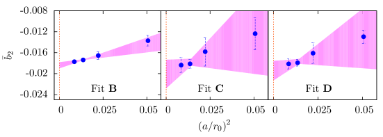
Figure 6: Results for the linear continuum extrapolation, fit (2), for the results for $\bar{b}_{2}$ obtained from fits B, C and D (from left to right) for $\text{SU}(2)$ (top) and $\text{SU}(3)$ (bottom) gauge theory.

The final continuum results for $\bar{b}_{2}$, given in eq. (30) in section 6, are already shown in figure 5. The figure indicates that the results for $\bar{b}_{2}$ in $\text{SU}(3)$ gauge theory are significantly larger than the results for $\text{SU}(2)$, indicating the non-universality of the boundary corrections in the EST. In particular, this difference remains in the continuum limit. From the tendency between $\text{SU}(2)$ and $\text{SU}(3)$, one might think that $\bar{b}_{2}$ tends to zero for $N\to\infty$. This will be investigated further in the next publication of the series.

5 Analysis of boundary corrections with massive modes

Up to now we have ignored possible contributions from massive modes. Our aim in this section is to see how the presence of these modes changes the result for $\bar{b}_{2}$ from the previous section.

5.1 Testing the consistency with the potential

To include the massive modes in the analysis we include the terms from eqs. (13) and (14) in the fit function eq. (24),

$$V(R)=E_{0}^{\rm eff}(R)-\frac{m}{2\pi}\sum_{k=1}^{\infty}\frac{K_{1}(2kmR)}{k}-\frac{(d-2)(d-10)\pi^{2}}{3840m\sigma R^{4}}+\frac{\gamma^{(1)}_{0}}{\sqrt{\sigma^{5}}R^{6}}+\frac{\gamma^{(2)}_{0}}{\sigma^{3}R^{7}}+V_{0}\,.$$ (26)

The main difficulty when fitting to eq. (26) is the presence of the infinite sum over the modified Bessel functions of the second kind. In practice, however, the sum is always completely dominated by the first few terms, since $K_{1}(nc)$ decays exponentially with increasing $n$ for any positive real number $c$. In our fits we have used the first 100 terms and checked explicitly the correction to this approximation by calculating the corrections due to the next 10 terms in the sum. For all combinations of $m$ and $R$ that appeared in our analysis the correction has been suppressed by 100 orders of magnitude, at least.

Using eq. (26) we have performed the four different types of fits:

1. use $\sigma$, $V_{0}$, $\bar{b}_{2}$ and $m$ as free parameters and $\gamma^{(1)}_{0}=\gamma^{(2)}_{0}=0$;

2. use $\sigma$, $V_{0}$, $\bar{b}_{2}$, $m$ and $\gamma^{(1)}_{0}$ as free parameters and $\gamma^{(2)}_{0}=0$;

3. use $\sigma$, $V_{0}$, $\bar{b}_{2}$, $m$ and $\gamma^{(2)}_{0}$ as free parameters and $\gamma^{(1)}_{0}=0$;

4. use $\sigma$, $V_{0}$ and $m$ as free parameters and $\gamma^{(1)}_{0}=\gamma^{(2)}_{0}=\bar{b}_{2}=0$;

The last fit constitutes a check whether the presence of the $R^{-4}$ term due to the massive mode (i.e. the term from eq. (14)) is already sufficient to describe the $R^{-4}$ correction found in section 3.3.

Fit	$\sqrt{\sigma}r_{0}$	$aV_{0}$	$\bar{b}_{2}\cdot 10^{2}$	$r_{0}m$	$\gamma^{(1)/(2)}_{0}\cdot 10^{3}$	$\chi^{2}/$dof	$R_{\rm min}/r_{0}$
$\beta=5.0$
F	1.2320(2)(1)	0.2148(2)(2)	-0.8( 1)( 4)	2.75( 6)(49)	—	0.12	0.76
G	1.2322(4)(2)	0.2145(5)(3)	-2.0( 3)( 1)	2.01(70)(45)	-6.3(12)(56)	0.11	0.76
H	1.2322(3)(2)	0.2145(4)(3)	-1.7(11)( 8)	2.06(44)(50)	-3.6(52)(35)	0.10	0.76
J	1.2320(3)(2)	0.2149(3)(3)	—	2.63( 7)(22)	—	0.19	1.52
$\beta=5.7$
F	1.2331(10)(2)	0.2024(12)(3)	-1.3( 8)( 6)	2.1(149)(607)	—	0.06	0.87
G	1.2328(8)(5)	0.2026(10)(7)	-7.4(321)(73)	1.2(150)(40)	-45(220)(81)	0.02	0.87
H	1.2329(5)(3)	0.2027(7)(3)	-1.2(17)( 7)	5.5(69)(24)	-0.8(71)(19)	0.03	0.87
J	1.2327(2)(4)	0.2029(2)(4)	—	2.93(19)(89)	—	0.06	1.30
$\beta=6.0$
F	1.2333(1)(1)	0.1973(1)(1)	-1.0( 1)(10)	3.5( 5)(238)	—	0.29	0.82
G	1.2333(2)(2)	0.1972(1)(3)	-6.7( 6)(69)	1.3( 1)(27)	-37(42)(710)	0.33	0.82
H	1.2333(2)(2)	0.1972(2)(3)	-4.9( 5)(52)	1.4( 1)(25)	-21( 3)(57)	0.34	0.82
J	1.2332(1)(2)	0.1975(1)(2)	—	2.88(33)(454)	—	0.27	1.43
$\beta=7.5$
F	1.2343(2)(3)	0.1738(1)(2)	-1.15( 5)(14)	2.9( 2)( 6)	—	0.08	0.80
G	1.2345(3)(2)	0.1736(4)(2)	-5.1(63)(38)	1.5(37)(18)	-24(37)(30)	0.06	0.80
H	1.2345(5)(2)	0.1736(5)(3)	-3.7(53)(26)	1.6(68)(15)	-12(25)(22)	0.06	0.80
J	1.2341(2)(2)	0.1740(1)(2)	—	2.70( 8)(15)	—	0.11	1.43
$\beta=10.0$
F	1.2351(1)(2)	0.14475(6)(8)	-1.47(11)(18)	2.6( 2)( 3)	—	0.10	0.93
G	1.2352(2)(2)	0.14472(2)(2)	-1.74(42)(23)	2.7( 6)(10)	-3( 2)(13)	0.06	0.70
H	1.2352(2)(2)	0.1447 (2)(2)	-1.67(33)(29)	2.6( 4)( 3)	-2( 2)( 2)	0.07	0.70
J	1.2348(1)(2)	0.14497(5)(9)	—	2.75( 3)(11)	—	0.50	1.40
$\beta=12.5$
F	1.2349(2)(2)	0.12459(5)(6)	-1.27( 5)( 9)	3.0( 3)( 4)	—	0.11	0.83
G	1.2349(2)(2)	0.12456(7)(5)	-1.49(11)(13)	3.2( 4)( 3)	-2.0( 6)( 8)	0.08	0.64
H	1.2349(2)(2)	0.12456(7)(8)	-1.40(11)(16)	3.0( 4)( 1)	-1.2( 4)( 7)	0.09	0.64
J	1.2345(2)(2)	0.12478(4)(7)	—	2.88( 3)( 9)	—	0.42	1.28
$\beta=16.0$
F	1.2359(1)(2)	0.10273(3)(5)	-1.62( 4)(18)	2.7( 1)( 2)	—	0.60	0.91
G	1.2361(1)(2)	0.10265(3)(7)	-2.34( 9)(49)	2.4( 1)( 3)	-6.0( 5)(28)	0.35	0.70
H	1.2360(1)(2)	0.10269(3)(7)	-1.93( 6)(35)	2.5( 1)( 3)	-3.0( 2)(17)	0.47	0.70
J	1.2356(2)(2)	0.10285(4)(4)	—	2.74( 1)( 6)	—	0.88	1.40

Table 9: Results of the fits for the extraction of $\bar{b}_{2}$ and $m$ for $\text{SU}(2)$ gauge theory.

Fit	$\sqrt{\sigma}r_{0}$	$aV_{0}$	$\bar{b}_{2}\cdot 10^{2}$	$r_{0}m$	$\gamma^{(1)/(2)}_{0}\cdot 10^{3}$	$\chi^{2}/$dof	$R_{\rm min}/r_{0}$
$\beta=11.0$
F	1.2261(1)(3)	0.2493(1)(5)	-1.11( 3)(15)	1.46( 2)(32)	—	0.20	0.91
G	1.2260(1)(1)	0.2495(2)(2)	-6.2 ( 4)(62)	1.11( 3)(25)	-44( 4)(82)	0.01	0.91
H	1.2260(1)(1)	0.2495(2)(2)	-4.6 ( 3)(47)	1.15( 3)(24)	-30( 3)(76)	0.01	0.91
J	1.2260(1)(2)	0.2495(1)(3)	—	1.51( 3)(19)	—	0.05	1.52
$\beta=14.0$
F	1.2302(2)(3)	0.2236(1)(5)	-0.64( 1)(43)	2.25( 6)(37)	—	0.09	0.68
G	1.2302(2)(2)	0.2236(2)(3)	-2.5 ( 5)(25)	1.63(12)(162)	-10( 3)(13)	0.004	0.68
H	1.2302(2)(1)	0.2236(2)(1)	-1.8 ( 3)(14)	1.70(12)(71)	-5( 2)( 7)	0.005	0.68
J	1.2300(2)(1)	0.2239(1)(1)	—	2.65(35)(37)	—	0.01	1.35
$\beta=20.0$
F	1.2321(2)(1)	0.18151(4)(1)	-0.89( 2)(42)	2.36( 5)(45)	—	0.12	0.75
G	1.2321(3)(2)	0.1846 (4)(3)	-3.5 (46)(29)	1.6 (59)(29)	-15(26)(17)	0.03	0.75
H	1.2321(2)(2)	0.1815 (1)(2)	-2.5 ( 2)(12)	1.6 ( 1)(156)	-7( 1)( 8)	0.03	0.75
J	1.2318(2)(2)	0.1818 (1)(2)	—	2.93( 2)(17)	—	0.21	1.19
$\beta=25.0$
F	1.2324(1)(2)	0.1570(1)(2)	-0.92( 4)(15)	5.0 ( 4)(28)	—	0.03	0.70
G	1.2326(1)(3)	0.1568(1)(2)	-2.8 ( 2)(15)	1.7 ( 4)(272)	-10( 1)(10)	0.17	0.70
H	1.2325(1)(3)	0.1568(1)(2)	-2.0 ( 1)(12)	1.8(4)(214276)	-5( 1)( 5)	0.16	0.70
J	1.2323(1)(1)	0.1571(1)(1)	—	2.85( 4)(12)	—	0.22	1.28
$\beta=31.0$
F	1.2326(1)(1)	0.13530(2)(1)	-0.90( 1)(20)	2.55( 1)(37)	—	0.50	0.74
G	1.2327(1)(1)	0.13525(3)(1)	-3.0 ( 2)(11)	1.67( 5)(25)	-11( 1)( 7)	0.31	0.74
H	1.2327(3)(4)	0.13527(2)(2)	-2.2 ( 7)( 6)	2(335)(34)	5( 7)( 6)	0.32	0.74
J	1.2324(1)(1)	0.13543(3)(1)	—	2.57( 6)( 9)	—	0.38	1.57

Table 10: Results of the fits for the extraction of $\bar{b}_{2}$ and $m$ for $\text{SU}(3)$ gauge theory.

The fit results are tabulated in tables 9 and 10. The first thing we note is that fit J needs a value of $R_{\rm min}$ which is a factor between 1.5 and 2 larger than $R_{\rm min}$ for the other fits. In particular, $R_{\rm min}$ is typically larger than those values of $R$ where we found the $R^{-4}$ correction term to be dominant in section 3.3. This basically rules out the possibility that the boundary term is absent, in which case the full $R^{-4}$ correction would be given by the correction term from the massive modes. For the other fits the values of $R_{\rm min}$ are comparable, but typically a bit smaller than those of the fits in the previous section. This is not surprising given the fact that each fit has an additional free parameter compared to fits B to D from the previous section. When looking at the result for $\bar{b}_{2}$ and $m$ we see that the fits F to H always agree within uncertainties, since the uncertainties of the fits G and H are large. The large uncertainties are most likely due to the fact that the available data does not allow to constrain the additional fit parameter in these fits compared to fit F. In the following analysis we will thus only use the results from fit F. The uncertainties of the parameters from the other fits do not allow for any conclusions about the values of the parameters and continuum extrapolations. In this case our results for the individual lattice spacings are given by the values for fit F in tables 9 and 10 and they only have two uncertainties, namely the statistical one and the systematic uncertainty associated with the particular choice for $R_{\rm min}$ (estimated in the usual way). Unfortunately we cannot investigate the systematic uncertainty due to unknown higher order correction terms, but we believe that the presence of these terms is only a minor effect if massive modes are present.

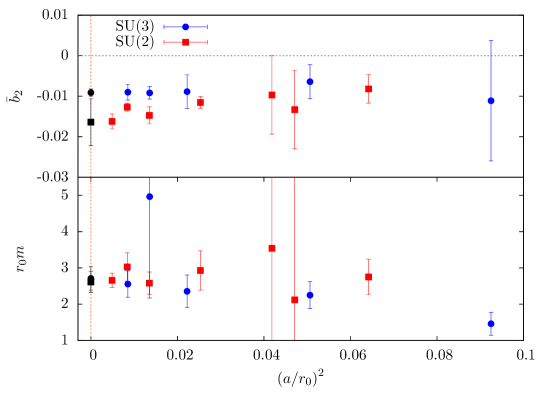
Figure 7: Results for $\bar{b}_{2}$ and $r_{0}m$ versus the squared lattice spacing in units of $r_{0}$. Also shown are the continuum results from eqs. (31) and (32).

The results for $\bar{b}_{2}$ and $r_{0}m$ are plotted versus $a^{2}$ in figure 7. In comparison to the results for $\bar{b}_{2}$ from the previous section (figure 5), the results for $\text{SU}(2)$ show stronger fluctuations in the approach to the continuum while the results for $\text{SU}(3)$ obtain larger uncertainties. In general, the results for $\bar{b}_{2}$ are closer to zero when massive modes are included. The reason for this is obviously given by the presence of the additional $R^{-4}$ term in eq. (26). This term contaminates the boundary correction term and thus reduces the magnitude of $\bar{b}_{2}$. The results for $r_{0}m$ show a rather smooth approach to the continuum with the exception of the point at $\beta=25.0$ for $\text{SU}(3)$ gauge theory, which, however, also has a large uncertainty.

5.2 Continuum extrapolations

Ultimately we are interested in the comparison between the two sets of results in the continuum. To this end we perform a continuum extrapolation similarly to the one in section 4.2 by using fits of the type (1) to (3) for $\bar{b}_{2}$ with the ansatz from eq. (25). For $r_{0}m$ the ansatz reads

$$r_{0}m=\big{(}r_{0}m\big{)}^{\rm cont}+b_{m,1}\Big{(}\frac{a}{r_{0}}\Big{)}^{2}+b_{m,2}\Big{(}\frac{a}{r_{0}}\Big{)}^{4}$$ (27)

and we perform fits of the types (1) to (3) where $b_{\bar{b}_{2},2}$ is replaced by $b_{m,2}$ in the fit definitions. The difference to section 4.2 is, that we only perform continuum extrapolations for fit F, so that no averaging in the continuum limit is necessary. Once more the fits have also been done for the results from $R_{\rm min}\pm 1a$ to assess the uncertainty associated with the choice for $R_{\rm min}$.

$N$	Fit	(1)	(2)	(3)
2	$\big{(}\bar{b}_{2}\big{)}^{\rm cont}$	-0.0164(4)(56)	-0.0151(3)(27)	-0.0164(5)(56)
3	$\big{(}\bar{b}_{2}\big{)}^{\rm cont}$	-0.0087(3)( 3)	-0.0098(1)(13)	-0.0091(2)( 5)
2	$\big{(}r_{0}m\big{)}^{\rm cont}$	2.56( 7)(31)	2.65( 3)(29)	2.61( 6)(28)
3	$\big{(}r_{0}m\big{)}^{\rm cont}$	2.75(12)(25)	2.60( 5)(62)	2.71( 9)(29)

Table 11: Results for $\big{(}\bar{b}_{2}\big{)}^{\rm cont}$ and $\big{(}r_{0}m\big{)}^{\rm cont}$ from fits (1) to (3) (see text). The first error is the statistical uncertainty, the second the systematical error due to the choice for $R_{\rm min}$.

The results for the continuum extrapolations with fits (1) to (3) are given in table 11. We usually obtain a rather good continuum extrapolation, even though for $\bar{b}_{2}$ in $\text{SU}(2)$ gauge theory the extrapolation leads to rather large values of $\chi^{2}$/dof around 5 to 10, due to the fluctuations of $\bar{b}_{2}$ for the small values of $a$. Since the continuum extrapolation is a bit more problematic in this case we will use the results from fit (3) for our final results. This fit appears to be a bit more stable than the continuum extrapolation linear in $a^{2}$ using all data points. Once more the uncertainty concerning the continuum extrapolation is estimated via the maximal difference of the result of fit (3) with respect to the result of the other fits. The continuum results for $\bar{b}_{2}$ and $r_{0}m$, given in eqs. (31) and (32) in section 6, are shown in figure 7. Owing to the figure, we expect the hierarchy between the results from $\text{SU}(2)$ and $\text{SU}(3)$ gauge theory to remain in the analysis with massive modes. The inclusion of massive modes only changes the quantitative results while retaining the qualitative features. The results for $r_{0}m$ in the continuum agree within error bars between $\text{SU}(2)$ and $\text{SU}(3)$.

6 Summary and discussion of the final results

The previous three sections contained a number of interesting results, which are, however, difficult to extract from the somewhat lengthy discussion. Before we move on to the conclusions let us thus summarise and discuss the main findings in some more detail.

6.1 Summary of results

In section 3 we have extracted the Sommer parameter and the string tension with high accuracy from our results for the static potential. The results are given in table 3. After that we have performed a continuum extrapolation of the string tension to obtain the final result

$$\big{(}\sqrt{\sigma}r_{0}\big{)}^{\rm cont}=\left\{\begin{array}[]{ll}1.2356(3)(1)&\quad\text{for}\>\>\text{SU}(2)\vspace*{2mm}\\ 1.2325(3)(2)&\quad\text{for}\>\>\text{SU}(3)\,.\end{array}\right.$$ (28)

Here the string tension has been extracted by parameterising the potential with the LC spectrum, eq. (7), up to the point where the result for $\sigma$ did agree with the NLO expansion of eq. (7). The first uncertainty is the statistical one and the second uncertainty originates from the continuum extrapolation. In three dimensions any comparison to physical units is meaningless. Nonetheless, identifying $r_{0}$ with 0.5 fm Sommer:1993ce (to define the unit ‘fm’ in three dimensions) and using the standard conversion factor $\hbar c=197.3(\ldots)$ fm MeV we obtain

$$\big{(}\sqrt{\sigma}\big{)}^{\rm cont}=\left\{\begin{array}[]{ll}487.6(2)(1)\>\>\text{MeV}&\quad\text{for}\>\>\text{SU}(2)\vspace*{2mm}\\ 486.4(2)(1)\>\>\text{MeV}&\quad\text{for}\>\>\text{SU}(3)\,,\end{array}\right.$$ (29)

respectively. A comparison to the latest results for the continuum string tension in three dimensions Lucini:2002wg ; Bringoltz:2006gp is only possible in terms of the Karabili-Kim-Nair prediction Karabali:1998yq , i.e. in terms of the continuum extrapolated coupling. We leave this type of comparison to the next publication. Our results at finite lattice spacing are fully in agreement, but more precise, than the values given in Teper:1998te ; HariDass:2007tx . With a constant continuum extrapolation the $\text{SU}(2)$ results from HariDass:2007tx give a continuum result around 1.234, which is a bit smaller but comparable to our result.

After the extraction of the leading order (linear) behaviour we have compared the results for the potential to the leading order EST prediction, namely the LC spectrum, and extracted the exponent of the leading order correction in $1/R$. The results, shown in figure 4 are consistent with an exponent of 4, as expected from the EST, where the leading order correction is the boundary term proportional to $\bar{b}_{2}$. We then extracted the value for $\bar{b}_{2}$, excluding contributions from possible massive modes (cf. section 2.3). The results at finite lattice spacing are given in table 7 and the continuum results from the individual extrapolations in table 8. As the final continuum estimates for $\bar{b}_{2}$ we obtain

$$\big{(}\bar{b}_{2}\big{)}^{\rm cont}=\left\{\begin{array}[]{ll}-0.0257\,(3)(38)(17)(3)&\quad\text{for}\>\>\text{SU}(2)\vspace*{2mm}\\ -0.0187\,(2)(13)(\>\>4)(2)&\quad\text{for}\>\>\text{SU}(3)\,.\end{array}\right.$$ (30)

The first error is purely statistical, the second is the systematical error due to the unknown correction terms to the potential, the third is the one associated with the particular choice for the minimal value of $R$ included in the fit for the extraction of $\bar{b}_{2}$, $R_{\rm min}$, and the fourth systematic uncertainty is the one due to the continuum extrapolation (for details see section 4). These values indicate that the magnitude of $\bar{b}_{2}$ decreases with increasing $N$, meaning that it could potentially vanish in the limit $N\to\infty$. The result also shows that $\bar{b}_{2}$, indeed, is non-universal, as expected since its value is not constrained in the EST.

Concerning the extraction of $\bar{b}_{2}$ the main uncertainty comes from the fact that massive modes, or, equivalently, a possible rigidity term in the EST, lead to a contaminating additional $R^{-4}$ correction. The presence of this term is expected to change the value of $\bar{b}_{2}$. At present it is unclear whether such a contamination will ultimately be present or not, so that we have to take this possibility into account. On the basis of our simulations we also cannot exclude this possibility, since the fits to the potential reported in section 5.1 work equally well compared to the results from section 4.1. We can exclude, however, the possibility that the $R^{-4}$ correction is fully due to the correction associated with the massive modes, since fit J (see section 5.1) leads to a much larger value for $R_{\rm min}$ than the other fits. Repeating the whole analysis, we see that the accuracy is only sufficient for fit F from tables 9 and 10. Using these results we obtain the continuum results listed in table 11 and the final continuum results

$$\big{(}\bar{b}_{2}\big{)}^{\rm cont}=\left\{\begin{array}[]{ll}-0.0164\,(5)(56)(13)&\quad\text{for}\>\>\text{SU}(2)\vspace*{2mm}\\ -0.0091\,(2)(\>\>5)(\>\>7)&\quad\text{for}\>\>\text{SU}(3)\,.\end{array}\right.$$ (31)

Here the first error is purely statistical, the second is the one associated with the particular choice for $R_{\rm min}$ and the third systematic uncertainty is the one due to the continuum extrapolation. In this analysis we have only been able to use one of the fits for a reliable extraction of $\bar{b}_{2}$ (fit F from tables 9 and 10), which is why one of the systematic uncertainties cannot be estimated. The comparison of eqs. (30) and (31) reveals that the inclusion of the contamination reduces the magnitude of $\bar{b}_{2}$ but does not alter the qualitative feature of a decrease in magnitude of $\bar{b}_{2}$ with increasing $N$.

From the extraction of $\bar{b}_{2}$ when massive modes are included we also obtain an estimate for the mass of the massive modes. The continuum results are listed in table 11, and as our final continuum results we get

$$\big{(}r_{0}m\big{)}^{\rm cont}=\left\{\begin{array}[]{ll}2.61\,(6)(28)(\>\>5)&\quad\text{for}\>\>\text{SU}(2)\vspace*{2mm}\\ 2.71\,(9)(29)(11)&\quad\text{for}\>\>\text{SU}(3)\,,\end{array}\right.$$ (32)

where the uncertainties are as in eq. (31). The interpretation of this “mass” is an open question. The first possibility is that it represents a massive mode on the string worldsheet, which could indicate that we observe the three-dimensional analogue to the worldsheet axion (cf. section 2.3). Recall, that the topological coupling term does not exist in 3d, so that the massive mode will appear as a quasi-free mode on the worldsheet up to coupling terms including two massive boson fields. On the other hand, the contribution could also be due to the rigidity term, in which case the results from eq. (32) can be translated into results for the coupling $\alpha$ via eq. (12). It is intriguing to note that the results for $m$, dividing by $\sqrt{\sigma}$ from eq. (28), are very similar to the results for the mass of the worldsheet axion from Dubovsky:2013gi ; Athenodorou:2017cmw , at least for the case of $\text{SU}(2)$ gauge theory. For $\text{SU}(3)$ gauge theory our result is somewhat larger than the result from Dubovsky:2013gi ; Athenodorou:2017cmw , however, in contrast to those results our result is extrapolated to the continuum. In fact, our results around $\beta=25.0$ are already fully compatible with the results from Dubovsky:2013gi ; Athenodorou:2017cmw . This opens up the possibility that, indeed, we are looking at a massive mode on the three dimensional worldsheet which is similar in nature to the worldsheet axion.

It is also important to ask whether the value for $m$ extracted in our analysis does still comply with the framework of the EST. From eq. (6) we expect modes of masses down to a few times $\sqrt{\sigma}$ to be integrated out. The masses we have obtained here are around twice as large as $\sqrt{\sigma}$. In our fits we could typically go down to $R/r_{0}\approx 0.7$. When we assume that this is a sign for the scale where the EST is bound to break down, this leads to a cut-off scale of $1.2\times\sqrt{\sigma}$. However, this estimate could well underestimate the true cut-off scale, so that a mass of $2\times\sqrt{\sigma}$ can potentially be below that bound.

6.2 Comparison between continuum EST and data

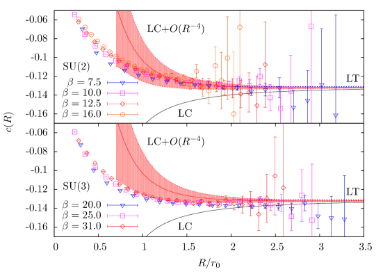
Figure 8: Results for the curvature $c(R)$ plotted versus $R/r_{0}$. The curve labeled with ‘LT’ is the Lüscher constant, the one labeled with ‘LC’ is the light cone potential with the continuum extrapolated string tension and the curve labeled with ‘LC$+O(R^{-4})$’ is the LC curve including the boundary term with the continuum extrapolated value of $\bar{b}_{2}$.

We will now compare the continuum predictions for the potential from the EST to the results for the potential on our finest lattice spacings. A suitable quantity to visualise the subleading contributions to the potential is the curvature, associated with the second derivative

$$c(R)=\frac{R^{3}}{2}\frac{\partial^{2}V(R)}{\partial R^{2}}\,.$$ (33)

In the $R\to\infty$ limit $c(r)$ is expected to reproduce the Lüscher constant $-\pi/24$. The results for $c(R)$ are compared to the continuum results for the EST in figure 8. The black curve in the figure is the LC spectrum, eq. (7), with the continuum string tensions from eq. (28) (the uncertainties are smaller than the line), and the red band includes the boundary term from eq. (10) with the continuum boundary coefficient $\bar{b}_{2}$ from eq. (30). The inclusion of the boundary term obviously enhances the agreement with the data significantly down to small values of $R$. We also note that the two curves are basically indistinguishable at the scale of the plot (they are not identical, however). For $\text{SU}(2)$ gauge theory the data at finite lattice spacing already agrees rather well with the continuum EST, while for $\text{SU}(3)$ gauge theory the data lies below the curve. We have not shown the curve including massive modes in the plot since it overlaps with the ‘LC$+O(R^{-4})$’ curve and compares very similarly to the data.

7 Conclusions

In this article we have performed a high precision study of the static $q\bar{q}$ potential in three-dimensional $\text{SU}(N)$ gauge theory with $N=2$ and 3 and compared the results to the potential obtained from the effective string theory. In particular, we obtained accurate results with full control over the systematic effects for the continuum string tension, the non-universal boundary coefficient $\bar{b}_{2}$ and, for the extended analysis, the “mass” of the possible massive mode within the EST. The results are summarised and discussed in detail in section 6.1. In particular, we could show that the leading order correction to the light cone spectrum is of $O(R^{-4})$ (cf. section 3.3). If massive modes are present, the results for $\bar{b}_{2}$ change (see eqs. (30) and (31)) due to another correction of $O(R^{-4})$, contaminating the result for $\bar{b}_{2}$. However, the contribution from the massive modes only is not enough to describe the data, so that we can conclude that $\bar{b}_{2}\neq 0$. 

The data for $\bar{b}_{2}$ shows an interesting trend towards zero with increasing $N$, leading to the possibility that $\bar{b}_{2}$ could vanish in the limit $N\to\infty$. This result is also independent of whether or not we include massive modes in the analysis. In the context of generalisations of the AdS/CFT correspondence to large $N$ gauge theories, this is an interesting result since it imposes constraints on the fundamental string theory for the dual version of Yang-Mills theories at large $N$. We will investigate this issue further in the next publication in this series of papers.

The main obstacle of our analysis for $\bar{b}_{2}$ is the fact, that it is impossible to judge whether or not massive modes, or, equivalently, the rigidity term (or even both) are present. While some properties (like the decrease in magnitude for $N\to\infty$) are independent of this issue, the exact value of $\bar{b}_{2}$ can only be extracted once the issue is resolved. To this end it would be desirable to have an expression for the excited state energies in the presence of a massive mode, or, alternatively, the rigidity term. This could potentially help to discriminate between the existence or non-existence of such terms and, in addition, it could help to discriminate between the two types of additional contributions.

It is intriguing to see that the results for the mass of the possible massive modes is in good agreement with the masses found in  Dubovsky:2013gi ; Athenodorou:2017cmw . It is thus possible that we are seeing a massive mode on the worldsheet which is similar in nature to the worldsheet axion. Note, that in 3d the topological coupling term is absent, so that the analogue to the worldsheet axion appears as a quasi-free mode on the worldsheet coupling to the GBs via the covariant derivative and possible higher order coupling terms. It will be interesting to see whether the mass of the massive modes remains consistent with the one of the worldsheet axion for $N\to\infty$.

Appendix A Simulation setup

This appendix contains the details of the numerical simulations. For the configuration updates we have used the, Cabbibo-Marinari heatbath algorithm Cabibbo:1982zn for $\text{SU}(N)$ gauge theories with all $\text{SU}(2)$ subgroups, in combination with the improved $\text{SU}(2)$ heatbath algorithm from Kennedy:1985nu . For each update we perform three overrelaxation steps Creutz:1987xi .

To obtain a clean result for the groundstate potential in terms of contaminations from excited states the spatial correlation function of two Polyakov loops is the most promising observable. Its spectral representation is given by

$$\left\langle P^{\ast}(R)\>P(0)\right\rangle=\sum_{i=0}^{\infty}b_{i}\>e^{-E_{i}(R)\>T}$$ (34)

for $R<L/2$, where $T=a\;N_{t}$ and $L=a\;N_{s}$ are the temporal and spatial lengths of the lattice, $b_{i}$ is the overlap between the operator and the associated energy eigenstate and $E_{i}(R)$ is the $i$’th energy level. We always take energies to be ordered in ascending order, i.e. $E_{0}<E_{1}<E_{2}<\ldots\;$. In the limit of $T\to\infty$ the leading contribution to eq. (34) is given by the groundstate $E_{0}(R)=V(R)$ and excited states are suppressed with $\exp\{-[E_{i}(R)-E_{0}(R)]\;T\}$. For large values of $T$ excited states can thus be neglected to a good approximation and we check in appendix B whether this is true for the temporal extents used in the present study. If we can neglect contaminations from excited states we can extract $V(R)$ via

$$V(R)=-\frac{1}{T}\ln\left[\left\langle P^{\ast}(R)\>P(0)\right\rangle\right]\;.$$ (35)

Note, that the potential is determined from the effective string theory up to a constant, which we denote as $V_{0}$ (it can also be related to the constant term $\mu$ in the boundary action (3); here, however, we are not really interested in this quantity).

The string tension can either be extracted from a fit to the potential, or via the force

$$F(R)\equiv\frac{\partial\;V(R)}{\partial R}\;,$$ (36)

given in the $1/R$ expansion of the EST in three dimensions by

$$F(R)=\sigma+\frac{\pi}{24}\;\frac{1}{R^{2}}+O(R^{-4})\,.$$ (37)

Note, that the determination via the force does not demand the determination of $V_{0}$. Here we will use both methods to extract the string tension and compare the results.

The string tension can also be used to fix the lattice spacing in physical units and observables can then be expressed in units of $a\sqrt{\sigma}$. However, the determination of $a\sqrt{\sigma}$ demands to control the asymptotic $R\to\infty$ behaviour. A more suitable observable to set the reference scale is the Sommer parameter $r_{0}$ Sommer:1993ce , which is defined implicitly by

$$r_{0}^{2}\;F(r_{0})=1.65\;.$$ (38)

$r_{0}$ can be obtained directly by interpolation of the results for $R^{2}\;F(R)$.

The reliable extraction of the potential demands the control of the contaminations from excited states and thus large temporal extents. Since the signal-to-noise ratio of such Polyakov loop correlation functions decays exponentially with $T$, the reliable extraction of the expectation values demands the use of a suitable error reduction algorithm. Our choice is to use the multilevel algorithm introduced by Lüscher and Weisz Luscher:2001up . In particular, we use one level of averaging for all lattices and the parameters such as the number of sublattice updates, $n_{t}$, and the temporal extent of the sublattices, $t_{s}$, are given in table 2.

Appendix B Control of systematic uncertainties

For the measurements of the potential there are several systematic effects that need to be controlled for a reliable extraction of the potential at a given lattice spacing. In particular, this concerns the contaminations from excited states and finite size effects. Checks concerning these two effects are reported in the following. There is yet another effect at very fine lattice spacings, owing to the “freezing” of the topological charge in certain sectors. We control this effect by using a completely new run (including full thermalisation starting from a random configuration) for at least each two measurements. This can be done since the thermalisation (we take a very conservatively long thermalisation with at least 1000 update steps) needs relatively little time compared to one measurement with the multilevel algorithm.

Excited state contributions

Following the spectral representation (34) for the Polyakov loop correlation function, the correction to eq. (35) owing to excited states is given by (see also Luscher:2002qv )

$$V(R)=-\frac{1}{T}\ln\left[\left\langle P^{\ast}(R)\>P(0)\right\rangle+w_{1}e^{-\Delta E\,T}+\ldots\right]\;.$$ (39)

The contamination from the second term on the right hand side can be checked by performing simulations for two different temporal extents $T$ of the lattice. Here we have done simulations for $\text{SU}(3)$ with $\beta=14.0$ on 48 and $64\times 48^{2}$ lattices and compare the results for the potential. The results for the difference of the two energies are shown in figure 9. As can be seen from the plot, the two sets of energies agree perfectly within errors for the whole range of $q\bar{q}$ separations considered, meaning that excited states are negligible. Since for the different ensembles $T$ changes only little in physical units, we expect this to hold for all lattices considered. Note, that the energy levels (and the overlaps) of the flux tube, in general, change only on the subleading level for different values of $N$. Consequently, we would expect this result to be valid for different values of $N$ as well.

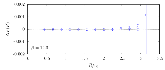
Figure 9: Difference in the results for the static potential $\Delta V$ from temporal extents 48 and 64 at $\beta=14.0$ versus the $q\bar{q}$-separation in units of $r_{0}$.

Finite size effects

For Polyakov loop correlators there are two types of finite size effects that can occur: (a) the flux tube feels the extent of the finite lattice volume perpendicular to its extension; (b) the contribution to the energies of the flux tube winding “around the world”. Relevant for effect (a) is the bulk correlation length and, with our lattice volumes, this effect should be suppressed by many orders of magnitude. Effect (b) might cause trouble and its effect should be investigated. Including the winding contribution, the Polyakov loop correlator is to leading order given by

$$\left\langle P^{\ast}(R)\>P(0)\right\rangle=b_{0}\>\left[e^{-E_{0}(R)\>T}+e^{-E_{0}(L-R)\>T}\right]\,.$$ (40)

Since $E_{0}(R)$ growths linearly with $R$, we expect the winding contribution to be strongly suppressed when $L-R>R$.

Assuming the leading order linear relation $\sigma R$ for the bare energy in lattice units and a relative error of $10^{-3}$ for the Polyakov loop correlator (which is a lower bound for what we get for the larger $R$ values), we see that the second term is negligible if

$$\frac{1}{2}\Big{(}\sqrt{\sigma}L-\frac{\ln(3)}{\sqrt{\sigma}T}\Big{)}>\sqrt{\sigma}R\quad\Rightarrow\quad\sqrt{\sigma}R<6.1\,,$$ (41)

where in the second step we have used that for our lattices $T=L$ and $\sqrt{\sigma}L\gtrsim 12.3$. This condition is always fulfilled in our study.

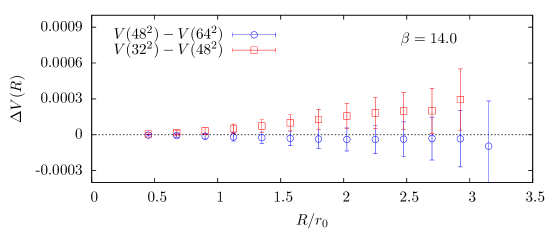
Figure 10: Difference in the results for the static potential $\Delta V$ from volumes $48^{2}$ and $64^{2}$ (blue circles) and $32^{2}$ and $48^{2}$ with $N_{t}=48$ versus the $q\bar{q}$-separation in units of $r_{0}$ at a temporal extent of 48 and $\beta=14.0$.

As an additional check we computed the potential on a $48\times 64^{2}$ lattice for $\text{SU}(3)$ with $\beta=14.0$ and compared the results for the potential with the $48^{3}$ run used in the analysis. The results are shown in figure 10. The plot indicates that the effects due to the finite lattice extent are negligible. Note, however, that finite size effects can be present for these values of $R$ if the lattice is chosen to be smaller. This can be seen from the comparison to the results for a $48\times 32^{2}$ lattice, also shown in figure 10.

We also note that another finite size effect could be due to a glueball exchange between the two Polyakov loops. Generically we expect this effect to be suppressed by a factor of $\exp(-m_{G}R)$, or $\exp(-m_{G}(L-R))$. Clearly, as long as $m_{G}>\sqrt{\sigma}$ (which is always the case) this contribution appears as an excited state effect, which we have already ruled out in the check for excited state contaminations.

References

- (1) G. S. Bali, K. Schilling and C. Schlichter, Observing long color flux tubes in SU(2) lattice gauge theory, Phys. Rev. D51 (1995) 5165–5198, [hep-lat/9409005].
- (2) T. Goto, Relativistic quantum mechanics of one-dimensional mechanical continuum and subsidiary condition of dual resonance model, Prog. Theor. Phys. 46 (1971) 1560–1569.
- (3) P. Goddard, J. Goldstone, C. Rebbi and C. B. Thorn, Quantum dynamics of a massless relativistic string, Nucl. Phys. B56 (1973) 109–135.
- (4) Y. Nambu, QCD and the String Model, Phys. Lett. B80 (1979) 372.
- (5) M. Lüscher, K. Symanzik and P. Weisz, Anomalies of the Free Loop Wave Equation in the WKB Approximation, Nucl. Phys. B173 (1980) 365.
- (6) A. M. Polyakov, Gauge Fields as Rings of Glue, Nucl. Phys. B164 (1980) 171–188.
- (7) M. Lüscher and P. Weisz, String excitation energies in SU(N) gauge theories beyond the free-string approximation, JHEP 07 (2004) 014, [hep-th/0406205].
- (8) O. Aharony and E. Karzbrun, On the effective action of confining strings, JHEP 06 (2009) 012, [0903.1927].
- (9) O. Aharony and N. Klinghoffer, Corrections to Nambu-Goto energy levels from the effective string action, JHEP 12 (2010) 058, [1008.2648].
- (10) O. Aharony and M. Field, On the effective theory of long open strings, JHEP 01 (2011) 065, [1008.2636].
- (11) O. Aharony, M. Field and N. Klinghoffer, The effective string spectrum in the orthogonal gauge, JHEP 04 (2012) 048, [1111.5757].
- (12) M. Billo, M. Caselle, F. Gliozzi, M. Meineri and R. Pellegrini, The Lorentz-invariant boundary action of the confining string and its universal contribution to the inter-quark potential, JHEP 05 (2012) 130, [1202.1984].
- (13) S. Dubovsky, R. Flauger and V. Gorbenko, Effective String Theory Revisited, JHEP 09 (2012) 044, [1203.1054].
- (14) S. Dubovsky, R. Flauger and V. Gorbenko, Solving the Simplest Theory of Quantum Gravity, JHEP 09 (2012) 133, [1205.6805].
- (15) O. Aharony and Z. Komargodski, The Effective Theory of Long Strings, JHEP 05 (2013) 118, [1302.6257].
- (16) M. Caselle, D. Fioravanti, F. Gliozzi and R. Tateo, Quantisation of the effective string with TBA, JHEP 07 (2013) 071, [1305.1278].
- (17) S. Dubovsky, R. Flauger and V. Gorbenko, Flux Tube Spectra from Approximate Integrability at Low Energies, J. Exp. Theor. Phys. 120 (2015) 399–422, [1404.0037].
- (18) M. Caselle, M. Panero, R. Pellegrini and D. Vadacchino, A different kind of string, JHEP 01 (2015) 105, [1406.5127].
- (19) J. F. Arvis, The Exact Potential in Nambu String Theory, Phys. Lett. B127 (1983) 106–108.
- (20) B. B. Brandt and M. Meineri, Effective string description of confining flux tubes, Int. J. Mod. Phys. A31 (2016) 1643001, [1603.06969].
- (21) B. B. Brandt, Probing boundary-corrections to Nambu-Goto open string energy levels in 3d SU(2) gauge theory, JHEP 1102 (2011) 040, [1010.3625].
- (22) B. B. Brandt, Spectrum of the open QCD flux tube in and its effective string description, PoS EPS-HEP2013 (2013) 540, [1308.4993].
- (23) F. Gliozzi, M. Pepe and U. J. Wiese, The Width of the Confining String in Yang-Mills Theory, Phys. Rev. Lett. 104 (2010) 232001, [1002.4888].
- (24) N. Cardoso, M. Cardoso and P. Bicudo, Inside the SU(3) quark-antiquark QCD flux tube: screening versus quantum widening, Phys. Rev. D88 (2013) 054504, [1302.3633].
- (25) M. Caselle, M. Panero and D. Vadacchino, Width of the flux tube in compact U(1) gauge theory in three dimensions, 1601.07455.
- (26) P. Cea, L. Cosmai and A. Papa, Chromoelectric flux tubes and coherence length in QCD, Phys. Rev. D86 (2012) 054501, [1208.1362].
- (27) P. Cea, L. Cosmai, F. Cuteri and A. Papa, Flux tubes in the SU(3) vacuum: London penetration depth and coherence length, Phys. Rev. D89 (2014) 094505, [1404.1172].
- (28) M. Lüscher, G. Münster and P. Weisz, How Thick Are Chromoelectric Flux Tubes?, Nucl. Phys. B180 (1981) 1.
- (29) M. Caselle, F. Gliozzi, U. Magnea and S. Vinti, Width of long color flux tubes in lattice gauge systems, Nucl. Phys. B460 (1996) 397–412, [hep-lat/9510019].
- (30) D. Forster, Dynamics of Relativistic Vortex Lines and their Relation to Dual Theory, Nucl. Phys. B81 (1974) 84–92.
- (31) J.-L. Gervais and B. Sakita, Quantized Relativistic String as a Strong Coupling Limit of Higgs Model, Nucl. Phys. B91 (1975) 301.
- (32) K.-M. Lee, The Dual formulation of cosmic strings and vortices, Phys. Rev. D48 (1993) 2493–2498, [hep-th/9301102].
- (33) P. Orland, Extrinsic curvature dependence of Nielsen-Olesen strings, Nucl. Phys. B428 (1994) 221–232, [hep-th/9404140].
- (34) M. Sato and S. Yahikozawa, ’Topological’ formulation of effective vortex strings, Nucl. Phys. B436 (1995) 100–128, [hep-th/9406208].
- (35) E. T. Akhmedov, M. N. Chernodub, M. I. Polikarpov and M. A. Zubkov, Quantum theory of strings in Abelian Higgs model, Phys. Rev. D53 (1996) 2087–2095, [hep-th/9505070].
- (36) C. J. Morningstar, K. J. Juge and J. Kuti, Where is the string limit in QCD?, Nucl. Phys. Proc. Suppl. 73 (1999) 590–595, [hep-lat/9809098].
- (37) K. J. Juge, J. Kuti and C. Morningstar, Fine structure of the QCD string spectrum, Phys. Rev. Lett. 90 (2003) 161601, [hep-lat/0207004].
- (38) K. J. Juge, J. Kuti and C. Morningstar, QCD string formation and the Casimir energy, in Color confinement and hadrons in quantum chromodynamics. Proceedings, International Conference, Confinement 2003, Wako, Japan, July 21-24, 2003, pp. 233–248, 2004. hep-lat/0401032.
- (39) A. Athenodorou, B. Bringoltz and M. Teper, Closed flux tubes and their string description in D=3+1 SU(N) gauge theories, JHEP 02 (2011) 030, [1007.4720].
- (40) S. Dubovsky, R. Flauger and V. Gorbenko, Evidence from Lattice Data for a New Particle on the Worldsheet of the QCD Flux Tube, Phys. Rev. Lett. 111 (2013) 062006, [1301.2325].
- (41) A. Athenodorou and M. Teper, On the mass of the world-sheet ‘axion’ in SU(N) gauge theories in 3+1 dimensions, 1702.03717.
- (42) A. M. Polyakov, Fine Structure of Strings, Nucl. Phys. B268 (1986) 406–412.
- (43) G. German and H. Kleinert, Perturbative Two Loop Quark Potential of Stiff Strings in Any Dimension, Phys. Rev. D40 (1989) 1108–1119.
- (44) J. Ambjorn, Y. Makeenko and A. Sedrakyan, Effective QCD string beyond the Nambu-Goto action, Phys. Rev. D89 (2014) 106010, [1403.0893].
- (45) B. B. Brandt and P. Majumdar, Spectrum of the QCD flux tube in 3d SU(2) lattice gauge theory, Phys.Lett. B682 (2009) 253–258, [0905.4195].
- (46) A. M. Polyakov, Confining strings, Nucl. Phys. B486 (1997) 23–33, [hep-th/9607049].
- (47) E. Braaten, R. D. Pisarski and S.-M. Tse, The Static Potential for Smooth Strings, Phys. Rev. Lett. 58 (1987) 93.
- (48) G. German and H. Kleinert, Comment on ‘effective string tension in the finite temperature smooth string model.’, Phys. Rev. D40 (1989) 4199–4200.
- (49) B. Lucini and M. Panero, SU(N) gauge theories at large N, Phys. Rept. 526 (2013) 93–163, [1210.4997].
- (50) N. Brambilla, A. Pineda, J. Soto and A. Vairo, The QCD potential at O(1/m), Phys. Rev. D63 (2001) 014023, [hep-ph/0002250].
- (51) A. Pineda and A. Vairo, The QCD potential at O (1 / : Complete spin dependent and spin independent result, Phys. Rev. D63 (2001) 054007, [hep-ph/0009145].
- (52) N. Brambilla, A. Pineda, J. Soto and A. Vairo, The (m Lambda QCD)**1/2 scale in heavy quarkonium, Phys. Lett. B580 (2004) 60–71, [hep-ph/0307159].
- (53) N. Brambilla, A. Pineda, J. Soto and A. Vairo, Effective field theories for heavy quarkonium, Rev. Mod. Phys. 77 (2005) 1423, [hep-ph/0410047].
- (54) N. Brambilla, M. Groher, H. E. Martinez and A. Vairo, Effective string theory and the long-range relativistic corrections to the quark-antiquark potential, Phys. Rev. D90 (2014) 114032, [1407.7761].
- (55) O. Andreev, Exotic Hybrid Quark Potentials, Phys. Rev. D86 (2012) 065013, [1207.1892].
- (56) O. Andreev, Exotic hybrid pseudopotentials and gauge/string duality, Phys. Rev. D87 (2013) 065006, [1211.0930].
- (57) T. R. Klassen and E. Melzer, The Thermodynamics of purely elastic scattering theories and conformal perturbation theory, Nucl. Phys. B350 (1991) 635–689.
- (58) V. V. Nesterenko and I. G. Pirozhenko, Justification of the zeta function renormalization in rigid string model, J. Math. Phys. 38 (1997) 6265–6280, [hep-th/9703097].
- (59) M. Lüscher, Symmetry Breaking Aspects of the Roughening Transition in Gauge Theories, Nucl.Phys. B180 (1981) 317.
- (60) J. M. Maldacena, The Large N limit of superconformal field theories and supergravity, Int. J. Theor. Phys. 38 (1999) 1113–1133, [hep-th/9711200].
- (61) S. S. Gubser, I. R. Klebanov and A. M. Polyakov, Gauge theory correlators from noncritical string theory, Phys. Lett. B428 (1998) 105–114, [hep-th/9802109].
- (62) E. Witten, Anti-de Sitter space and holography, Adv. Theor. Math. Phys. 2 (1998) 253–291, [hep-th/9802150].
- (63) U. Kol and J. Sonnenschein, Can holography reproduce the QCD Wilson line?, JHEP 05 (2011) 111, [1012.5974].
- (64) V. Vyas, Intrinsic Thickness of QCD Flux-Tubes, 1004.2679.
- (65) V. Vyas, Heavy Quark Potential from Gauge/Gravity Duality: A Large Analysis, Phys. Rev. D87 (2013) 045026, [1209.0883].
- (66) D. Giataganas and N. Irges, On the holographic width of flux tubes, JHEP 05 (2015) 105, [1502.05083].
- (67) M. Lüscher and P. Weisz, Locality and exponential error reduction in numerical lattice gauge theory, JHEP 09 (2001) 010, [hep-lat/0108014].
- (68) R. Sommer, A New way to set the energy scale in lattice gauge theories and its applications to the static force and alpha-s in SU(2) Yang-Mills theory, Nucl.Phys. B411 (1994) 839–854, [hep-lat/9310022].
- (69) B. Lucini and M. Teper, SU(N) gauge theories in (2+1)-dimensions: Further results, Phys. Rev. D66 (2002) 097502, [hep-lat/0206027].
- (70) B. Bringoltz and M. Teper, String tensions of SU(N) gauge theories in 2+1 dimensions, PoS LAT2006 (2006) 041, [hep-lat/0610035].
- (71) D. Karabali, C.-j. Kim and V. P. Nair, On the vacuum wave function and string tension of Yang-Mills theories in (2+1)-dimensions, Phys. Lett. B434 (1998) 103–109, [hep-th/9804132].
- (72) M. J. Teper, SU(N) gauge theories in (2+1)-dimensions, Phys. Rev. D59 (1999) 014512, [hep-lat/9804008].
- (73) N. Hari Dass and P. Majumdar, Continuum limit of string formation in 3-d SU(2) LGT, Phys.Lett. B658 (2008) 273–278, [hep-lat/0702019].
- (74) N. Cabibbo and E. Marinari, A New Method for Updating SU(N) Matrices in Computer Simulations of Gauge Theories, Phys. Lett. B119 (1982) 387–390.
- (75) A. D. Kennedy and B. J. Pendleton, Improved Heat Bath Method for Monte Carlo Calculations in Lattice Gauge Theories, Phys. Lett. B156 (1985) 393–399.
- (76) M. Creutz, Overrelaxation and Monte Carlo Simulation, Phys. Rev. D36 (1987) 515.
- (77) M. Lüscher and P. Weisz, Quark confinement and the bosonic string, JHEP 07 (2002) 049, [hep-lat/0207003].