Context Attentive Bandits:
Contextual Bandit with Restricted Context

Abstract

We consider a novel formulation of the multi-armed bandit model, which we call the contextual bandit with restricted context, where only a limited number of features can be accessed by the learner at every iteration. This novel formulation is motivated by different on-line problems arising in clinical trials, recommender systems and attention modeling. Herein, we adapt the standard multi-armed bandit algorithm known as Thompson Sampling to take advantage of our restricted context setting, and propose two novel algorithms, called the Thompson Sampling with Restricted Context (TSRC) and the Windows Thompson Sampling with Restricted Context (WTSRC), for handling stationary and nonstationary environments, respectively. Our empirical results demonstrate advantages of the proposed approaches on several real-life datasets.

1 Introduction

In sequential decision problems encountered in various applications, from clinical trials Villar et al. (2015) and recommender systems Mary et al. (2015) to visual attention models Mnih et al. (2014), a decision-making algorithm must choose among several actions at each time point. The actions are typically associated with a side information, or a context (e.g., a user’s profile), and the reward feedback is limited to the chosen option. For example, in image processing with attention models Mnih et al. (2014), the context is an input image, the action is classifying the image into one of the given categories, and the reward is 1 if classification is correct and 0 otherwise. A different example involves clinical trials Villar et al. (2015), where the context is the patient’s medical record (e.g. health condition, family history, etc.), the actions correspond to the treatment options being compared, and the reward represents the outcome of the proposed treatment (e.g., success or failure). In this setting, we are looking for a good trade-off between the exploration (e.g., of the new drug) and the exploitation (of the known drug).

This inherent exploration vs. exploitation trade-off exists in many sequential decision problems, and is traditionally formulated as the multi-armed bandit (MAB) problem, stated as follows: given $K$ “arms”, or possible actions, each associated with a fixed but unknown reward probability distribution  Lai and Robbins (1985); Auer et al. (2002), an agent selects an arm to play at each iteration, and receives a reward, drawn according to the selected arm’s distribution, independently from the previous actions. A particularly useful version of MAB is the contextual multi-arm bandit (CMAB), or simply contextual bandit problem, where at each iteration, before choosing an arm, the agent observes an $N$-dimensional context, or feature vector. The agent uses this context, along with the rewards of the arms played in the past, to choose which arm to play in the current iteration. Over time, the agent’s aim is to collect enough information about the relationship between the context vectors and rewards, so that it can predict the next best arm to play by looking at the corresponding contexts Langford and Zhang (2008); Agrawal and Goyal (2013).

We introduce here a novel and practically important special case of the contextual bandit problem, called the contextual bandit with restricted context (CBRC), where observing the full feature vector at each iteration is too expensive or impossible for some reasons, and the player can only request to observe a limited number of those features; the upper bound (budget) on the feature subset is fixed for all iteration, but within the budget, the player can choose any feature subset of the given size. The problem is to select the best feature subset so that the overall reward is maximized, which involves exploring both the feature space as well as the arms space.

For instance, in Tekin et al. (2015), the analysis of clinical trials shows that a doctor can ask a patient only a limited number of question before deciding on drug prescription. In the visual attention models involved in visual pattern recognition Mnih et al. (2014), a retina-like representation is used, where at each moment only a small region of an image is observed at high resolution, and image classification is performed based on such partial information about the image. Furthermore, in recommender system setting Hu and Ogihara (2011), recommending an advertisement depends on user’s profile, but usually only a limited aspects of such profile are available. The above examples can be modeled within the proposed framework, assuming that only a limited number of features from the full context can be selected and observed before choosing an arm (action) at each iteration.

Overall, the main contributions of this paper include (1) a new formulation of a bandit problem with restricted context, motivated by practical applications with a limited budget on information access, (2) two new algorithms, both for stationary and non-stationary settings of the restricted-context contextual bandit problem, and (3) empirical evaluation demonstrating advantages of the proposed methods over a range of datasets and parameter settings.

This paper is organized as follows. Section 2 reviews related works. Section 3 introduces some background concepts. Section 4 introduces the contextual bandit model with restricted context, and the proposed algorithms for both stationary and non-stationary environments. Experimental evaluation on several datasets, for varying parameter settings, is presented in Section 5. Finally, the last section concludes the paper and points out possible directions for future works.

2 Related Work

The multi-armed bandit problem has been extensively studied. Different solutions have been proposed using a stochastic formulation  Lai and Robbins (1985); Auer et al. (2002); Bouneffouf and Féraud (2016) and a Bayesian formulation  Agrawal and Goyal (2012); however, these approaches did not take into account the context.

In LINUCB  Li et al. (2010), Neural Bandit Allesiardo et al. (2014) and in Contextual Thompson Sampling (CTS) Agrawal and Goyal (2013), a linear dependency is assumed between the expected reward of an action and its context; the representation space is modeled using a set of linear predictors. However, the context is assumed to be fully observable, unlike in this paper.

Motivated by dimensionality reduction task, Abbasi-Yadkori et al. (2012) studied a sparse variant of stochastic linear bandits, where only a relatively small (unknown) subset of features is relevant to a multivariate function optimization. Similarly, Carpentier and Munos (2012) also considered the high-dimensional stochastic linear bandits with sparsity, combining the ideas from compressed sensing and bandit theory. In Bastani and Bayati (2015), the problem is formulated as a MAB with high-dimensional covariates, and a new efficient bandit algorithm based on the LASSO estimator is presented. Still, the above work, unlike ours, assumes full observability of the context variables.

In classical online learning (non-bandit) setting, where the actual label of a mislabeled sample is revealed to the classifier (unlike 0 reward for any wrong classification decision in the bandit setting), the authors of Wang et al. (2014) investigate the problem of Online Feature Selection, where the aim is to make accurate predictions using only a small number of active features.

Finally, Durand and Gagné (2014) tackles the online feature selection problem by addressing the combinatorial optimization problem in the stochastic bandit setting with bandit feedback, utilizing the Thompson Sampling algorithm. Note that none of the previous approaches addresses the problem of context restriction (variable selection) in the contextual bandit setting, which is the main focus of this work.

3 Background

This section introduces some background concepts our approach builds upon, such as contextual bandit, combinatorial bandit, and Thompson Sampling.

The contextual bandit problem. Following Langford and Zhang (2008), this problem is defined as follows. At each time point (iteration) $t\in\{1,...,T\}$, a player is presented with a context (feature vector) $\textbf{c}(t)\in\mathbf{R}^{N}$ before choosing an arm $k\in A=\{1,...,K\}$. We will denote by $C=\{C_{1},...,C_{N}\}$ the set of features (variables) defining the context. Let ${\bf r}=(r_{1}(t),...,$ $r_{K}(t))$ denote a reward vector, where $r_{k}(t)\in[0,1]$ is a reward at time $t$ associated with the arm $k\in A$. Herein, we will primarily focus on the Bernoulli bandit with binary reward, i.e. $r_{k}(t)\in\{0,1\}$. Let $\pi:C\rightarrow A$ denote a policy. Also, $D_{c,r}$ denotes a joint distribution $({\bf c},{\bf r})$. We will assume that the expected reward is a linear function of the context, i.e. $E[r_{k}(t)|\textbf{c}(t)]$ $=\mu_{k}^{T}\textbf{c}(t)$, where $\mu_{k}$ is an unknown weight vector (to be learned from the data) associated with the arm $k$.

Thompson Sampling (TS). The TS Thompson (1933), also known as Basyesian posterior sampling, is a classical approach to multi-arm bandit problem, where the reward $r_{k}(t)$ for choosing an arm $k$ at time $t$ is assumed to follow a distribution $Pr(r_{t}|\tilde{\mu})$ with the parameter $\tilde{\mu}$. Given a prior $Pr(\tilde{\mu})$ on these parameters, their posterior distribution is given by the Bayes rule, $Pr(\tilde{\mu}|r_{t})\propto Pr(r_{t}|\tilde{\mu})Pr(\tilde{\mu})$. A particular case of the Thomson Sampling approach assumes a Bernoulli bandit problem, with rewards being 0 or 1, and the parameters following the Beta prior. TS initially assumes arm $k$ to have prior $Beta(1,1)$ on $\mu_{k}$ (the probability of success). At time $t$, having observed $S_{k}(t)$ successes (reward = 1) and $F_{k}(t)$ failures (reward = 0), the algorithm updates the distribution on $\mu_{k}$ as $Beta(S_{k}(t),F_{k}(t))$. The algorithm then generates independent samples $\theta_{k}(t)$ from these posterior distributions of the $\mu_{k}$, and selects the arm with the largest sample value. For more details, see, for example, Agrawal and Goyal (2012).

Combinatorial Bandit. Our feature subset selection aproach will build upon the combinatorial bandit problem Durand and Gagné (2014), specified as follows: Each arm $k\in\{1,...,K\}$ is associated with the corresponding variable $x_{k}(t)\in R$, which indicates the reward obtained when choosing the $k$-th arm at time $t$, for $t>1$. Let us consider a constrained set of arm subsets $S\subseteq P(K)$, where $P(K)$ is the power set of $K$, associated with a set of variables $\{r_{M}(t)\}$, for all $M\in S$ and $t>1$. Variable $r_{M}(t)\in R$ indicates the reward associated with selecting a subset of arms $M$ at time $t$, where $r_{M}(t)=h(x_{k}(t))$, $k\in M$, for some function $h(\cdot)$. The combinatorial bandit setting can be viewed as a game where a player sequentially selects subsets in $S$ and observes rewards corresponding to the played subsets. Here we will define the reward function $h(\cdot)$ used to compute $r_{M}(t)$ as a sum of the outcomes of the arms in $M$, i.e. $r_{M}(t)=\sum_{k\in M}x_{k}(t)$, although more sophisticated nonlinear rewards are also possible. The objective of the combinatorial bandit problem is to maximize the reward over time. We consider here a stochastic model, where $x_{i}(t)$ observed for an arm $k$ are random variables independent and distributed according to some unknown distribution with unknown expectation $\mu^{k}$. The outcomes distribution can be different for each arm. The global rewards $r_{M}(t)$ are also random variables independent and distributed according to some unknown distribution with unknown expectation $\mu^{M}$.

4 Problem Setting

In this section, we define a new type of a bandit problem, the contextual bandit with restricted context (CBRC); the combinatorial task of feature subset (i.e., restricted context) selection as treated as a combinatorial bandit problem Durand and Gagné (2014), and our approach will be based on the Thompson Sampling Agrawal and Goyal (2012).

4.1 Contextual Bandit with Restricted Context in Stationary Environment (CBRC)

Let $\bf c(t)\in\mathbf{R}^{N}$ denote a value assignments to the vector of random variables, or features, $(C_{1},...,C_{N})$ at time $t$, and let $C=\{1,...,N\}$ be the set of their indexes. Furthermore, let $\textbf{c}^{d}(t)$ denote a sparse vector of assignments to only $d\leq N$ out of $N$ features, with indexes from a subset $C^{d}\subseteq C$, $|C^{d}|=d$, and with zeros assigned to all features with indexes outside of $C^{d}$.

Formally, we denote the set of all such vectors as $\mathbf{R}^{N}_{C^{d}}=$ $\{\textbf{c}^{d}(t)\in\mathbf{R}^{N}|$ $c^{d}_{i}=0~{}~{}\forall i\notin C^{d}\}$. In the future, we will always use $C^{d}$ to denote a feature subset of size $d$, and by $\textbf{c}^{d}$ the corresponding sparse vector. We will consider a set $\Pi^{d}=\cup_{C^{d}\subseteq C}\{\pi:\mathbf{R}^{N}\rightarrow A,~{}\pi(\bf c)=\hat{\pi}(s(\bf c))\}$ of compound-function policies, where the function $s:\mathbf{R}^{N}\rightarrow\mathbf{R}^{N}_{C^{d}}$ maps each $\bf c(t)$ to $\textbf{c}^{d}(t)$, for a given subset $C^{d}$, and the function $\hat{\pi}:\mathbf{R}^{N}_{C^{d}}\rightarrow A$ maps $\textbf{c}^{d}(t)$ to an action in $A$.

As mentioned before, in our setting, the rewards are binary $r_{k}(t)\in\{0,1\}$. The objective of a contextual bandit algorithm would be learn a hypothesis $\pi$ over $T$ iterations maximizing the total reward.

Algorithm 1 The CBRC Problem Setting

1:  Repeat

2:   $(c(t),r(t))$ is drawn according to distribution $D_{c,r}$

3:   The player chooses a subset $C^{d}\subseteq C$

4:   The values of $\textbf{c}^{d}(t)$ of features in $C^{d}$ are revealed

5:   The player chooses an arm $k(t)=\hat{\pi}(\mathbf{c}^{d}(t))$

6:   The reward $r_{k(t)}$ is revealed

7:   The player updates its policy $\pi$

8:   $t=t+1$

9:  Until t=T

4.1.1 Thompson Sampling with Restricted Context

Algorithm 2 Thompson Sampling with Restricted Context (TSRC)

1:  Require: The size $d$ of the feature subset, the initial values $S_{i}(0)$ and $F_{i}(0)$ of the Beta distribution parameters.

2:  Initialize: $\forall k\in\{1,...,K\},B_{k}=I_{d}$, $\hat{\mu_{k}}=0_{d},g_{k}=0_{d}$, and $\forall i\in\{1,...,N\}$, $n_{i}(0)=0$, $r^{f}_{i}(0)=0$.

3:  Foreach $t=1,2,...,T$ do

4:   Foreach context feature $i=1,...,N$ do

5:    $S_{i}(t)=S_{i}(0)+r^{f}_{i}(t-1)$

6:     $F_{i}(t)=F_{i}(0)+n_{i}(t-1)-r^{f}_{i}(t-1)$

7:     Sample $\theta_{i}$ from $Beta(S_{i}(t),F_{i}(t))$ distribution

8:    End do

9:   Select $C^{d}(t)=argmax_{C^{d}\subseteq C}\sum_{i\in C^{d}}\theta_{i}$

10:   Obtain sparse vector $\textbf{c}^{d}(t)$ of feature assignments in $C^{d}$, where $c_{i}=0~{}~{}\forall i\notin C^{d}$

11:   Foreach arm $k=1,...,K$ do

12:    Sample $\tilde{\mu_{k}}$ from $N(\hat{\mu_{k}},v^{2}B_{k}^{-1})$ distribution.

13:    End do

14:   Select arm $k(t)=\underset{k\subset\{1,...,K\}}{argmax}\ \textbf{c}^{d}(t)^{\top}\tilde{\mu_{k}}$

15:   Observe $r_{k}(t)$

16:   if $r_{k}(t)=1$ then

17:    $B_{k}=B_{k}+\textbf{c}^{d}(t)\textbf{c}^{d}(t)^{T}$

18:    $g_{k}=g_{k}+\textbf{c}^{d}(t)r_{k}(t)$

19:    $\hat{\mu_{k}}=B_{k}^{-1}g_{k}$

20:    $\forall i\in C^{d}(t)$, $n_{i}(t)=n_{i}(t-1)+1$ and $r^{f}_{i}(t)=r^{f}_{i}(t-1)+1$.

21:   End if

22:  End do

We now propose a method for solving the stationary CBRC problem, called Thompson Sampling with Restricted Context (TSRC), and summarize it in Algorithm 2 (see section 3 for background on Thompson Sampling); here the combinatorial task of selecting the best subset of features is approached as a combinatorial bandit problem, following the approach of Durand and Gagné (2014), and the subsequent decision-making (action selection) task as a contextual bandit problem solved by Thompson Sampling Agrawal and Goyal (2013), respectively.

Let $n_{i}(t)$ be the number of times the $i$-th feature has been selected so far, let $r^{f}_{i}(t)$ be the cumulative reward associated with the feature $i$, and let $r_{k}(t)$ be the reward associated with the arm $k$ at time $t$.

The algorithm takes as an input the desired number of features $d$, as well as the initial values of the Beta distribution parameters in TS. At each iteration $t$, we update the values of those parameters, $S_{i}$ and $F_{i}$ (steps 5 and 6), to represent the current total number of successes and failures, respectively, and then sample the ”probability of success” parameter $\theta_{i}$ from the corresponding $Beta$ distribution, separately for each feature $i$ to estimate $\mu^{i}$, which is the mean reward conditioned to the use of the variable $i:\mu^{i}=\frac{1}{K}\sum_{k}E[r_{k}.1\{i\in C^{d}\}]$ (step 7). We select the best subset of features, $C^{d}\subseteq C$, such that $C^{d}=\arg\max_{C^{d}\in C}\sum_{i\in C^{d}}\theta^{i}$ (step 9). So the goal of the combinatorial bandit in TSRC algorithm is to maximize: $E[r_{C^{d}}]=\sum_{i\in C^{d}}\mu^{i}$; note that implementing this step does not actually require combinatorial search.

Once a subset of features is selected using the combinatorial bandit approach, we switch to the contextual bandit setting in steps 10-13, to choose an arm based on the context consisting now of a subset of features.

We will assume that the expected reward is a linear function of a restricted context, $E[r_{k}(t)|\textbf{c}^{d}(t)]$ $=\mu_{k}^{T}\textbf{c}^{d}(t)$; note that this assumption is different from the linear reward assumption of Agrawal and Goyal (2013) where single parameter $\mu$ was considered for all arms, there was no restricted context, and for each arm, a separate context vector $c_{k}(t)$ was assumed.

Besides this difference, we will follow the approach of Agrawal and Goyal (2013) for the contextual Thompson Sampling. We assume that reward $r_{i}(t)$ for choosing arm $i$ at time $t$ follows a parametric likelihood function $Pr(r(t)|\tilde{\mu_{k}})$, and that the posterior distribution at time $t+1$, $Pr(\tilde{\mu}|r(t))\propto Pr(r(t)|\tilde{\mu})Pr(\tilde{\mu})$ is given by a multivariate Gaussian distribution $\mathcal{N}(\hat{\mu_{k}}(t+1)$, $v^{2}B_{k}(t+1)^{-1})$, where $B_{k}(t)=I_{d}+\sum^{t-1}_{\tau=1}c(\tau)c(\tau)^{\top}$ with $d$ the size of the context vectors $c$, $v=R\sqrt{\frac{24}{\epsilon}dln(\frac{1}{\gamma})}$ with $R>0$, $\epsilon\in]0,1]$, $\gamma\in]0,1]$ constants, and $\hat{\mu}=B(t)^{-1}(\sum^{t-1}_{\tau=1}c(\tau)c(\tau))$.

At each time point $t$, and for each arm, we sample a $d$-dimensional $\tilde{\mu_{k}}$ from $\mathcal{N}(\hat{\mu_{k}}(t)$, $v^{2}B_{k}(t)^{-1})$, and choose an arm maximizing $\textbf{c}^{d}(t)^{\top}\tilde{\mu_{k}}$ (step 14 in the algorithm), obtain the reward (step 15), and update the parameters of the distributions for each $\tilde{\mu_{k}}$ (steps 16-21). Finally, the reward $r_{k}(t)$ for choosing an arm $k$ is observed, and relevant parameters are updated.

4.2 Contextual Bandit with Restricted Context in Non-stationary Environments

In a stationary environment, the context vectors and the rewards are drawn from fixed probability distributions; the objective is to identify a subset of features allowing for the optimal context-to-arm mapping. However, the objective changes when the environment becomes non-stationary.

In the non-stationary CBRC setting, we will assume that the rewards distribution can change only at certain times, and remain stationary between such changes. Given the non-stationarity of the reward, the player should continue looking for feature subsets which allow for the optimal context-arm mapping, rather than converge to a fixed subset.

Similarly to stationary CBRC problem described earlier, at each iteration, a context $\bf c(t)\in\mathbf{R}^{N}$ describes the environment, the player chooses a subset $C^{d}\subseteq C$ of the feature set $C$, and observes the values of those features as a sparse vector $\mathbf{c^{d}}(t)$, where all features outside of $C^{d}$ are set to zero. Given $\mathbf{c^{d}}(t)$, the player chooses an arm $k(t)$. The reward $r_{k}(t)$ of the played arm is revealed. The reward distribution is non-stationary as described above, and the (stationary) reward distributions between the change points are unknown. We will make a very specific simplifying assumptions that the change points occur at every $v$ time points, i.e. that all windows of stationarity have a fixed size.

4.2.1 Windows TSRC Algorithm

Similarly to the TSRC algorithm proposed earlier for the stationary CBRC problem, our algorithm for the non-stationary CBRC uses Thompson Sampling (TS) to find the best $d$ features of the context. The two algorithms are practically identical, except for the following important detail: instead of updating the Beta distribution with the number of successes and failures accumulated from the beginning of the game, only the successes and failures within a given stationarity window are counted. The resulting approach is called the Window Thompson Sampling with restricted Context, or WTSRC.

Note that $v$, the true size of the stationary window assumed above, is not known by the algorithm, and is replaced by some approximate window size parameter $w$. In this paper, we assumed a fixed $w$, and experiment with several values of it; however, in the future, can be also adjusted using a bandit approach.

5 Empirical Evaluation

Empirical evaluation of the proposed methods was based on four datasets from the UCI Machine Learning Repository : Covertype, CNAE-9, Internet Advertisements and Poker Hand (for details of each dataset, see Table 1).

Table 1: Datasets

UCI Datasets	Instances	Features	Classes
Covertype	581 012	95	7
CNAE-9	1080	857	9
Internet Advertisements	3279	1558	2
Poker Hand	1 025 010	11	9

Table 2: Stationary Environment

	MAB	Fullfeatures	TSRC	Random-fix	Random-EI
Datasets
Covertype	$70.54\pm 0.30$	$35.27\pm 0.32$	$\textbf{53.54}\pm\textbf{1.75}$	$72.29\pm 2.38$	$82.69\pm 1.87$
CNAE-9	$79.85\pm 0.35$	$52.01\pm 0.20$	$\textbf{68.47}\pm\textbf{0.95}$	$68.50\pm 3.49$	$80.02\pm 0.23$
Internet Advertisements	$19.22\pm 0.20$	$14.33\pm 0.22$	$\textbf{15.21}\pm\textbf{1.20}$	$21.21\pm 1.93$	$23.53\pm\ 1.64$
Poker Hand	$62.29\pm 0.21$	$58.57\pm 0.12$	$\textbf{58.82}\pm\textbf{0.71}$	$59.83\pm 2.57$	$58.49\pm 0.81$

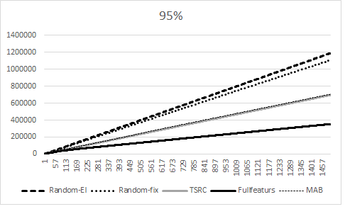
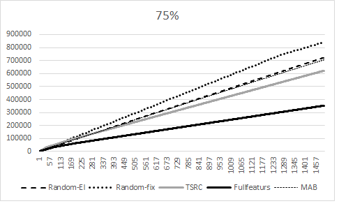
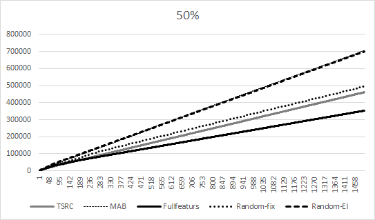
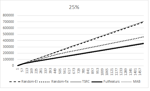
Figure 1: Stationary Environment (Covertype dataset)

Table 3: Non-Stationary Environment

	MAB	Fullfeatures	TSRC	Random-fix	Random-EI	WTSRC
Datasets
Covertype	$69.72\pm 4.30$	$68.54\pm 2.10$	$76.12\pm 2.86$	$80.96\pm 2.19$	$80.71\pm 2.22$	$\textbf{60.56 }\pm\textbf{2.95}$
CNAE-9	$74.34\pm 5.39$	$69.21\pm 2.12$	$71.87\pm 4.5$	$79.87\pm 4.5$	$76.21\pm 1.90$	$\textbf{65.56 }\pm\textbf{1.05}$
Internet Advertisements	$43.99\pm 3.85$	$40.21\pm 1.87$	$42.01\pm 1.79$	$40.04\pm 4.52$	$40.56\pm 1.19$	$\textbf{38.06 }\pm\textbf{0.85}$
Poker Hand	$82.90\pm 4.03$	$82.44\pm 0.43$	$78.86\pm 1.25$	$79.99\pm 1.48$	$79.81\pm 0.48$	$\textbf{77.56 }\pm\textbf{1.79}$

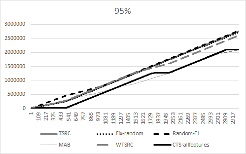
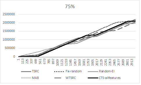
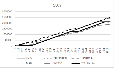
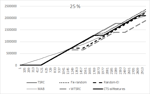
Figure 2: Non-Stationary Environment (Covertype dataset)

In order to simulate a data stream, we draw samples from the dataset sequentially, starting from the beginning each time we draw the last sample. At each round, the algorithm receives the reward 1 if the instance is classified correctly, and 0 otherwise. We compute the total number of classification errors as a performance metric.

We compare our algorithms with the following competing methods:

• Multi-arm Bandit (MAB): this is the standard Thomspon Sampling approach to (non-contextual) multi-arm bandit setting.

• Fullfeatures: this algorithm uses the contextual Thomspon Sampling (CTS) with the full set of features.

• Random-EI: this algorithm selects a Random subset of features of the specified size $d$ at Each Iteration (thus, Random-EI), and then invokes the contextual bandit algorithm (CTS).

• Random-fix: similarly to Random-EI, this algorithm invokes CTS on a random subset of $d$ features; however, this subset is selected once prior to seeing any data samples, and remains fixed.

We ran the above algorithms and our proposed TSRC and WTSRC methods, in stationary and non-stationary settings, respectively, for different feature subset sizes, such as 5%, 25%, 50% and 75% of the total number of features.

In the Figures presented later in this section, we used the parameter, called sparsity, to denote the percent of features that were not selected, resulting into the sparsity levels of 95%, 75%, 50% and 25%, respectively. In the following sections, we will present our results first for the stationary and then for the non-stationary settings.

5.1 Stationary case

Table  2 summarizes our results for the stationary CBRC setting; it represents the average classification error, i.e. the misclassification error, computed as the total number of misclassified samples over the number of iterations. This average errors for each algorithm were computed using 10 cyclical iterations over each dataset, and over the four different sparsity levels mentioned above.

As expected, the CTS algorihtm with the full set of features (Fullfeatures) achieved the best performance as compared with the rest of the algorithms, underscoring the importance of the amount of context observed in an on-line learning setting.

However, when the context is limited, is in the CBRC problem considered in this work, our TSRC approach shows superior performance (shown in bold in Table  2) when compared to the rest of the algorithms, except for the Fullfeatures, confirming the importance of efficient feature selection in the CBRC setting.

Overall, based on their mean error rate, the top three algorithms were TSRC (mean error 49.01%), Random-fix (mean error 55.46%), and MAB (mean error 57.98%), respectively, suggesting that using a fixed randomly selected feature subset may still be a better strategy than not considering any context at all, as in MAB. However, as it turns out, ignoring the context in MAB may still be a better approach than randomly changing the choice of feature at each iteration in Random-EI; the latter resulted into the worst mean error of 61.18%.

5.1.1 Detailed analysis on Covertype dataset

Figure 1 provides a more detailed evaluation of the algorithms for different levels of sparsity, on a specific dataset. Ignoring the Fullfeatures which, as expected, outperforms all methods since it considers the full context, we observe that:

95 % sparsity: TSRC has the lowest error out of all methods, followed tightly by MAB, suggesting that, at a very high sparsity level, ignoring the context (MAB) is similar to considering only a very small (5%) fraction of it. Also, as mentioned above, sticking to the same fixed subset of randomly selected features appears to be better than changing the random subset at each iteration.

75 % sparsity: we observe that Random-EI has a lower error than the Random-fix.

50 % sparsity: TSRC has the lowest error, followed closely by the Random-fix, which implies that, at some levels of sparsity, random subset selection can perform almost as good as our optimization strategy. Again, we observe that Random-fix performs better that the Randon-EI, where the performance of the latter is close to the multi-arm bandit without any context.

25 % sparsity: we observe that TSRC perform practically as good as Fullfeatures, which implies that at this sparsity level, our approach was able to select the optimal feature subset.

5.2 Non-stationary Case

In this setting, for each dataset, we run the experiments for 3,000,000 iterations, where we change the label of class at each 500,000 iteration to simulate the non-stationarity. We evaluate our WTSRC algorithm for the nonstationary CBRC problem against our stationary-setting TSRC method, and against the same five baseline methods we presented before.

Similarly to the stationary case evaluation, the Table  3 reports the mean error over all iterations and over the same for level of sparsity as before. Overall, we observed that the WTSRC performs the best, confirming the effectiveness of using our time-windows approach in a non-stationary on-line learning setting.

Our top three performing algorithms were WTSRC, Fullfeatures and TSRC, in that order, which underscores the importance of the size of the observed context even in the non-stationary on-line learning setting.

5.2.1 Detailed analysis on Covertype dataset

Figure 2 provides a more detailed evaluation of the algorithms for different levels of sparsity, on a specific dataset. The Fullfeatures, as expected, has the same performance on different level of sparsity, since it has the access to all features. We observe that:

95 % sparsity: MAB has the lowest error, as compared with the Random-EI and Random-fix, which implies that, at high sparsity levels, ignoring the context can be better then even considering a small random subset of it.

75 % sparsity: TSRC yields the best result, implying that even in a non-stationary environment, a stationary strategy for best subset selection can be beneficial.

50 % sparsity: both Random-Fix and Randon-EI yield the worst results, implying that random selection is not a good strategy at this sparsity level in non-stationary environment.

25 % sparsity: our nonstationary method, WTSRC, outperforms all other algorithms, demonstrating the advantages of a dynamic feature-selection strategy in a non-stationary environment at relatively low sparsity levels.

6 Conclusions

We have introduced a new formulation of MAB, motivated by several real-world applications including visual attention modeling, medical diagnosis and RS. In this setting, which we refer to as contextual bandit with restricted context (CBRC), a set of features, or a context, is used to describe the current state of world; however, the agent can only choose a limited-size subset of those features to observe, and thus needs to explore the feature space simultaneously with exploring the arm space, in order to find the best feature subset. We proposed two novel algorithms based on Thompson Sampling for solving the CBRC problem in both stationary and non-stationary environments. Empirical evaluation on several datasets demonstrates advantages of the proposed approaches.

7 Acknowledgments

The authors thank Dr. Alina Beygelzimer and Dr. Karthikeyan Shanmugam for the critical reading of the draft manuscript.

References

- Abbasi-Yadkori et al. [2012] Yasin Abbasi-Yadkori, Dávid Pál, and Csaba Szepesvári. Online-to-confidence-set conversions and application to sparse stochastic bandits. In Proceedings of the Fifteenth International Conference on Artificial Intelligence and Statistics, AISTATS 2012, pages 1–9, 2012.
- Agrawal and Goyal [2012] Shipra Agrawal and Navin Goyal. Analysis of thompson sampling for the multi-armed bandit problem. In COLT 2012 - The 25th Annual Conference on Learning Theory, June 25-27, 2012, Edinburgh, Scotland, pages 39.1–39.26, 2012.
- Agrawal and Goyal [2013] Shipra Agrawal and Navin Goyal. Thompson sampling for contextual bandits with linear payoffs. In ICML (3), pages 127–135, 2013.
- Allesiardo et al. [2014] Robin Allesiardo, Raphaël Féraud, and Djallel Bouneffouf. A neural networks committee for the contextual bandit problem. In Neural Information Processing - 21st International Conference, ICONIP 2014, Kuching, Malaysia, November 3-6, 2014. Proceedings, Part I, pages 374–381, 2014.
- Auer et al. [2002] Peter Auer, Nicolò Cesa-Bianchi, and Paul Fischer. Finite-time analysis of the multiarmed bandit problem. Machine Learning, 47(2-3):235–256, 2002.
- Bastani and Bayati [2015] Hamsa Bastani and Mohsen Bayati. Online decision-making with high-dimensional covariates. Available at SSRN 2661896, 2015.
- Bouneffouf and Féraud [2016] Djallel Bouneffouf and Raphaël Féraud. Multi-armed bandit problem with known trend. Neurocomputing, 205:16–21, 2016.
- Carpentier and Munos [2012] Alexandra Carpentier and Rémi Munos. Bandit theory meets compressed sensing for high dimensional stochastic linear bandit. In Proceedings of the Fifteenth International Conference on Artificial Intelligence and Statistics, AISTATS 2012, pages 190–198, 2012.
- Durand and Gagné [2014] Audrey Durand and Christian Gagné. Thompson sampling for combinatorial bandits and its application to online feature selection. 2014.
- Hu and Ogihara [2011] Yajie Hu and Mitsunori Ogihara. Nextone player: A music recommendation system based on user behavior. In ISMIR, pages 103–108, 2011.
- Lai and Robbins [1985] T. L. Lai and Herbert Robbins. Asymptotically efficient adaptive allocation rules. Advances in Applied Mathematics, 6(1):4–22, 1985.
- Langford and Zhang [2008] John Langford and Tong Zhang. The epoch-greedy algorithm for multi-armed bandits with side information. In Advances in neural information processing systems, pages 817–824, 2008.
- Li et al. [2010] Lihong Li, Wei Chu, John Langford, and Robert E. Schapire. A contextual-bandit approach to personalized news article recommendation. CoRR, 2010.
- Mary et al. [2015] Jérémie Mary, Romaric Gaudel, and Philippe Preux. Bandits and recommender systems. In Machine Learning, Optimization, and Big Data - First International Workshop, MOD 2015, pages 325–336, 2015.
- Mnih et al. [2014] Volodymyr Mnih, Nicolas Heess, Alex Graves, et al. Recurrent models of visual attention. In Advances in Neural Information Processing Systems, pages 2204–2212, 2014.
- Tekin et al. [2015] Cem Tekin, Onur Atan, and Mihaela van der Schaar. Discover the expert: Context-adaptive expert selection for medical diagnosis. IEEE Trans. Emerging Topics Comput., 3(2):220–234, 2015.
- Thompson [1933] William R Thompson. On the likelihood that one unknown probability exceeds another in view of the evidence of two samples. Biometrika, 25(3/4):285–294, 1933.
- Villar et al. [2015] Sofía S Villar, Jack Bowden, and James Wason. Multi-armed bandit models for the optimal design of clinical trials: benefits and challenges. Statistical science: a review journal of the Institute of Mathematical Statistics, 30(2):199, 2015.
- Wang et al. [2014] Jialei Wang, Peilin Zhao, Steven CH Hoi, and Rong Jin. Online feature selection and its applications. IEEE Transactions on Knowledge and Data Engineering, 26(3):698–710, 2014.