A model of chromosomal loci dynamics in bacteria as fractional diffusion with intermittent transport.

Abstract

The short-time dynamics of bacterial chromosomal loci is a mixture of subdiffusive and active motion, in the form of rapid relocations with near-ballistic dynamics. While previous work has shown that such rapid motions are ubiquitous, we still have little grasp on their physical nature, and no positive model is available that describes them. Here, we propose a minimal theoretical model for loci movements as a fractional Brownian motion subject to a constant but intermittent driving force, and compare simulations and analytical calculations to data from high-resolution dynamic tracking in E. coli. This analysis yields the characteristic time scales for intermittency. Finally, we discuss the possible shortcomings of this model, and show that an increase in the effective local noise felt by the chromosome associates to the active relocations.

I Introduction

The motion of chromosomal loci of the bacterium Escherichia coli on time scales 0.1–100s shows intriguingly complex patterns Kleckner et al. (2014). These fluctuations contain key evidence on the complex physical nature of the intracellular crowded medium made of genome and cytoplasm Cosentino Lagomarsino et al. (2015); Benza et al. (2012), a stimulating riddle of soft-matter physics with large biological significance. On top of a basal subdiffusive dynamics Javer et al. (2013); Weber et al. (2010a, b), the loci are subject to active forces that have been characterized as both active noise Weber et al. (2012a) and rapid excursions of near-ballistic nature Javer et al. (2014); Fisher et al. (2013); Joshi et al. (2011). The nature of the background motion and of the active relocation is still under debate, and both issues are likely deeply connected with the recent finding that the bacterial cytoplasm shows some glass-like properties Parry et al. (2014).

The rapid relocations emerge as distinct from the subdiffusive background motion of the loci. It is widely accepted that the background motion is compatible with fractional Brownian motion (fBm) or fractional Langevin behavior, i.e. with directionally anti-correlated steps that witness viscoelastic behavior, and with a mobility that is locus- and cell-cycle-dependent Javer et al. (2013); Weber et al. (2010a, 2012a). Consequently, a precise quantification of the fact that rapid relocations deviate from the expected behavior of pure viscoelastic subdiffusion is possible by comparing the behavior of experimental single tracks to a parameter-matched fractional Brownian motion Javer et al. (2014). However, no positive model describing such rapid relocations is currently available. Building such a description is important to address relevant outstanding questions on the nature of the driving force and the relevant time scales that play a role in the process. To this aim, a physical model may be difficult at this stage. The main obstacles are that we still know very little about both the nature of cytoplasmic diffusion Parry et al. (2014); Lampo et al. (2017) and the nature of the nonequilibrium forces driving the chromosome Weber et al. (2012b); Javer et al. (2014). In addition, the contribution of chromosome folding to subdiffusion is an open question Weber et al. (2010b); Lampo et al. (2016); Polovnikov et al. (2017). In this context, a phenomenological model realizing the main pertinent features can be an useful first step Gherardi and Cosentino Lagomarsino (2017).

Importantly, the trajectories showing rapid movements in these data clearly produce superlinear behavior of the mean-square displacement (MSD) Javer et al. (2014). It is well known that in the case of viscoelastic subdiffusion, an object under constant driving force has to produce a sublinear mean-square displacement (drift), in order to follow a fluctuation-dissipation relation Lutz (2001); Barkai and Klafter (1998); Gherardi and Cosentino Lagomarsino (2017). This constraint is realized by the fractional Langevin equation Lutz (2001); Taloni et al. (2010); Kuwada et al. (2013). Thus, given the superdiffusive stretches of motion over a sub-Rouse basal diffusion, it is not clear whether a Stokes-Einstein relation should apply in this situation. The validity of a generalized Einstein relation is ultimately due to the precise nature of the drive, which in this case may act both on the probe and on the environment. For example, a possibility is that the rapid relocations are due to large-scale rearrangements of the chromosome Fisher et al. (2013); Javer et al. (2014).

The recent theoretical literature has focused on active noise, modeled as colored fluctuations violating the fluctuation-dissipation theorem, and on its effect on a Rouse model in a viscoelastic medium Sakaue and Saito (2016); Vandebroek and Vanderzande (2015). However, this framework cannot capture the ballistic stretches observed in the E. coli data. In this system, rapid relocations emerge as distinct from the subdiffusive background motion of the loci, as can be seen by comparing experimental single tracks to a parameter-matched fractional Brownian motion (fBm) Javer et al. (2014).

Here, we take the complementary assumption that active behavior is due to an intermittent force. For simplicity, we give up the description of the polymer degrees of freedom and concentrate on the superposition of subdiffusion with an intermittent driving force. This approach cannot explicitly address the stress propagation between different chromosomal loci, measurable from joint tracking, which is being addressed in the current literature for the equilibrium case Polovnikov et al. (2017); Lampo et al. (2016). Other modeling approaches in the recent literature have explicitly described the dynamics of an active polymer, but represented the active drive as nonthermal noise or as contact of different sets of monomers with two different thermostats Vandebroek and Vanderzande (2015); Grosberg and Joanny (2015); Osmanovic and Rabin (2017). We define a minimal description of the movement of chromosomal loci as a basal fractional Brownian motion superposed to an intermittent process imposing a constant driving force. Comparing with high-resolution tracking data in E. coli, we set out to identify the key behaviors and relevant parameters.

Similar intermittent processes have been proposed in the literature as models for search processes Loverdo et al. (2009) and complex reaction-diffusion Bénichou et al. (2008); Oshanin et al. (2010); Bénichou et al. (2010), as well as for describing the interplay between diffusion and active transport in cells Brangwynne et al. (2009); Lagache and Holcman (2008); Parmeggiani et al. (2004). However, the case of the superposition between subdiffusion and active transport has never been considered, giving a wider motivation to our investigation.

II Model: intermittent transport and subdiffusion.

Fig. 1 illustrates the basic ingredients of the model. A point particle is subject to fractional Gaussian noise Deng and Barkai (2009), which captures the viscoelastic-like subdiffusion Weber et al. (2012a) of chromosomal loci, and to an external driving velocity of constant intensity and orientation, but active only at intermittent intervals.

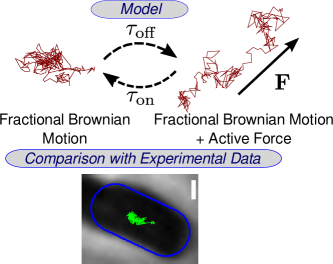
Figure 1: Illustration of the model. An intermittent process switches on and off a constant driving force, acting on top of a basal subdiffusive process with viscoelastic-like behavior, modeled as fractional Brownian motion. The resulting tracks are compared with experimental data from Ref. Javer et al. (2014).

In order to reproduce near-ballistic motion in the driven stretches of motion, this phenomenological model gives up the Einstein relation and uses fractional Brownian motion as a model for the basal subdiffusion. The combination of these ingredients produces the following Langevin-type equation of motion (for each, assumed independent, coordinate $x_{i}$):

$$\dot{x_{i}}(t)=\xi_{i}^{H}(t)+V_{i}\sigma(t)\ ,$$ (1)

where $\mathbf{V}$ is the constant velocity caused by an external force (drag and temperature are incorporated in $\xi_{i}^{H}$). The fractional noise $\xi_{i}^{H}(t)$ is a Gaussian noise with the following correlation properties:

$$\begin{split}\left<\xi_{i}^{H}(t)\right>&=0;\\ \left<\xi_{i}^{H}(t)\xi_{j}^{H}(t^{\prime})\right>&=2D_{\mathrm{app}}H(2H-1)|t-t^{\prime}|^{2H-2}\delta_{ij}\\ &\phantom{=}+4D_{\mathrm{app}}H|t-t^{\prime}|^{2H-1}\delta(t-t^{\prime})\delta_{ij}\ ,\end{split}$$ (2)

where $H$ is the Hurst exponent (or coefficient) and $D_{\mathrm{app}}$ is the apparent diffusion constant. When $H<1/2$ noise at different times is anti-correlated, with power-law relaxation (see Ref. Qian (2003) for a justification of the expressions in Eq. 2). The stochastic process $\sigma(t)$ governing how the external force switches on and off is a standard dichotomous telegraph process, with states 0 and 1. It is specified by the two characteristic switching times $\tau_{\mathrm{on}}=w\tau_{0}$ and $\tau_{\mathrm{off}}=(1-w)\tau_{0}$ bringing the system from the on state to the off state and viceversa, respectively. In what follows, when most convenient, we use the variables $w$ (average fraction of time in the “on” state) and $\tau_{0}$ (average length of a full “off”-“on”-“off” cycle) to characterize this process.

The probability $P_{+}$ and $P_{-}$ that the force is switched on or off at time $t$, i.e. that $\sigma(t)=1$ or $\sigma(t)=0$ respectively, obeys the following master equation:

$$\partial_{t}P_{\pm}(t)=\mp\frac{P_{+}(t)}{w\tau_{0}}\pm\frac{P_{-}(t)}{(1-w)\tau_{0}}\ .$$

In the stationary state of the telegraph process the probability of the “on” state equals $P_{+}^{s}=w$ (clearly, the probability of the “off” state is $P_{-}^{s}=1-w$). We assume this stationary state as the initial condition in what follows.

III Results

Analytical form of the mean-square displacement in presence of active forces

Our first result is the derivation of an exact analytical expression for the mean-square displacement of the model. As we will show, this expression is very useful to compare the model to experimental data.

The equation of motion of the process, Eq. (1), can be integrated formally, obtaining

$$\Delta x_{i}(\tau)=\Delta x_{i,\mathrm{fBm}}(\tau)+V_{i}T_{\mathrm{on}}(\tau)\ ,$$

where $\Delta x_{i}(\tau)$ stands for the net change of a coordinate from the initial condition, $\Delta x_{i,\mathrm{fBm}}(\tau)$ is the contribution of the fractional noise, and $T_{\mathrm{on}}(\tau)=\int_{0}^{\tau}\sigma(t)\,dt$ is a random variable representing the time during which the active force is switched on in the interval $[0,\tau]$. Considering the square of this expression and averaging leads to an expression for the mean-square displacement. By observing that mixed terms average to zero, due to the random force and the telegraph process being independent, and that the mean signed step of a fractional Brownian motion is null, we obtain

$$\mathrm{MSD}(\tau)=2dD_{\mathrm{app}}\tau^{2H}+V^{2}\langle T_{\mathrm{on}}^{2}(\tau)\rangle\ ,$$ (3)

where $d$ is the dimensionality of the space. We choose $d=2$, as the nature of essentially all experimental tracking data is intrinsically two-dimensional, although loci move in three dimensions.

The computation of $\langle T_{\mathrm{on}}^{2}(\tau)\rangle$ relies on the fact that the correlation function for a telegraph process is known:

$$\begin{split}\langle\sigma(t_{1})\sigma(t_{2})\rangle&=\langle\sigma_{\mathrm{s}}\rangle^{2}+\mathrm{Var}\left(\sigma_{\mathrm{s}}\right)\exp\left(-\frac{\left\lvert t_{2}-t_{1}\right\rvert}{\tau_{\mathrm{c}}}\right)\\ &=w^{2}+w(1-w)\exp\left(-\frac{\left\lvert t_{2}-t_{1}\right\rvert}{\tau_{\mathrm{c}}}\right)\ ,\end{split}$$

where we used the shorthand $\tau_{\mathrm{c}}=w(1-w)\tau_{0}$ for the time scale in the exponential. The second equality uses the analytical results for the average and the variance of $\sigma$ in the stationary state. The mean square waiting time can then be obtained by double integration as $\langle T_{on}^{2}(\tau)\rangle=\iint_{\Omega}\langle\sigma(t_{1})\sigma(t_{2})\rangle\,\mathrm{d}t_{1}\mathrm{d}t_{2}$ within the square $\Omega=\{0\leq t_{1}\leq\tau,0\leq t_{2}\leq\tau\}$. By substituting the result into Eq. (3) we obtain the final analytical expression for the mean-square displacement in presence of the switching active force,

$$\begin{split}\mathrm{MSD}(\tau)&=2dD_{\mathrm{app}}\tau^{2H}+V^{2}w^{2}\tau^{2}\\ &+2V^{2}\frac{\tau_{0}^{2}}{w(1-w)}\left(e^{-\tau/\tau_{\mathrm{c}}}-1+\frac{\tau}{\tau_{\mathrm{c}}}\right).\end{split}$$ (4)

For small lag times, namely when $\tau\ll\tau_{\mathrm{c}}$, the linear term in parentheses cancels out with the term coming from the first-order expansion of the exponential, giving

$$\mathrm{MSD}(\tau)\approx V^{2}w^{2}\tau^{2}+2dD_{\mathrm{app}}\tau^{2H}\ .$$ (5)

The above formula shows that in the limit of small lag times, since the lower power $2H$ dominates, the process is increasingly similar to a fractional Brownian motion with Hurst exponent $H$.

Quantitative agreement between model and data

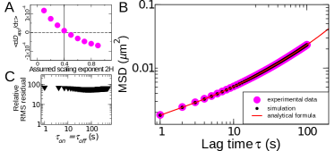
Figure 2: The model reproduces the mean-square displacement of experimental data allowing to fix all model parameters. A. Determination of the scaling exponent $2H$ of the background subdiffusion. Purple circles are the mean of the discrete derivative (1s steps) of $D_{\mathrm{app}}:=\left\langle r^{2}(\tau)/t^{2H}\right\rangle$, for values of lag time below 10 seconds, where the averages are not affected by the influence of ballistic stretches Javer et al. (2014). Since a well-defined $D_{\mathrm{app}}$ should not vary with time scale, the optimal estimated value for the scaling exponent $H\simeq 0.2$ is obtained when the plot crosses zero. B: Large purple circles represent mean-square displacement vs lag time for the data on the Ori3 locus in Ref. Javer et al. (2014) (error bars, SE, are smaller than symbols). Red line and small black circles are, respectively, a fit with the analytical formula, Eq. (4), and simulation results obtained with the parameter values fixed by the fits (reported in table 1A). $2H=0.41$ is fixed from the analysis shown in panel A. C: Fits with $w=1/2$ cannot reproduce the data. The plot shows the ratio of the RMS residual of fits imposing $w=1/2$ to the RMS residual of the unconstrained fit shown in panel B, for different values of the time scale. The ratio between the two values is in the range 50–70.

We used the analytical expression for the mean-square displacement to fix model parameters from experimental data. In order to do so, we first determined separately an optimal value of the subdiffusion exponent $2H$ for the background properties. To obtain this value we defined a procedure based on the fact that for time lags below $\sim 10$s, the mean-square displacements are compatible with pure subdiffusion Javer et al. (2013, 2014). Hence, by assuming varying values of $H$, we looked at the coherence of $4D_{\mathrm{app}}(\tau):=\mathrm{MSD}(\tau)/\tau^{2H}$, by taking the mean of its derivative with respect to $\tau$ and verifying where it crossed zero (Fig. 2A). This procedure gives a value $2H\simeq 0.4$, in line with previous studies focused on the subdiffusion of E. coli chromosomal loci Weber et al. (2010a); Javer et al. (2013). All our fits (including the ones described below) were performed with a nonlinear least-squares Marquardt-Levenberg algorithm minimizing the chi-square residual, weighted on the standard errors of the input data.

$$\begin{array}[]{r|ccccc|cc}\mathrm{param.}&\boldsymbol{2H}&\boldsymbol{4D_{\textrm{app}}}&\boldsymbol{V}&\boldsymbol{\tau_{\mathrm{on}}}&\boldsymbol{\tau_{\mathrm{off}}}&\boldsymbol{\tau_{0}}&\boldsymbol{w}\\ \mathrm{units}&\mathrm{none}&\nicefrac{\mathrm{{\mu m}^{2}}}{\mathrm{{s}^{2H}}}&\nicefrac{\mathrm{\mu m}}{\mathrm{s}}&\mathrm{s}&\mathrm{s}&\mathrm{s}&\mathrm{none}\\ \hline\cr\mathrm{fits:}\;\;\mathrm{A}&\approx 0.4&0.00182&0.023&7&427&434&0.016\\ \mathrm{B}&0.40&0.00180&0.024&7.0&443&450&0.016\\ \mathrm{C}&0.404&0.00182&0.020&7.7&412&420&0.018\\ \mathrm{D}&0.48&0.00167&0.005&27&377&404&0.067\\ \mathrm{E}&0.79&0.00063&\mathrm{NA}&\mathrm{NA}&\mathrm{NA}&\mathrm{NA}&\mathrm{NA}\\ \hline\cr\end{array}$$

Table 1: A: Parameter values for the theoretical curve and simulations of the constrained model fit shown in Fig. 2. B: Parameter values from the alternative fitting procedure using the subtraction of the subdiffusing contribution to the MSD, shown in Fig. 3. C: Parameter values for the systematic 4-parameter fit. D: Parameter values for the joint model fit considering the end-to-end distance distribution. E: Parameters of the best-fitting fBm. (Estimated errors affect the last displayed digits.)

Subsequently, we performed a 4-parameter fit of the data with Eq. (4), thus fixing $\tau_{0}$, $w$, $V$, and $D_{\mathrm{app}}$. The parameter values obtained are reported in Table 1A. We also verified that direct simulations of the model with this choice of parameters agreed with the data. Figure 2B shows that the agreement between the mean-square displacement curves given by the analytical formula, by simulations of the model, and by data is excellent. The ingredients of the model are therefore sufficient to reproduce the experimental observations on the mean-square displacement.

Importantly, a model with a reduced parameter space, where the two characteristic switching times (on and off) are equal, cannot reproduce the mean-square displacement of the experimental data. We considered a constrained fit with $w=1/2$, by varying this parameter in a wide range of values. The results, shown in Fig 2C, clearly indicate that the performance of this fit is much worse. Intuitively, if $\tau_{\mathrm{on}}=\tau_{\mathrm{off}}$ the number of tracks in which the force is off all the time (i.e., the purely subdiffusive ones) equals the number of tracks in which it is always switched on. However, it is clear that the tracks showing simple subdiffusive behavior are much more common in the data than the tracks dominated by ballisitic-like drift Javer et al. (2014).

Subtraction of subdiffusive noise unveils superdiffusive behavior in the data

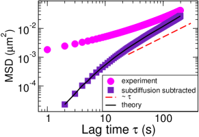
Figure 3: A subtraction procedure based on the model confirms the superdiffusive nature of the observed rapid chromosomal movements. Purple circles are mean-square displacement vs lag time from the same data as in Fig. 1. Indigo squares are obtained by subtracting the background fBm contribution from the mean-squared displacement [Eq. (3)]. The remaining contribution to the mean-square displacement is super-linear (the red dashed line is the linear scaling), as predicted by Eq. (4), consistent with the hypothesis of intermittent active relocations.

As a consistency check of the agreement between model and data, we considered the possibility of disentangling contributions to the mean-square displacement from active force and subdiffusion [Eqs (3) and (4)].

We used this property to define an alternative analysis of the experimental MSD. First, we fixed $D_{\textrm{app}}$ and $H$ by fitting the mean-square displacement for time scales below $10$s averaged on all tracks. We then considered the subtracted MSD, calculated as $\mathrm{MSD}(\tau)-2dD_{\mathrm{app}}\tau^{2H}$, and fitted it with a polynomial function (assuming the regime for the lag times $\tau\gg\tau_{0}$). Remarkably, this procedure leads to very similar parameter values as the blind fit (Table 1B). By comparison, the best-fitting fractional Brownian motion performs much worse (Table 2). The fact that the two procedures lead to essentially the same parameters suggests that the parameter region that can reproduce the experimental data is localized and univocal, and the existence of a null manifold or multiple solutions is unlikely. In order to further support this statement, we performed systematic 4-parameter fits of $\tau_{0}$, $w$, $V$, and $D_{\mathrm{app}}$, by varying $2H$ in the interval $(0,1)$. Comparing the goodness-of-fit scores confirmed that there is a single global best fit, corresponding to $2H=0.404$ (parameters are reported in Table 1C).

$$\begin{array}[]{c | c c c }&\textrm{Best-fit fBm}&\textrm{Constr. fit}&\textrm{Joint fit}\\ \hline\cr\textrm{Reduced RMS}&$5.9\text{\times}{10}^{-03}$&$2\text{\times}{10}^{-06}$&$7.6\text{\times}{10}^{-05}$\\ \end{array}$$

Table 2: Comparison of the goodness-of-fit scores for the MSD in the data with the best-fitting simple fBm model, with the constrained active-force model fit, and with the joint fit keeping into account the end-to-end distance distribution (Table 1D). The reduced RMS is defined as the chi-square residual divided by the number of degrees of freedom.

Model predictions beyond mean-square displacement

So far we considered constrained fits based exclusively on the MSD curves fixing a priori $H$ or both $D_{\textrm{app}}$ and $H$ based on the short-time behavior, which should estimate the background process. This constrained procedure fixes all parameters, and we verified that the model greatly improves the best fit of MSD vs lag time compared to a normal fBm (Table 2), by comparing their reduced chi-square. These clear quantitative differences mirror the important qualitative difference between the model and the normal fBm. Indeed, the latter model simply cannot reproduce the MSD curves observed in the data, which are visibly bent in log-log scale.

However, while the ensemble-averaged MSD is useful to establish that an improved model is needed, this mean quantity is notoriously non discriminating. Importantly, the active-force model also leads to different predictions for single-track properties, so it could reproduce the data more effectively than a simple fBm even if its performance on the MSD fit were equivalent. Many models, each with a distinct physical mechanism, may predict the same (bent) ensemble-averaged MSD. For example, a “tempered” fBm Meerschaert and Sabzikar (2013) (with a time cutoff in the noise autocorrelation function) would crossover to diffusive behavior at a prescribed time scale. However, this model would not be able to show super-diffusive behavior on a subset of tracks, as it is visible in the data.

Hence, more detailed comparisons with tracking data are useful. We considered the single-track end-to-end distance, and we verified that this gave equivalent result to an effective drift velocity based on the projection of the end-to-end distance on the main track axis used in previous work Javer et al. (2014) (not shown). All these observables are independent predictions from the model (whose parameters are fixed by the fitting procedure of the ensemble-averaged MSD) and can be matched precisely in track length and sampling to experimental data. Additionally, these quantities should discriminate models that predict near-ballistic behavior for a subset of tracks.

Fig. 4A shows that the prediction for the distribution of the track end-to-end distance $R_{\mathrm{e}}$ improves the estimate of the tails with respect to the background fBm, as well as with respect to a best-fit fBm. Fig 4B shows mean-square displacements as a function of lag times, both for all tracks and as conditional averages on the subset of tracks whose $R_{\mathrm{e}}$ is in the top $30\%$ and bottom $70\%$ of the distribution shown in Fig 4A.

The agreement is remarkable, since the model is adjusted only through a fit of the mean-square displacement, so that the agreement has to be regarded as an independent prediction. However, the active force model tends to overestimate the tail of the end-to-end distance and to underestimate the diffusivity of tracks where the ballistic transport is not active. The former effect becomes evident at long lag times, while the latter appears at short lags (as visible in Fig. 4AB). The best-fitting fBm, while not being able to capture the tails present in the data, appears to give better a compromise (and is definitely more parameter-poor) between bulk behavior and tails. However, this model cannot be considered a viable alternative, since its performance is clearly much worse in fitting the ensemble-averaged MSD, and it gives an unrealistic value of the exponent $2H$, close to 0.8 (Table 1E).

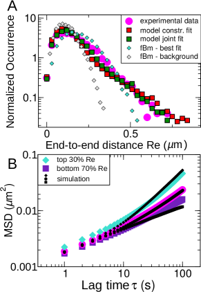
Figure 4: The model predicts correctly the qualitative behavior of single-track end-to-end distances and conditional mean-square displacements. A: Distribution of the track end-to-end distance $R_{\mathrm{e}}$ in experimental data (purple circles), the intermittent active force model (black filled smaller circles) and fractional Brownian motion (open smaller circles). Simulations have been matched with experimental data, both in number and length of tracks (parameters shown in Tab. 1). B: Conditional averages of mean-square displacements on tracks within a given percentile of $R_{\mathrm{e}}$ (diamonds, top $30\%$, and squares, bottom $70\%$ shown as example) show qualitative agreement and some quantitative discrepancies. Circles are the overall MSD average shown in Fig. 2.

Joint optimization of model parameters on end-to-end distance

To improve the agreement of model with single-track data, we performed a joint fit where, instead of fixing the parameters purely based on the analytical MSD fit, we also considered explicitly the long-time end-to-end distances. Specifically, we considered all the best fits of the model at fixed $D_{\mathrm{app}}$ and $H$, for a grid of these values, and we evaluated the manifold of residuals on the histogram of end-to end distance $R_{\mathrm{e}}$. The parameters for the optimal fit with these criteria are given in Table 1D, and the resulting distribution of $R_{\mathrm{e}}$ is plotted in Fig. 4A. Additionally, Table 2 shows that the trade-off in the residuals of the MSD for this fit is acceptable, and gives a better agreement with the data than the best-fit fBm.

One possible additional source of error overestimating the tails of the end-to-end track length distribution is the fact that the model assumes a constant force in direction and orientation for the active process, which is not plausible in the data. The discrepancy between model and data is expected to occur when the force is active more than once in a single track. With the model parameters, a simple estimate leads to the expectation for this to happen in 2-4% of the tracks (which are 100s long), and thus we can predict that this factor only affects the tail of the end-to-end distance distribution in this range of percentiles.

Different chromosomal loci have coordinate-specific parameters

The fitting procedures defined above are applicable to data from different loci. We applied the constrained fit to all loci from the datasets in refs.Javer et al. (2013, 2014) where 1s lag data were available. The results are shown in Fig. 5. We can obtain a rough estimate of the errors in these results by considering the range of variability of the fits analyzed above (Tab. 1), which is of order $10\%$ for $V$, $\tau_{\mathrm{on}}$, and $\tau_{\mathrm{off}}$: the symbol size in Fig. 5 reflects the estimated errors. The results indicate a clear trend for the typical velocity $V$, which follows an opposite trend to $\tau_{\mathrm{on}}$. Since the anticorrelation between $V$ and $w$ (Eq. (5)) is intrinsic of the model, one may interpret this trend as the variation of a single physical parameter. Conversely, the characteristic off-time $\tau_{\mathrm{off}}$ does not show a clear trend, and tends to become very large in some loci. The differences in the estimated process observed for different chromosomal loci can be interpreted as differences in the physical organization of the chromosome or in the action of the active drive Javer et al. (2013, 2014); Fisher et al. (2013). In one specific case, the Left1 locus, the algorithm used for the fit locates a very shallow minimum for $\tau_{\mathrm{off}}$, so it is difficult to pinpoint a precise value for this parameter. We believe that the applicability of the model to this particular locus is debatable (the corresponding points are highlighted in Fig. 5. The values for the apparent diffusion constant fits of the loci (not shown) are coherent with the trends found in ref. Javer et al. (2013).

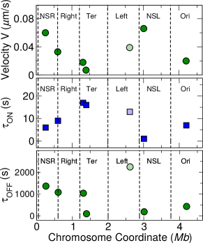
Figure 5: Parameter values for different chromosomal loci. Top panel: typical velocity of excursions $V$. Middle panel: characteristic time $\tau_{\mathrm{on}}$. Bottom panel: characteristic time $\tau_{\mathrm{off}}$. The results of the less reliable fit of the Left1 locus are shown in faded colors. The strong differences observed for different chromosomal loci can be interpreted as local differences in the physical organization or in the action of the active driveJaver et al. (2013, 2014). (Estimated errors are around the size of the points.)

Active movements carry additional noise

Finally, we addressed a second shortcoming of the model, visible in Fig. 4. Namely, the predictions of the conditional mean-square displacements for tracks with end-to-end distance $R_{\mathrm{e}}$ in the higher or lower tails of the distribution show relevant differences between model and data (Fig. 4B). In particular, the mean-square displacement in the model is essentially independent of track end-to-end distance $R_{\mathrm{e}}$ at short lag times, while the data are not.

The fact that the model should behave this way is evident from Eq. (1) and (5). At short time lags, fractional Brownian motion dominates the displacement, and this process occurs at fixed noise level. Hence, the model at short lags behaves precisely as an fBm with fixed noise amplitude, and therefore it cannot show the variation in diffusivity found in the data. In other words, for short enough lags, even trajectories where the driving is switched on should show the same amount of subdiffusion.

Instead, the lack of agreement between data and model suggests that active movements may be also characterized by increased noise levels, on top of a directional driving force. Physically, this could be due to heterogeneity in the diffusion coefficient, related to the active excursions (see below) Wang et al. (2012). In order to explore this hypothesis, we defined a variant of the model, where active movements are also subject to increased noise levels. This is described by the following equation of motion

$$\dot{x_{i}}(t)=\left[1+q\sigma(t)\right]\xi_{i,fBm}(t)+V_{i}\sigma(t)\ ,$$ (6)

where $q$ describes a (nonthermal) contribution to noise amplitude in presence of active motion, and the other quantities are identical to Eq. (1). The extra noise parameter $q$ determines an increased diffusivity in presence of the driving process and is determined by a fit of the extended model. This modified model makes it qualitatively possible for the MSD to vary with track end-to-end distance, as observed in the data. Fig. 6A shows that simulations of this model variant reproduce the short time-lag changes in the conditional mean-square displacement for trajectories with varying end-to-end distance. To better capture the specificity of this model variant, Fig. 6B shows the conditional mean-square displacement at 1s time lag for tracks in the bottom and top tail of the end-to-end distance distribution, plotted as a function of end-to-end distance percentile. In this plot, the value of the $x$ axis refers to the $x-\%$ top and bottom tail of the track end-to-end distance distribution. Hence, the plot tests the consistency of the agreement between model and data if the cutoff is shifted lower or higher in the end-to-end distance distribution. Comparison of data with simulations of both models shows that only the variant with modified noise during active stretches is able to modulate the diffusivity at short lags.

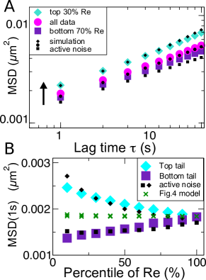
Figure 6: Additional diffusivity of active excursions. A: the model variant including active noise (black filled symbols) fully captures the conditional mean-square displacement at short time lags of experimental data (large filled symbols), for trajectories that fall in different percentiles of end-to-end distance $R_{\mathrm{e}}$ (top 30% $R_{\mathrm{e}}$, diamonds versus bottom 70%, squares). B: Conditional mean-square displacement at 1s time lag computed as a function of end-to-end distance percentile, and compared with simulations. Model parameters in Table 1B, $q=0.78$.

IV Discussion and Conclusions.

We considered a phenomenological model of subdiffusing particles performing fractional Brownian motion and subject to intermittent ballistic excursions and analyzed the validity of this description for chromosomal loci movements. The comparison procedure allows to evaluate the relevant time scales and to dissect some specific features of the data. The model defined here potentially has a wider range of applications, including eukaryotic chromosomal loci, where similar active phenomena have been reported, and may or may not have the same interpretation Bronshtein et al. (2016); Bronstein et al. (2009).

The first outcome of the model concerns the estimated intensity and typical time scales of the active movements. Different approaches and fits all suggest that the characteristic times of active relocations span a few seconds, while the typical waiting times between activations are of the order of a few hundred seconds. Both processes occur below the typical time scales of a cell interdivision time (tens of minutes to hours) and hence should be observable in every cell, and overlap with the key cell processes of replication and chromosome segregation. Additionally, the typical speeds of the relocations are estimated to be slightly over one micron per minute. These figures are in agreement with previous reports Kleckner et al. (2014); Javer et al. (2014); Fisher et al. (2013); Joshi et al. (2011), but the present work is a systematic attempt to capture these time scales quantitatively using a theoretical framework.

A second important feature of the model is its ability to generate nontrivial testable predictions. We first used the mean-square displacement to fix the parameters, and then considered the behavior of the distributions of track end-to-end distances and the conditional mean-square displacements. The model captures the behavior of these quantities in experimental data better than the best-fit fBm. However, some discrepancies exist both at short and at long time scales. A model fit purely based on the mean-square displacement behavior tends to overestimate the mobility of the tracks where the transport is switched on, and this effect is particularly visible at long time scales. To compensate for this behavior, we defined a fitting procedure that also takes into account the end-to-end distance distributions at these long time scales, which gives a more satisfactory agreement. Additional differences at long time scales may be attributed to simplifying hypotheses in the definition of the model, such as the assumption of a single relevant scale for the diving force and of a simple telegraph process for the force switch. Focusing on short time scales, we have isolated an increased diffusivity of faster-moving foci as a potential relevant ingredient (see below).

Notably, we have compared different models with different number of parameters. Admittedly, it may seem unsurprising that models with more parameters give better results. The important feature to note is that each extension considered here is defined based on the ability to capture a different qualitative behavior. For example, the intermittent force model can produce MSD curves that are bent in a log-log scale, which is impossible with a normal two-parameter fBm. Alternative models that may include this qualitative feature (such as a tempered fBm) would still entail adding more parameters. Equally, the model variant with additional noise in active movements can reproduce the qualitative feature of increased diffusivity in tracks with increasing end-to-end distance, which is not possible to reproduce in the simpler variant of the model.

Our analysis of different fitting procedures (compared in Table 1) can be used to produce a rough estimate of the errors on these parameters. Considering the values of the different fits, we expect the errors to be between 5% and 10% for the typical velocity $V$, and the transition time scales $\tau_{\mathrm{on}}$ and $\tau_{\mathrm{off}}$, and less than $1\%$ for the scaling exponent $H$ and the apparent diffusion constant $D_{\mathrm{app}}$.

It is interesting to compare the value of the inferred model parameters with some rates and durations of relevant biological processes at play. The characteristic times for active relocations (5–10 s) agree well with the time scales of the pulses of density shift Fisher et al. (2013) observed along the nucleoid ($\sim$5 s). These pulses were found to occur at about 20 minutes intervals, to be compared with the 7-23 minutes of the fitted characteristic off times. From our fits, these values appear to be locus dependent, and to be closer to 20 minutes in the Right-Ter arm of the chromosome. Finally, the characteristic speed of the active process, about a micron per minute, compares well with the speed of these fast processes Javer et al. (2014); Joshi et al. (2011); Fisher et al. (2013), happening at much faster time scales than the average speed of segregation, which is on the scale of microns per hour. These characteristic times vary along the chromosome, coherently with previous findings Javer et al. (2014, 2013) that suggested differential organization and/or local noise along the chromosomal coordinates. For some loci, the characteristic off-time of the process becomes very large, indicating that the active excursions could become extremely rare.

Finally - the comparison of model predictions and data leads us to the conclusion that active relocation also carries increased noise levels. Specifically, a model where noise amplitude is constant in presence of active excursions cannot reproduce the increase in diffusivity at short lag times observed in experimental data. This suggests that the processes generating the active relocations are concurrent with the noise-increasing processes. The microscopic interpretation of this result is unclear. One possibility is that this increased diffusivity is due to nonthermal active fluctuations Weber et al. (2012b). However, nonthermal random forces are expected to dominate at long time lags. The noise increase has been proven to be ATP-dependent, but not associated to any specific process such as the activity to DNA gyrase (Topoisomerase favoring relaxation of positive supercoiling) or depolymerization of MreB (cell wall biosynthesis), and is only weakly linked to RNA polymerase activity. Active relocations have been previously interpreted as relaxation of stress (generated by process such as DNA replication and transcription) due to release of internal tethering interactions (e.g., by bridging proteins such as H-NS and Fis or condensins such as MukBEF) Kleckner et al. (2014); Javer et al. (2014); Fisher et al. (2013). This kind of motion is not necessarily associated to increased noise, because the stress-release events might be well-separated temporally from the stress-generating ones.

Another possibile interpretation (complementary to the previous one) of the increased mobility in presence of active movements might explain this behavior. This is related to the reported glassy properties of the cytoplasm system Parry et al. (2014), which should also affect the nucleoid. In this framework, active relocation might cause a fluidization effect, releasing local portions of cytoplasm and nucleoid from “cages” where they are otherwise confined with limited mobility. In this case, the differential noise would be due to heterogeneity in the sub-diffusion process Wang et al. (2012, 2009). Possibly more general sources of heterogeneity than glassyness could also lead to similar effects. Such kind of disorder has been recently implicated for the motion of cytoplasmic particles Lampo et al. (2017). A more precise dissection of such hypothesis requires a theoretical approach that incorporates explicitly the more complex physical ingredient of crowding and glassy behavior.

V Acknowledgments

We are grateful to Pietro Cicuta, Kevin Dorfman, Alessandro Taloni for helpful discussions. This work was supported by the International Human Frontier Science Program Organization, grant RGY0070/2014. MT is grateful for the financial support of the EU-Horizon2020 IRSES program DIONICOS (612707).

References

- Kleckner et al. (2014) N. Kleckner, J. K. Fisher, M. Stouf, M. A. White, D. Bates, and G. Witz, Curr Opin Microbiol 22, 127 (2014).
- Cosentino Lagomarsino et al. (2015) M. Cosentino Lagomarsino, O. Espéli, and I. Junier, FEBS Lett 589, 2996 (2015).
- Benza et al. (2012) V. Benza, B. Bassetti, K. Dorfman, V. Scolari, K. Bromek, P. Cicuta, and M. Cosentino Lagomarsino, Rep. Prog. Phys. 75, 076602 (2012).
- Javer et al. (2013) A. Javer, Z. Long, E. Nugent, M. Grisi, K. Siriwatwetchakul, K. D. Dorfman, P. Cicuta, and M. Cosentino Lagomarsino, Nat. Commun. 4, 3003 (2013).
- Weber et al. (2010a) S. C. Weber, A. J. Spakowitz, and J. A. Theriot, Phys. Rev. Lett. 104, 238102 (2010a).
- Weber et al. (2010b) S. C. Weber, J. A. Theriot, and A. J. Spakowitz, Phys. Rev. E 82, 011913 (2010b).
- Weber et al. (2012a) S. C. Weber, M. A. Thompson, W. E. Moerner, A. J. Spakowitz, and J. A. Theriot, Biophys. J. 102, 2443 (2012a).
- Javer et al. (2014) A. Javer, N. J. Kuwada, Z. Long, V. G. Benza, K. D. Dorfman, P. A. Wiggins, P. Cicuta, and M. C. Lagomarsino, Nat Commun 5, 3854 (2014).
- Fisher et al. (2013) J. K. Fisher, A. Bourniquel, G. Witz, B. Weiner, M. Prentiss, and N. Kleckner, Cell 153, 882 (2013).
- Joshi et al. (2011) M. C. Joshi, A. Bourniquel, J. Fisher, B. T. Ho, D. Magnan, N. Kleckner, and D. Bates, Proc. Natl. Acad. Sci. USA 108, 2765 (2011).
- Parry et al. (2014) B. R. Parry, I. V. Surovtsev, M. T. Cabeen, C. S. O’Hern, E. R. Dufresne, and C. Jacobs-Wagner, Cell 156, 183 (2014).
- Lampo et al. (2017) T. J. Lampo, S. Stylianidou, M. P. Backlund, P. A. Wiggins, and A. J. Spakowitz, Biophysical Journal 112, 532 (2017).
- Weber et al. (2012b) S. C. Weber, A. J. Spakowitz, and J. A. Theriot, Proc. Natl. Acad. Sci. USA 109, 7338 (2012b).
- Lampo et al. (2016) T. J. Lampo, A. S. Kennard, and A. J. Spakowitz, Biophysical journal 110, 338 (2016).
- Polovnikov et al. (2017) K. Polovnikov, M. Gherardi, M. Cosentino Lagomarsino, and M. Tamm, arXiv:1703.10841 (2017).
- Gherardi and Cosentino Lagomarsino (2017) M. Gherardi and M. Cosentino Lagomarsino, Procedures for model-guided data analysis of chromosomal loci dynamics at short time scales, edited by O. Espeli, Methods in Molecular BIology, Vol. The Bacterial Nucleoid - Methods and Protocols (Springer Publishing Company, Incorporated, 2017).
- Lutz (2001) E. Lutz, Phys. Rev. E 64, 051106 (2001).
- Barkai and Klafter (1998) E. Barkai and J. Klafter, Physical review letters 81, 1134 (1998).
- Taloni et al. (2010) A. Taloni, A. Chechkin, and J. Klafter, Physical review letters 104, 160602 (2010).
- Kuwada et al. (2013) N. J. Kuwada, K. C. Cheveralls, B. Traxler, and P. A. Wiggins, Nucleic Acids Res. 41, 1 (2013).
- Sakaue and Saito (2016) T. Sakaue and T. Saito, Soft Matter (2016).
- Vandebroek and Vanderzande (2015) H. Vandebroek and C. Vanderzande, Phys. Rev. E 92, 060601 (2015).
- Grosberg and Joanny (2015) A. Y. Grosberg and J.-F. Joanny, Phys. Rev. E 92, 032118 (2015).
- Osmanovic and Rabin (2017) D. Osmanovic and Y. Rabin, Soft Matter 13, 963 (2017).
- Loverdo et al. (2009) C. Loverdo, O. Bénichou, M. Moreau, and R. Voituriez, Phys Rev E Stat Nonlin Soft Matter Phys 80, 031146 (2009).
- Bénichou et al. (2008) O. Bénichou, C. Loverdo, M. Moreau, and R. Voituriez, Phys Chem Chem Phys 10, 7059 (2008).
- Oshanin et al. (2010) G. Oshanin, M. Tamm, and O. Vasilyev, The Journal of Chemical Physics 132, 235101 (2010).
- Bénichou et al. (2010) O. Bénichou, D. Grebenkov, P. Levitz, C. Loverdo, and R. Voituriez, Phys Rev Lett 105, 150606 (2010).
- Brangwynne et al. (2009) C. P. Brangwynne, G. H. Koenderink, F. C. MacKintosh, and D. A. Weitz, Trends Cell Biol 19, 423 (2009).
- Lagache and Holcman (2008) T. Lagache and D. Holcman, Phys Rev E Stat Nonlin Soft Matter Phys 77, 030901 (2008).
- Parmeggiani et al. (2004) A. Parmeggiani, T. Franosch, and E. Frey, Phys. Rev. E 70, 046101 (2004).
- Deng and Barkai (2009) W. Deng and E. Barkai, Phys. Rev. E 79, 011112 (2009).
- Qian (2003) H. Qian, “Processes with long-range correlations,” (Springer Berlin Heidelberg, 2003) Chap. Fractional Brownian Motion and Fractional Gaussian Noise.
- Meerschaert and Sabzikar (2013) M. M. Meerschaert and F. Sabzikar, Statistics & Probability Letters 83, 2269 (2013).
- Wang et al. (2012) B. Wang, J. Kuo, S. C. Bae, and S. Granick, Nature materials 11, 481 (2012).
- Bronshtein et al. (2016) I. Bronshtein, I. Kanter, E. Kepten, M. Lindner, S. Berezin, Y. Shav-Tal, and Y. Garini, Nucleus 7, 27 (2016).
- Bronstein et al. (2009) I. Bronstein, Y. Israel, E. Kepten, S. Mai, Y. Shav-Tal, E. Barkai, and Y. Garini, Phys. Rev. Lett. 103, 018102 (2009).
- Wang et al. (2009) B. Wang, S. M. Anthony, S. C. Bae, and S. Granick, Proceedings of the National Academy of Sciences of the United States of America 106, 15160 (2009).