Random growth lattice filling model of percolation: a crossover from continuous to discontinuous transition

Abstract

A random growth lattice filling model of percolation with touch and stop growth rule is developed and studied numerically on a two dimensional square lattice. Nucleation centers are continuously added one at a time to the empty sites and the clusters are grown from these nucleation centers with a tunable growth probability $g$. As the growth probability $g$ is varied from $0$ to $1$ two distinct regimes are found to occur. For $g\leq 0.5$, the model exhibits continuous percolation transitions as ordinary percolation whereas for $g\geq 0.8$ the model exhibits discontinuous percolation transitions. The discontinuous transition is characterized by discontinuous jump in the order parameter, compact spanning cluster and absence of power law scaling of cluster size distribution. Instead of a sharp tricritical point, a tricritical region is found to occur for $0.5<g<0.8$ within which the values of the critical exponents change continuously till the crossover from continuous to discontinuous transition is completed.

I Introduction

A new era in the study of percolation has started in the recent past developing a series of new models epj223 ; Saberi20151 ; Boccaletti20161 such as percolation on growing networks PhysRevE.64.041902(2001) , percolation in the models of contagion PhysRevLett.92.218701(2004) ; PhysRevE.70.026114(2004) , $k$-core percolation epl73.560(2006) ; *PhysRevE.93.062302, explosive percolation Achlioptas1453 ; *PhysRevLett.103.045701; *Cho20131185, percolation on interdependent networks havlin2010 ; *PhysRevE.90.012803; *Radicchi2015597, agglomerative percolation PhysRevE.84.066111(2011) ; *Christensen2012, percolation on hierarchical structures Boettcher2012 , drilling percolation PhysRevLett.116.055701 ; *PhysRevE.95.010103 and two-parameter percolation with preferential growth Roy010101 . In these models, instead of robust second order (continuous) transition with formal finite size scaling (FSS) as observed in original percolation stauffer ; bunde-havlin , a variety of new features are noted. Sometimes the transitions are characterized as a first-order transition PhysRevE.81.030103 ; PhysRevLett.105.035701 ; janssen2016 ; Shu2017 , sometimes a crossover from second order to first order with a tricritical point (or region) are observed PhysRevE.70.026114(2004) ; PhysRevLett.106.095703 ; PhysRevE.86.061131 ; PhysRevE.93.052304 ; Roy010101 , sometimes features of both first and second order transitions are simultaneously exhibited in a single model PhysRevE.81.036110 ; Sheinman2015 ; Cho2016 , sometimes second order transitions with unusual FSS are found to appear PhysRevLett.105.255701 ; Riordan2011322 ; Grassberger2011 ; Bastas201454 . Such knowledge not only enriches the understanding of a variety of physical problems but also leads to creation of newer models beside extension of the existing models for deeper understating of the existence of such non-universal behavior.

In this article, we propose another novel model of percolation namely “random growth lattice filling” (RGLF) model adding nucleation centers continuously to the lattice sites as long as a site is available and growing clusters from these randomly implanted nucleation centers with a constant but tunable growth probability $g$. RGLF can be considered as a discrete version of the continuum space filling model (SFM) Chakraborty2014 with the touch and stop rule in the growth process as that of the growing cluster model (GCM) Tsakiris2011 ; argtouchstop . However, RGLF displays a crossover from continuous to discontinuous transitions as the value of $g$ is tuned continuously from $0$ to $1$ in contrast to both SFM and GCM which display a second order continuous transition. Below we present the model and analyze data that are obtained from extensive numerical computations.

II The Model

A Monte Carlo (MC) algorithm is developed to study percolation transition (PT) in RGLF defined on a $2$-dimensional ($2$D) square lattice. Initially the lattice was empty except one nucleation center placed randomly to an empty site. In the next time step, besides adding a new nucleation center randomly to another empty site, one layer of perimeter sites of all the existing active clusters including the nucleation center implanted in the previous time step are occupied with a constant growth probability $g$ following the Leath algorithm leath . The process is then repeated. A cluster is called an active cluster as long as it remains isolated from any other cluster or nucleation center at least by a layer of empty nearest neighbors. Each cluster (active or dead) are marked with a unique label. At the end of a MC step, if an active cluster is found separated by a nearest neighbor bond from another cluster (active or dead), they are merged to a single cluster and they are marked as a single dead cluster. The growth of a dead cluster is seized for ever as in GCM. If a peripheral site is rejected during the growth of an active cluster, it will be not available for occupation by any other growing cluster as in ordinary percolation (OP). However, such a site can be occupied by a new nucleation center added externally. The growth of a cluster stops due to the fact that either it becomes a dead cluster by merging with another cluster or all its peripheral sites become forbidden sites for occupation. The process of lattice filling stops when no lattice site is available to add a nucleation center. Time in this model is equal to the number of nucleation centers added. Therefore, for any value of $g$, there will always be a PT in the long time limit.

The model with $g=0$ naturally corresponds to the Hoshen-Kopelman percolation as the instantaneous area fraction $p(t)$ reaches the OP threshold $p_{c}(\rm OP)\approx 0.5927$ and exhibits a continuous second order PT. For $g=0$, the area fraction $p(t)$ at time $t$ is nothing but the number of nucleation centers added per lattice site up to time $t$ whereas for $g\neq 0$, it is the number of occupied sites per lattice site at time $t$. Such a continuous transition is expected to occur as long as the growth probability $g$ remains below $p_{c}(\rm OP)$. It can be noted here that in SFM, PT occurs only at unit area fraction in the limit of growth probability tending to $0$. As $g$ is increased beyond $p_{c}(\rm OP)$, large clusters appear due to the merging of compact finite clusters originated from continuously added nucleation centers. As a result, the system will lack small clusters as well as power law distribution of cluster size at the time of PT. Such a transition will occur with a discrete jump in the size of the spanning cluster due to the merging of compact large but finite clusters. Hence, it is expected to be a discontinuous first-order transition. A smooth crossover from continuous transitions to discontinuous transitions is then expected to occur as the growth parameter $g$ will be tuned from below $p_{c}(\rm OP)$ to above $p_{c}(\rm OP)$.

III Results and discussion

Extensive computer simulation of the above model is performed on $2$D square lattice of size $L\times L$. The size $L$ of the lattice is varied from $L=64$ to $1024$ in multiple of $2$. Clusters are grown applying periodic boundary condition (PBC) in both the horizontal and the vertical directions. All dynamical quantities are stored as function time $t$, the MC step or the number of nucleation centers added. Time evolution of the cluster properties are finally studied as a function of the corresponding area fraction $p(t)$ instead of time $t$ directly. Averages are made over $2\times 10^{5}$ to $5\times 10^{3}$ ensembles as the system size is varied from $L=64$ to $1024$.

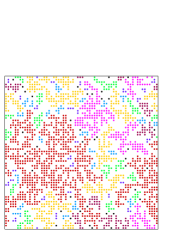
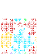
(a) $g=0.4$, $t=859$ (b) $g=0.8$, $t=75$

Figure 1: (Color online) Snapshots of cluster configurations just before the appearance of a spanning cluster: (a) for $g=0.4$ at $t=859$ and (b) for $g=0.8$ at $t=75$ on a $2$D square lattice of size $L=64$. The red color shows the largest cluster and other different colors represent the presence of clusters of different sizes. Periodic boundary condition is applied in both horizontal and vertical directions during cluster growth.

III.1 Cluster morphology and time evolution of the largest cluster

The snapshots of cluster configurations are taken just prior to the appearance of the spanning cluster in the system and are shown in Fig.1 for $g=0.4$ (a), and $g=0.8$ (b) on a $2$D square lattice of size $L=64$. The largest cluster is shown in red and the other smaller clusters of different sizes are depicted in other different colors. At the lower growth probability $g=0.4$, clusters of many different sizes exist along with a large finite cluster. Smaller clusters are found to be enclaved inside the larger clusters. PT occurs in the next step and no significant change in the largest cluster size is expected as the largest cluster in the previous step was about to span the lattice. Such continuous change in the largest cluster size along with enclaved smaller clusters within it are indications of continuous transition Sheinman2015 . On the other hand, as the growth probability is taken to be high $g=0.8$, clusters of smaller sizes are merged with the fast growing other finite clusters. As a result, only a few large compact clusters are found to exist beside the newly planted nucleation centers. Clusters of intermediate sizes are found to be absent. Enclave of smaller clusters by the larger clusters has almost disappeared. As the clusters in cyan and red are merged in the next step and generates a spanning cluster, the PT occurs with a significant change in the size of the largest cluster corresponding to a jump in the largest cluster size at the time of transition. Appearance of compact large cluster with discontinuous jump in the largest cluster size are indications of a discontinuous transition bfwm031103 .

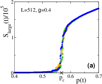
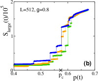
Figure 2: (Color online) Time evolution of the largest cluster $S_{\rm large}(t)$ for a few samples are shown against the area fraction $p(t)$ for $g=0.4$ in (a) and for $g=0.8$ in (b) for a system of size $L=512$.

The time evolution of the size of the largest cluster $S_{\rm large}(t)$ is monitored against the instantaneous area fraction $p(t)$ for three different samples for a given $g$. Their variations are shown in Fig.2(a) for $g=0.4$ and for $g=0.8$ in Fig.2(b) for a system of size $L=512$. The average area fractions corresponding to the thresholds at which PT occur in these systems with given $g$ are marked by the crosses on the respective $p(t)$-axis. Around the respective thresholds, the evolution of the size of the largest clusters for $g=0.4$ and $g=0.8$ are drastically different. For $g=0.4$, the size of the largest cluster in different samples are found to increase almost continuously with the instantaneous area fraction $p(t)$ around the threshold. This indicates a continuous PT to occur. However, for $g=0.8$, $S_{\rm large}$ grows with discontinuous jumps at the threshold with the largest jump of the order of $10^{5}\gg L$. The effect would be more prominent with higher values of $g$. This is another indication of a discontinuous PT. It is then intriguing to study the model with varying the growth probability $g$ and characterize the nature of transitions at different regimes of $g$.

III.2 Fluctuation in order parameter

The dynamical order parameter $P_{\infty}(t)$, the probability to find a lattice site in the spanning cluster, is defined as

$$P_{\infty}(t)=\frac{S_{\rm max}(t)}{L^{2}}$$ (1)

where $S_{\rm max}(t)$ is the size of the spanning cluster at time $t$. The finite size scaling (FSS) form of $P_{\infty}(t)$ is given by

$$P_{\infty}(t)=L^{-\beta/\nu}\widetilde{P}_{\infty}[\{p(t)-p_{c}(g)\}L^{1/\nu}]$$ (2)

where $\widetilde{P}_{\infty}$ is a scaling function, $\beta$ is the order parameter exponent, $\nu$ is the correlation length exponent and $p_{c}(g)$ is the critical area fraction for a given growth probability $g$ at which a spanning cluster connecting the opposite sides of the lattice appears for the first time in the system. Following the formalism of thermal critical phenomena bruce1992 as well as several recent models of percolation Grassberger2011 , the distribution of $P_{\infty}$ is taken as

$$P[P_{\infty}(t)]=L^{\beta/\nu}\widetilde{P}[P_{\infty}(t)L^{\beta/\nu}]$$ (3)

where $\widetilde{P}$ is a scaling function. With such a scaling form of $P[P_{\infty}(t)]$, one could easily show that

$$\langle P^{2}_{\infty}(t)\rangle\sim L^{-2\beta/\nu}\ \ \ {\rm and}\ \ \ \langle P_{\infty}(t)\rangle^{2}\sim L^{-2\beta/\nu}.$$ (4)

The fluctuation in $P_{\infty}(t)$ at an area fraction $p(t)$ is defined as

$$\chi_{\infty}(t)=\frac{1}{L^{2}}\left[\langle S^{2}_{\rm max}(t)\rangle-{\langle S_{\rm max}(t)\rangle}^{2}\right].$$ (5)

The FSS form of $\chi_{\infty}(t)$ is given by

$$\chi_{\infty}(t)=L^{\gamma/\nu}\widetilde{\chi}[\{p(t)-p_{c}(g)\}L^{1/\nu}]$$ (6)

where $\gamma/\nu=d-2\beta/\nu$ is the ratio of the average cluster size exponent to the correlation length exponent $\nu$, $d$ is space dimension and $\widetilde{\chi}$ is a scaling function.

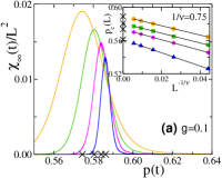
Figure 3: (Color online) Plot of $\chi_{\infty}(t)/L^{2}$ against $p(t)$ for $g=0.1$ (a) and $g=0.8$ (b) for different lattice sizes $L$= $128$ (orange solid line), $256$ (green solid line), $512$ (magenta solid line) and $1024$ (blue solid line). Crosses on the $p(t)$-axis represent the thresholds $p_{c}(L)$. $p_{c}(L)$ is plotted against $L^{-1/\nu}$ taking $1/\nu=0.75$, for $g=0.1(\CIRCLE)$, $0.3(\blacksquare)$, $0.4(\blacklozenge)$, $0.5(\blacktriangle)$ in the inset of (a) and for $g=0.7(\CIRCLE)$, $0.8(\blacksquare)$, $0.9(\blacklozenge)$, $1.0(\blacktriangle)$ in the inset of (b).

In Fig. 3, $\chi_{\infty}(t)/L^{2}$ is plotted against $p(t)$ for different lattice sizes at two extreme values of $g$: $g=0.1$ in Fig.3(a) and $g=0.8$ in Fig.3(b). There are two important features to note. First, each plot has a maximum at a certain value of $p(t)$ for a given $g$ and $L$. The locations of the peaks correspond to the critical thresholds $p_{c}(L)$ (marked by crosses on the $p(t)$ axis) at which a spanning cluster appears for the first time in the system. The critical area fraction $p_{c}(L)$ is expected to scale with the system size $L$ as

$$p_{c}(L)-p_{c}(g)\approx L^{-1/\nu}$$ (7)

where $\nu$ is the correlation length exponent, as it happens in OP stauffer . In the limit $L\rightarrow\infty$, the value of $p_{c}(L)$ becomes $p_{c}(g)$, the percolation threshold of the model for a given $g$. In the insets of respective figures, $p_{c}(L)$ is plotted against $L^{-1/\nu}$ taking $1/\nu=0.75$, that of the OP, for different values of $g$. The scaling form given in Eq.7 is found to be well satisfied for $g\leq 0.5$ with $1/\nu=0.75$, inset of Fig.3(a). For $g\leq 0.5$, the linear extrapolation of the plots of different $g$ intersect the $p_{c}(L)$ axis at different $p_{c}(g)$ values. Whereas for $g\geq 0.8$, the data do not obey Eq.7 and no definite $p_{c}(g)$ is found to exist in the $L\to\infty$ limit. Such deviation from the scaling form given in Eq.7 is found to occur for the systems those are grown with $g>0.5$ too.

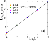
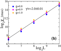
Figure 4: (Color online) Plot of $\chi_{\infty}(\rm max)$ against $L$ for $g\leq 0.5$ is given in (a) and for $g\geq 0.8$ is given in (b). The straight lines of slope $\gamma/\nu=1.79$ and $\gamma/\nu=2.0$ in (a) and (b) respectively are guide to eye.

Second, the peak values of $\chi_{\infty}(t)/L^{2}$ are decreasing with increasing $L$ for $g=0.1$ as in continuous transitions whereas they remain constant with $L$ for $g=0.8$ as in discontinuous transitions PhysRevLett.105.035701 . In order to extract the exponent $\gamma/\nu$ for a system with a given value of $g$, the peak values of the fluctuation $\chi_{\infty}(\rm max)$ are plotted against $L$ for $g\leq 0.5$ in Fig.4(a) and for $g\geq 0.8$ in Fig.4(b) in double logarithmic scale. The magnitudes of $\chi_{\infty}(\rm max)$ are found to be independent of $g$ at a given $L$ for $g\leq 0.5$ whereas they increase with $g$ at a given $L$ for $g\geq 0.8$. As per the scaling relation Eq.6, a power law scaling $\chi_{\infty}(\rm max)\sim L^{\gamma/\nu}$ is expected to follow at the threshold. The exponent $\gamma/\nu$ is determined by linear least square fit through the data points. For $g\leq 0.5$, it is found to be $\gamma/\nu=1.79\pm 0.01$ whereas for $g\geq 0.8$, it is found to be $\gamma/\nu=2.0\pm 0.01$. The solid straight lines with desire slopes in Fig.4(a) and (b) are guide to eye. It is important to note that the value of $\gamma/\nu$ for $g\leq 0.5$ is that of the OP ($43/24$) which indicates continuous transitions whereas for $g\geq 0.8$ it is that of the space dimension which indicates discontinuous transitions. For $0.5<g<0.8$, the exponent $\gamma/\nu$ is found to change continuously from $1.79$ to $2.0$ indicating a region of crossover. The values of $\gamma/\nu$ for different values of $g$ are also verified by estimating the average cluster size of all the finite clusters (excluding the spanning cluster) at their respective percolation thresholds. However, there are evidences in some other percolation models such as $k$-core percolation PhysRevE.94.062307 that the scaling behavior of order parameter fluctuation and that of the average cluster size are not identical.

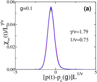
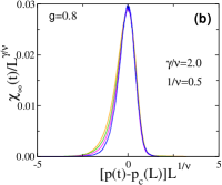
Figure 5: (Color online) Plot of $\chi_{\infty}(t)/L^{\gamma/\nu}$ against the scaled variable $[{p(t)-p_{c}}L^{1/\nu}]$ for $g=0.1$ (a) and for $g=0.8$ (b) respectively.

The FSS form of $\chi_{\infty}(t)$ is verified plotting the scaled fluctuation $\chi_{\infty}(t)/L^{\gamma/\nu}$ against the scaled variable $[p(t)-p_{c}(g)]L^{1/\nu}$ for $g=0.1$ in Fig.5(a). A good collapse of data is obtained for $\gamma/\nu=1.79$ and $1/\nu=0.75$ as those of OP. Whereas, for $g=0.8$, a partial collapse is obtained for the plots of $\chi_{\infty}(t)/L^{\gamma/\nu}$ against the scaled variable $[p(t)-p_{c}(L)]L^{1/\nu}$, as no $p_{c}(g)$ is available, taking $\gamma/\nu=2.0$ and tuning the value of $1/\nu$ to $0.5$ as shown in Fig.5(b). The collapse of the peak values confirms the values of the scaling exponent $\gamma/\nu$ as $1.79$ for $g\leq 0.5$ and $2.0$ for $g\geq 0.8$. Following the scaling relation $\gamma/\nu=d-2\beta/\nu$, the exponent $\beta/\nu$ should be $0.105$ as that of OP for $g\leq 0.5$ and zero as that of a discontinuous PT for $g\geq 0.8$.

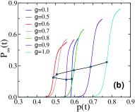
Figure 6: (Color online) (a) Plot of $p_{c}(L)$ against $g$. (b) Plot of $P_{\infty}(t)$ against $p(t)$ for different values of $g$ for $L=1024$.

III.3 Phase diagram

A phase diagram separating the percolating and non-percolating regions is obtained by plotting the variation of $p_{c}(L)$ against $g$ for a system of size $L=1024$ in Fig.6(a). It is interesting to note that the critical area fraction has a minimum at a growth probability little above the threshold of OP, $p_{c}$(OP)$\approx 0.5927$ and it is as low as $\approx 0.45$. It is obvious that area fraction would be $\approx 0.6$ at the criticality when $g=0$. If $g$ is finite but small, growth of small clusters will stop mostly because of less growth probability beside rarely merging with another small cluster or a newly added nucleation center. A large number of smaller clusters will be there in the system before transition and merging of such small cluster will lead to a spanning cluster which will have many voids in it. As a result, the area fraction will be less. Such an effect will be more predominant when $g$ is around the percolation threshold of OP as at this growth probability large fractal clusters will be grown. PT occurs due to merging of such large fractal clusters which will contain maximum void space in it. Hence, the area fraction is expected to be the lowest. Beyond, such growth probability, compact clusters start appearing which will occupy most of the space at the time of transition. Area fraction will increase almost linearly with $g$ in this regime. Such variation of $p_{c}$ is also observed in a percolation model with repulsive or attractive rule in site occupation refId0 .

The phase diagram is then complemented by the variations of $P_{\infty}(t)$ against $p(t)$ for various values of $g$ which are shown in Fig.6(b). Not only the the critical threshold decreases with increasing $g$ and takes a turn at $g\approx 0.65$ but also the transitions become more and more sharper as $g$ increases beyond $g\approx 0.65$. It is also interesting to note that values $P_{\infty}(t)$ at $p_{c}$ also increases with increasing $g$ even when the critical area fraction ($p_{c}$) is decreasing. Therefore the spanning cluster mass is always increases with the growth probability $g$.

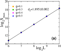
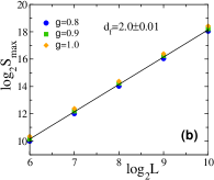
Figure 7: (Color online) Plot of $S_{\rm max}$ against lattice sizes $L$ at their respective thresholds for $g\leq 0.5$ in (a) and for $g\geq 0.8$ in (b). The solid straight line of slope $1.896$ in (a) and that of slope $2.0$ in (b) are guide to eye.

III.4 Dimension of spanning cluster

For system size $L\ll\xi$, the size of the spanning cluster $S_{\rm max}$ at the criticality varies with the system size $L$ as

$$S_{\rm max}\approx L^{d_{f}}$$ (8)

where $d_{f}$ is the fractal dimension of the spanning cluster. Since the clusters are grown here applying PBC, the horizontal and vertical extensions of the largest cluster are stored. If either the horizontal or the vertical extension of the largest cluster is found to be greater than or equal to $L$, it is identified as a spanning cluster. The value of $S_{\rm max}$ are noted at the respective thresholds for several lattice sizes $L$ for a given $g$. For a continuous PT, the spanning cluster is a random object with all possible sizes of holes in it and is expected to be fractal whereas in the case of a discontinuous transition it becomes a compact cluster. The values of $S_{\rm max}$ are plotted against $L$ in double logarithmic scale for the different values of $g\leq 0.5$ in Fig. 7(a) and for $g\geq 0.8$ in Fig. 7(b). For $g\leq 0.5$, $S_{\rm max}$ scales with $L$ as a power law with $d_{f}=1.895\pm 0.002$ almost that of OP ($91/48$). On the other hand, for $g\geq 0.8$, $S_{\rm max}$ scales with $L$ as a power law with $d_{f}=2.0\pm 0.01$ as that of space dimension $d$. The solid lines with desire slopes $1.896$ and $2.0$ in Fig.7(a) and (b) respectively are guide to eye. Thus for $g\leq 0.5$, the spanning cluster is found to be fractal as in OP whereas for $g\geq 0.8$ they appear to be compact as expected in a discontinuous transition. As a result, there would be enclaves in spanning clusters for $g\leq 0.5$ whereas such enclaves would be absent in the spanning clusters for $g\geq 0.8$ as it is evident in the cluster morphology shown in Fig. 1. Such presence or absence of enclaves in the spanning cluster determines whether it would be fractal or compact which essentially determines the nature of the transition as continuous or discontinuous Sheinman2015 ; PhysRevLett.106.095703 . In the regime $0.5<g<0.8$ the dimension of spanning cluster $d_{f}$ changes continuously from $d_{f}=1.895$ to $d_{f}=d=2.0$.

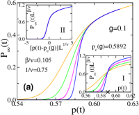
Figure 8: (Color online) Plot of $P_{\infty}(t)$ against $p(t)$ for $g=0.1$ (a) and $g=0.8$ (b). In the inset-I of (a) for $g=0.1$, $P_{\infty}(t)L^{\beta/\nu}$ is plotted against $p(t)$ taking $\beta/\nu=0.105$ and in the inset-II of (a) it is plotted against the scaled variable $[p(t)-p_{c}(g)]L^{1/\nu}$ taking $1/\nu=0.75$. In the inset of (b) for $g=0.8$, $P_{\infty}(t)L^{\beta/\nu}$ is plotted against $[p(t)-p_{c}(L)]L^{1/\nu}$ taking $\beta/\nu=0$ and $1/\nu=0.5$. Same set of color symbols of Fig. 3 for different system sizes are used

III.5 FSS of $P_{\infty}(t)$

The FSS form of $P_{\infty}(t)$ given in Eq.2 as $L^{-\beta/\nu}\widetilde{P}_{\infty}[\{p(t)-p_{c}(g)\}L^{1/\nu}]$ should scales with the system size $L$ as $P_{\infty}(t)\sim L^{-\beta/\nu}$ at the criticality where $\beta/\nu=d-d_{f}$. As the value of $d_{f}$ is found to be $1.895$ for $g\leq 0.5$ and $2.0$ for $g\geq 0.8$, it is expected that the order parameter exponent $\beta/\nu$ should be $0.105$ as that OP ($5/48$) for $g\leq 0.5$ and zero for $g\geq 0.8$ leading to discontinuous jump. A continuous variation in $\beta/\nu$ is expected in the regime $0.5<g<0.8$. Variation of $P_{\infty}(t)$ is plotted against $p(t)$ for different lattice sizes for $g=0.1$ in Fig. 8(a) and for $g=0.8$ in Fig. 8(b). As the system size $L$ increases, $P_{\infty}(t)$ becomes sharper and sharper for both $g=0.1$ and $g=0.8$. However, the plots of $P_{\infty}(t)L^{\beta/\nu}$ cross at a particular value of $p(t)$ corresponding to the critical threshold $p_{c}(g)$ taking $\beta/\nu=0.105$ for $g=0.1$ as shown in inset-I of Fig. 8(a). As $\beta/\nu=0$ for $g=0.8$, by no means they could make cross at a definite $p(t)$. However, for $g=0.1$, after re-scaling the $P_{\infty}(t)$ axis if the $p(t)$ axis is re-scaled as $[p(t)-p_{c}(g)]L^{1/\nu}$ taking $1/\nu=0.75$ a complete collapse of data occurs as shown in inset-II of Fig. 8(a). Whereas, for $g=0.8$, collapse of $P_{\infty}(t)$ plots are obtained by re-scaling only the $p(t)$ axis as $[p(t)-p_{c}(L)]L^{1/\nu}$ taking $1/\nu=0.5$ as shown in the inset of Fig. 8(b). Such collapse of data not only confirms the validity of the scaling forms assumed but also confirms the values of the scaling exponents obtained. The observations at $g=0.1$ are found to be the same for all $g\leq 0.5$ and those are at $g=0.8$ are same for $g\geq 0.8$. Though discontinuous jump in the order parameter is also observed in SFM, the PT is characterized as continuous Chakraborty2014 . On the other hand, in GCM, discontinuous transition is found to occur only in the vanishingly small fixed initial seed concentration Tsakiris2011 but for intermediate seed concentrations the transitions are found to continuous that belong to OP universality class argtouchstop ; PhysRevE.87.022115 . For $0.5<g<0.8$, collapse of data is observed for continuously varied exponents that depend on $g$ as also seen in Ref.PhysRevE.88.042122 . The variations of the critical exponents $\gamma/\nu$, $\beta/\nu$ and fractal dimension $d_{f}$ with the growth probability $g$ are presented in Fig. 9. The values of the critical exponents clearly distinguishes the discontinuous transitions for $g\geq 0.8$ from the continuous transitions for $g\leq 0.5$.

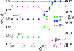
Figure 9: (Color online) Values of the critical exponents against the growth probability $g$ are shown for $\gamma/\nu$ (green circle), $\beta/\nu$ (magenta triangle), and fractal dimension $d_{f}$ (blue square).

III.6 Binder cumulant

The evidences presented above indicate a continuous transition for $g\leq 0.5$ and a discontinuous transition for $g\geq 0.8$. In order to confirm the order of transition in different regimes of the growth probability $g$, a dynamical Binder cumulant $B_{L}(t)$ PhysRevB.34.1841 ; 1stfssbinder , the fourth moment of $S_{\rm max}(t)$, is studied as function of area fraction $p(t)$. The dynamical Binder cumulant $B_{L}(t)$ is defined as

$$B_{L}(t)=\frac{3}{2}\bigg{[}1-\frac{\langle S_{\rm max}^{4}(t)\rangle}{3{\langle S_{\rm max}^{2}(t)\rangle}^{2}}\bigg{]}.$$ (9)

The cumulants when plotted against the area fraction $p(t)$ for different system sizes $L$ are expected to cross each other at a definite $p(t)$ corresponding to the critical threshold of the system for a continuous transition whereas no such crossing is expected to occur in the case of a discontinuous transition Roy010101 . Though the cumulant has some unusual behavior TSAI1998 ; botet , it is rarely used in the study of recent models of percolation. The values of $B_{L}(t)$ are plotted against $p(t)$ for different system sizes $L$ in Fig. 10(a) for $g=0.1$ and in Fig. 10(b) for $g=0.8$. For $g=0.1$, the plots of $B_{L}(t)$ cross at a particular $p(t)$ corresponding to $p_{c}(g)$, marked by a cross on the $p(t)$-axis whereas for $g=0.8$ no such crossing of $B_{L}(t)$ is observed for different values of $L$. The value of the Binder cumulant at the critical threshold $B_{L}(p_{c})$ is found to be $0.945$ as shown by a dotted line in Fig.10(a) for $g=0.1$ and remains close to this for other values of $g\leq 0.5$. It is verified that the value of $B_{L}(p_{c})$ is same as that of ordinary site percolation though it reported little less for the bond percolation PhysRevE.71.016120 .

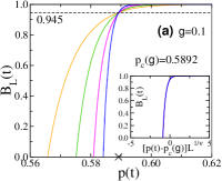
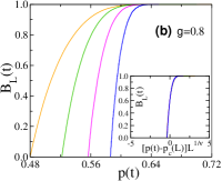
Figure 10: (Color online) Plot of Binder cumulant $B_{L}(t)$ against $p(t)$ for the different lattice sizes in (a) for $g=0.1$ and in (b) for $g=0.8$. The same color symbols of Fig. 3 for different system sizes are used. Plot of $B_{L}(t)$ against the scaled variable $[p(t)-p_{c}]L^{1/\nu}$ are given in the respective insets taking appropriate values of $1/\nu$.

The FSS form of $B_{L}(t)$ is given by

$$B_{L}(t)=\widetilde{B}[(p(t)-p_{c})L^{1/\nu}]$$ (10)

where $\widetilde{B}$ is a universal scaling function. The FSS form is verified by obtaining a collapse of the plots of $B_{L}(t)$ against the scaled variable $[p(t)-p_{c}(g)]L^{1/\nu}$ taking $1/\nu=0.75$ for $g=0.1$. For $g=0.8$, however, such a collapse is obtained when the cumulants are plotted against $[p(t)-p_{c}(L)]L^{1/\nu}$ taking $1/\nu=0.5$. The data collapse is shown in the insets of the respective plots. Such scaling behavior of $B_{L}(t)$ for $g=0.1$ is found to occur for the whole range of $g\leq 0.5$ and that of $g=0.8$ is found to occur for $g\geq 0.8$. Once again, Binder cumulant provides a strong evidence that the dynamical transition is continuous for $g\leq 0.5$ whereas it is discontinuous for $g\geq 0.8$. For $0.5<g<0.8$, a region of crossover, the cumulants do not cross at a particular value of $p(t)$ rather they cross each other over a range of $p(t)$ values but do collapse when plotted against the scaled variable $[p(t)-p_{c}(L)]L^{1/\nu}$ for the respective value of $1/\nu$ for a given value of $g$.

III.7 Cluster size and order parameter distributions

Power law distribution of cluster sizes at the critical threshold is an essential criteria in a second-order continuous phase transition. Following OP, a dynamical cluster size distribution $n_{s}(t)$, the number of clusters of size $s$ per lattice site at time $t$, is assumed to be

$$n_{s}(t)=s^{-\tau}{\sf f}[(p(t)-p_{c})s^{\sigma}]$$ (11)

where $\tau$ and $\sigma$ are two exponents and ${\sf f}$ is a universal scaling function. For OP, an equilibrium percolation model, the exponents are $\tau=187/91$ and $\sigma=36/91$ stauffer . The distribution at the percolation threshold $n_{s}(p_{c})$ is expected to scale as $\approx s^{-\tau}$. The cluster size distributions $n_{s}(p_{c})$ are determined taking $p_{c}(g)$ as threshold for $g\leq 0.5$ and taking $p_{c}(L)$ as threshold for $g\geq 0.8$ for a system of size $L=1024$. The data obtained are binned of varying widths and finally normalized by the respective bin widths. In Fig. 11(a), the distributions $n_{s}(p_{c})$ are plotted against $s$ in double logarithmic scale for $g\leq 0.5$ ($0.4$ (green) and $0.5$ (magenta)) and for $g\geq 0.8$ ($0.9$ (orange) and $1.0$ (blue)) for $L=1024$. It is clearly evident that the distributions for $g\leq 0.5$ describes a power law behavior whereas for $g\geq 0.8$ the distributions develop curvature and deviate from power law scaling. In the inset, the measured exponent $\tau_{s}=\partial\log_{10}n_{s}(p_{c})/\partial\log_{10}s$ is plotted against $\log_{10}s$. The value of $\tau_{s}$ remains constant to $\approx 2.055$ as that of OP over a wide range of $s$ for $g\leq 0.5$ whereas $\tau_{s}$ varies with $s$ for $g\geq 0.8$ indicating no definite value of $\tau$. The existence of a crossover from continuous transition of OP type to a discontinuous percolation transition is further confirmed by the value of $\tau$ in the different regimes of the growth probability $g$. This is in contrary to the observations in SFM Chakraborty2014 or cluster merging model Cho2016 where a power law distribution of clusters size is found to occur beside discontinuous transition.

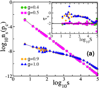
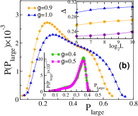
Figure 11: (Color online) (a) Plot of $n_{s}(p_{c})$ against $s$ for different values of $g=0.4[\CIRCLE]$ (green), $0.5[\blacksquare]$ (magenta), $0.9[\blacklozenge]$ (orange) and $1.0[\blacktriangle]$ (blue) for $L=1024$. Variation of the local slope $\tau_{s}$ $vs$ $s$ for the same set of $g$ values are shown in the inset of (a). (b) Plot of $P(P_{\rm large})$ against $P_{\rm large}$ for the corresponding systems in (a). For $g=0.4$ and $0.5$, plots are given as an inner plot using different scale. In the inset at top right corner of (b), plot of $\Delta$ against $L$ for $g=0.8[\CIRCLE]$ (violet), $0.9[\blacksquare]$ (orange) and $1.0[\blacktriangle]$ (blue).

Beside the cluster size distribution, distribution of order parameter is also studied for different values of $g$ as usually it is studied in thermal phase transitions bruce1992 where a bimodal distribution of order parameter is expected in a discontinuous transition whereas single peaked distribution is obtained in a continuous transition. An ensemble of largest clusters on different configurations are collected at the percolation threshold of a given $g$ and the values of the order parameter $P_{\rm large}=S_{\rm large}/L^{2}$ are estimated. A probability distribution $P(P_{\rm large})$ is then defined as

$$P(P_{\rm large})\sim L^{\beta/\nu}\widetilde{P}[P_{\rm large}L^{\beta/\nu}]$$ (12)

where $\widetilde{P}$ is a scaling function. Bimodal nature of $\widetilde{P}$ is found to be a powerful tool to distinguish discontinuous transitions from continuous transitions in some of the recent percolation models Grassberger2011 ; Manna20122833 ; Tian2012286 ; Roy010101 . The distributions of $P(P_{\rm large})$s are plotted in Fig. 11(b) for different values of $g$. For $g\geq 0.8$, instead of sharp bimodal distributions, broad distributions with two weak peaks are obtained. No FSS of the distributions is found as given Eq.12 but the width of the distribution $\Delta=2[\langle P_{\rm large}^{2}\rangle-\langle P_{\rm large}\rangle^{2}]^{1/2}$ for a given $g$ is found to increase with the system size $L$, shown in the inset of Fig. 11(b), as a signature of discontinuous transition. For a given $L$, the width of the distributions $\Delta$ is also found to increase with $g$. However, the distributions $P(P_{\rm large})$ for $g\leq 0.5$ are found to be single humped and follow the scaling form given in Eq.12 as shown in the other inset. The width of the distributions for a given $g\leq 0.5$ is found to decrease with $L$. The model, thus, exhibits characteristic properties of discontinuous transition for $g\geq 0.8$ and those of continuous transition for $g\leq 0.5$.

IV Conclusion

In a dynamical model of percolation with random growth of clusters from continuously implanted nucleation centers through out the growth process with touch and stop rule, a crossover from continuous to discontinuous PT is observed as the growth probability $g$ tuned from $0$ to $1$. For $g\leq 0.5$, the order parameter continuously goes to zero and the geometrical quantities follow the usual FSS at the critical threshold with the critical exponents that of OP. The cluster size distribution is found to be scale free and a single humped distribution of order parameter occurred in this regime of $g$. On the other hand, for $g\geq 0.8$, the PT occurs with a discontinuous jump at the threshold, the order parameter fluctuation per lattice site becomes independent of system size, the spanning cluster becomes compact with fractal dimension $d_{f}=2$ as that of discontinuous transitions. No scale free distribution is found for the cluster sizes and the order parameter distribution is weakly double humped broad distribution of increasing width with the system size. The order of transitions in different regimes of $g$ are further confirmed by the estimates of Binder cumulant. The intermediate regime of growth probability $0.5<g<0.8$ remains a region of crossover without a definite tricritical point.

References

- (1) N. Araújo, P. Grassberger, B. Kahng, K. Schrenk, and R. Ziff, The European Physical Journal Special Topics 223, 2307 (2014).
- (2) A. Saberi, Physics Reports 578, 1 (2015).
- (3) S. Boccaletti et al., Physics Reports 660, 1 (2016).
- (4) D. S. Callaway, J. E. Hopcroft, J. M. Kleinberg, M. E. J. Newman, and S. H. Strogatz, Phys. Rev. E 64, 041902 (2001).
- (5) P. S. Dodds and D. J. Watts, Phys. Rev. Lett. 92, 218701 (2004).
- (6) H.-K. Janssen, M. Müller, and O. Stenull, Phys. Rev. E 70, 026114 (2004).
- (7) J. M. Schwarz, A. J. Liu, and L. Q. Chayes, EPL (Europhysics Letters) 73, 560 (2006).
- (8) X. Yuan, Y. Dai, H. E. Stanley, and S. Havlin, Phys. Rev. E 93, 062302 (2016).
- (9) D. Achlioptas, R. M. D’Souza, and J. Spencer, Science 323, 1453 (2009).
- (10) R. M. Ziff, Phys. Rev. Lett. 103, 045701 (2009).
- (11) Y. Cho, S. Hwang, H. Herrmann, and B. Kahng, Science 339, 1185 (2013).
- (12) S. V. Buldyrev, R. Parshani, G. Paul, H. E. Stanley, and S. Havlin, Nature 464, 1025 (2010).
- (13) D. Zhou, A. Bashan, R. Cohen, Y. Berezin, N. Shnerb, and S. Havlin, Phys. Rev. E 90, 012803 (2014).
- (14) F. Radicchi, Nature Physics 11, 597 (2015).
- (15) G. Bizhani, P. Grassberger, and M. Paczuski, Phys. Rev. E 84, 066111 (2011).
- (16) C. Christensen, G. Bizhani, S.-W. Son, M. Paczuski, and P. Grassberger, EPL 97 (2012).
- (17) S. Boettcher, V. Singh, and R. Ziff, Nature Communications 3 (2012).
- (18) K. J. Schrenk, M. R. Hilário, V. Sidoravicius, N. A. M. Araújo, H. J. Herrmann, M. Thielmann, and A. Teixeira, Phys. Rev. Lett. 116, 055701 (2016).
- (19) P. Grassberger, Phys. Rev. E 95, 010103 (2017).
- (20) B. Roy and S. B. Santra, Phys. Rev. E 95, 010101 (2017).
- (21) D. Stauffer and A. Aharony, Introduction to Percolation Theory, Taylor and Francis, London, 1994.
- (22) A. Bunde and S. Havlin, Fractals and Disordered Systems, Springer-Verlag, Berlin, 1991.
- (23) Y. S. Cho, B. Kahng, and D. Kim, Phys. Rev. E 81, 030103 (2010).
- (24) N. A. M. Araújo and H. J. Herrmann, Phys. Rev. Lett. 105, 035701 (2010).
- (25) H.-K. Janssen and O. Stenull, EPL 113, 26005 (2016).
- (26) P. Shu, L. Gao, P. Zhao, W. Wang, and H. Stanley, Scientific Reports 7 (2017).
- (27) N. A. M. Araújo, J. S. Andrade, R. M. Ziff, and H. J. Herrmann, Phys. Rev. Lett. 106, 095703 (2011).
- (28) L. Cao and J. M. Schwarz, Phys. Rev. E 86, 061131 (2012).
- (29) K. Chung, Y. Baek, M. Ha, and H. Jeong, Phys. Rev. E 93, 052304 (2016).
- (30) F. Radicchi and S. Fortunato, Phys. Rev. E 81, 036110 (2010).
- (31) M. Sheinman, A. Sharma, J. Alvarado, G. H. Koenderink, and F. C. MacKintosh, Phys. Rev. Lett. 114, 098104 (2015).
- (32) Y. S. Cho, J. S. Lee, H. J. Herrmann, and B. Kahng, Phys. Rev. Lett. 116, 025701 (2016).
- (33) R. A. da Costa, S. N. Dorogovtsev, A. V. Goltsev, and J. F. F. Mendes, Phys. Rev. Lett. 105, 255701 (2010).
- (34) O. Riordan and L. Warnke, Science 333, 322 (2011).
- (35) P. Grassberger, C. Christensen, G. Bizhani, S.-W. Son, and M. Paczuski, Phys. Rev. Lett. 106, 225701 (2011).
- (36) N. Bastas, P. Giazitzidis, M. Maragakis, and K. Kosmidis, Physica A: Statistical Mechanics and its Applications 407, 54 (2014).
- (37) A. Chakraborty and S. S. Manna, Phys. Rev. E 89, 032103 (2014).
- (38) N. Tsakiris, M. Maragakis, K. Kosmidis, and P. Argyrakis, The European Physical Journal B 81, 303 (2011).
- (39) N. Tsakiris, M. Maragakis, K. Kosmidis, and P. Argyrakis, Phys. Rev. E 82, 041108 (2010).
- (40) P. L. Leath, Phys. Rev. B 14, 5046 (1976).
- (41) K. J. Schrenk, A. Felder, S. Deflorin, N. A. M. Araújo, R. M. D’Souza, and H. J. Herrmann, Phys. Rev. E 85, 031103 (2012).
- (42) A. D. Bruce and N. B. Wilding, Phys. Rev. Lett. 68, 193 (1992).
- (43) D. Lee, M. Jo, and B. Kahng, Phys. Rev. E 94, 062307 (2016).
- (44) Giazitzidis, Paraskevas, Avramov, Isak, and Argyrakis, Panos, Eur. Phys. J. B 88, 331 (2015).
- (45) O. Melchert, Phys. Rev. E 87, 022115 (2013).
- (46) R. F. S. Andrade and H. J. Herrmann, Phys. Rev. E 88, 042122 (2013).
- (47) M. S. S. Challa, D. P. Landau, and K. Binder, Phys. Rev. B 34, 1841 (1986).
- (48) K. Binder and D. P. Landau, Phys. Rev. B 30, 1477 (1984).
- (49) S.-H. Tsai and S. R. Salinas, Brazilian Journal of Physics 28, 58 (1998).
- (50) A. Hasmy, R. Paredes, O. Sonneville-Aubrun, B. Cabane, and R. Botet, Phys. Rev. Lett. 82, 3368 (1999).
- (51) E. Machado, G. M. Buendía, P. A. Rikvold, and R. M. Ziff, Phys. Rev. E 71, 016120 (2005).
- (52) S. Manna, Physica A: Statistical Mechanics and its Applications 391, 2833 (2012).
- (53) L. Tian and D.-N. Shi, Physics Letters A 376, 286 (2012).