Matched shadow processing

Abstract

Traditional matched field processing is based on the comparison of the complex amplitudes of the measured and calculated wave fields at the aperture of the receiving antenna. This paper considers an alternative approach based on comparing the intensity distributions of these fields in the "depth – arrival angle" plane. To construct these intensities, the formalism of coherent states borrowed from quantum mechanics is used. The main advantage of the approach under consideration is its low sensitivity to the inevitable inaccuracy of an environmental model used in calculation.

1 Introduction

The applicability region of the traditional matched field processing (MFP) [1, 2], based on the comparison of the complex amplitudes of the measured and calculated sound fields, is substantially limited by the fact that the complex field amplitude – especially at high frequencies – is very sensitive to variations in the environmental parameters. Therefore, the inevitable inaccuracies of the mathematical model of the environment used in calculations often make the application of MFP impossible [3, 4, 5].

This paper discusses an alternative approach for comparing measured and calculated fields. Here we use the field expansion in coherent states [6, 7]. The intensity (amplitude squared) of the coherent state can be interpreted as a contribution to the total energy of the sound field from waves arriving at a given depth interval at grazing angles from a given angular interval. The set of amplitudes squared of all coherent states gives the distribution of the sound field intensity in the phase plane "depth – arrival angle". In quantum mechanics, an analogous characteristic of a wave function is called the Husimi distribution [8, 9].

Our idea is that instead of comparing the complex amplitudes of the measured and calculated fields, we can compare the intensity distributions of these fields in the phase space, which are less sensitive to variations in the environmental parameters. We divide the phase space into two zones: an insonified zone in which the field intensity is relatively large, and a shadow zone where the intensity is close to zero. The parameter by which the fields are compared is the ratio of the integral intensities in the insonified zone and in the shadow zone. In fact, our method is based on comparing the areas occupied by the shadow zones of the measured and calculated fields (at the same time, the areas occupied by the insonified zones are also compared). Therefore, we call this approach the matched shadow processing (MSP).

The proposed approach is motivated by the results of the recent work [7], where the expansion in coherent states is used to isolate the components of the sound field which are low sensitive to sound speed fluctuations.

In Sec. 2, a definition of the field intensity distribution in phase plane is given and an example is presented of calculating such a distribution for an idealized model of a waveguide in a shallow sea. The similarity coefficient of the measured and calculated fields, based on a comparison of the distributions of their intensities, is introduced in Sec. 3. In Secs. 4 and 5 it is shown that this coefficient is much less sensitive to variations in the environmental parameters and source position than the similarity coefficient used in the traditional MFP.

2 Field intensity distribution in the phase plane

Consider a CW sound field excited by a point source at frequency $f$ in a two-dimensional underwater waveguide with the sound speed field $c\left(r,z\right)$, where $r$ is the range and $z$ is the depth. The refractive index is $n\left(r,z\right)=c_{0}/c(r,z)$, where $c_{0}$ is the reference sound speed satisfying condition $\left|c\left(r,z\right)-c_{0}\right|\ll c_{0}$.

In the scope of the Hamiltonian formalism the ray path at range $r$ is determined by its vertical coordinate $z$ and momentum $p=n\left(r,z\right)\sin\chi$, where $\chi$ is the ray grazing angle. It is assumed that the sound field is excited by a point source set at point $\left(0,z_{s}\right)$. Different rays escape this points with different starting momenta $p_{0}$. Momenta and depths of rays at the observation range $r$ are described by functions $p\left(p_{0}\right)$ and $z\left(p_{0}\right)$, respectively. In phase plane (momentum $P$ – depth $Z$), the arrivals of rays form a curve, which we call the ray line. It is defined by the relations $P=p\left(p_{0}\right)$ and $Z=z\left(p_{0}\right)$.

The ray line establishes a correspondence between the depths and the arrival angles of the rays. Changing the environmental parameters or the source position is manifested in the change of this line. Therefore, the comparison of the ray lines of the measured and calculated fields can be used in solving inverse problems. Although the uncertainty principle does not allow the accurate reconstruction of the ray line, one can restore a fuzzy version of this line. In Ref. [7] it is shown that this can be done using the field expansion in coherent states.

The coherent state associated with the point of the phase plane $\mu=\left(P,Z\right)$ is given by the function [6, 7, 10]

$$Y\left(z;P,Z\right)=\frac{1}{\sqrt{\Delta_{z}}}\exp\left[ikP\left(z-Z\right)-\frac{\pi\left(z-Z\right)^{2}}{2\Delta_{z}^{2}}\right],$$ (1)

where $k=2\pi f/c_{0}$, $\Delta_{z}$ is the width of the coherent state along the $z$-axis. It describes waves arriving at depths close to $Z$ at grazing angles close to $\chi=\arctan P$. The scalar product of coherent states associated with points $\mu_{1}=\left(P_{1},Z_{1}\right)$ and $\mu_{2}=\left(P_{2},Z_{2}\right)$ is

$$\left|\int dz~{}Y_{\mu_{1}}\left(z\right)Y_{\mu_{2}}^{\ast}\left(z\right)\right|=\frac{1}{\sqrt{2}\Delta_{z}}\exp\left(-\frac{\pi}{2}d\left(\mu_{1},\mu_{2}\right)\right),$$

where the asterisk denotes complex conjugation,

$$d\left(\mu_{1},\mu_{2}\right)=\frac{\left(P_{2}-P_{1}\right)^{2}}{\Delta_{p}^{2}}+\frac{\left(Z_{2}-Z_{1}\right)^{2}}{\Delta_{z}^{2}},$$

$\Delta_{p}=\lambda/(2\Delta_{z})$, $\lambda=2\pi/k$ is the wavelength. Function $d\left(\mu_{1},\mu_{2}\right)$ can be interpreted as a dimensionless distance between the points of the phase plane $\mu_{1}$ and $\mu_{2}$. The coherent states associated with these points will be assumed to be close for $d<1$ and different for $d>1$.

Let us define the amplitude of the coherent state as

$$a_{\mu}=\int dz~{}u\left(z\right)Y_{\mu}^{\ast}\left(z\right).$$ (2)

The dependence $\left|a_{\mu}\right|^{2}$ on $\mu$ will be interpreted as the distribution of the intensity of the sound field in the phase plane $P-Z$. In quantum mechanics $\left|a_{\mu}\right|^{2}$ is called the Husimi distribution. It is the Wigner function of the wave field smoothed over the elementary phase plane cell of size $\Delta_{p}\times\Delta_{z}$ [9, 11].  The distribution of intensity $\left|a_{\mu}\right|^{2}$ is localized inside the region, which is formed by points located at distances $d<1$ from the ray line (the distance from a point to a line is the distance to the nearest point of this line). We will call this area the fuzzy ray line.

As an example, let us consider an idealized model of a waveguide in a shallow sea. This is a range-independent waveguide of depth $h$ with a linear sound speed profile. At depths $z=0$ and $z=h$, the sound speed takes values $c_{0}$ and $c$, respectively. The value of $c_{0}$ is taken to be 1.5 km/s.

A waveguide with depth $h=h_{a}$ and $c=c_{a}$, where $h_{a}=$ 190 m and $c_{a}=$ 1.48 km/s, is considered as unperturbed. The sound speed profile in this waveguide is shown in the left panel of Fig. 1. The perturbation is modeled by the deviations of $h$ and $c$ from $h_{a}$ and $c_{a}$, respectively. In addition, by perturbation we also mean changing the source position. As unperturbed values of the source depth and its distance to the antenna, we take $z_{a}=$ 90 m and $r_{a}=$ 2 km, respectively. All calculations are performed at a carrier frequency $f=$ 2000 Hz. The bottom is a liquid half-space with a density of 1400 kg /m³ and a sound speed of 1.6 km / s.

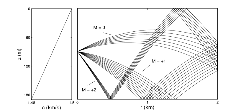
Figure 1: Left panel: unperturbed sound speed profile. Right panel: beams of rays with idenitifiers $M=0$, $M=+1$, and $M=+2$ hitting the antenna.

Using a mode code, the complex amplitude of the wave field is computed at the aperture of receiving antenna, covering the depth interval from $z_{1}=$ 50 m to $z_{2}=$ 150 m and located at different ranges $r$ from the source. When expanding the wave field in coherent states, we take into account only those states that are formed by waves with grazing angles $\left|\chi\right|<18^{\circ}$. Waves with such $\chi$ are formed by modes of the discrete spectrum. This condition means that we consider the intensity $\left|a_{\mu}\right|^{2}$ at the points of the phase plane with $\left|P\right|<\sin 18^{\circ}=0.31$. According to Eqs. (1) and (2), to calculate the amplitude of the state associated with point $\left(P,Z\right)$, one should know the field in the depth interval $Z\pm\Delta_{z}/2$. Therefore, we can find the amplitudes of only those states that are associated with the points of the phase plane at depths $z_{1}+\Delta_{z}/2<Z<z_{2}-\Delta_{z}/2$.

In what follows we consider fields at observation ranges of 1.5 to 2.5 km. At such distances, the field on the antenna is formed by relatively narrow beams of rays, examples of which are shown in the right panel Fig. 2. Each beam includes rays with the same identifier $\pm M$, where $M$ is the number of reflections from the waveguide boundaries, and the + (-) sign means that after leaving the source the first time the ray is reflected from the bottom (surface). At the observation range, the rays of each beam form a segment of the ray line.

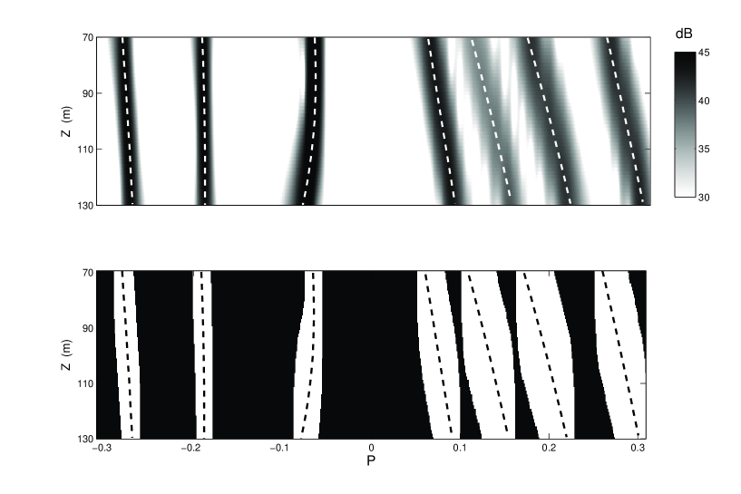
Figure 2: Upper panel: distribution of field intensity $|a_{\mu}|^{2}$ in the phase plane $P-Z$ in the unperturbed waveguide. Lower panel: the insonified zone and the shadow zone are shown in white and black, respectively. The same dashed lines in both panels depict the segments of the ray lines formed by rays with identifiers (from left to right) +3, -2, +1, 0, -1, +2, and -3.

Such segments in the unperturbed waveguide are shown in Fig. 2 by dashed curves. The upper panel of this figure presents the intensity distribution $\left|a_{\mu}\right|^{2}$ at $r=2$ km. Here and below, the projections onto coherent states are calculated with $\Delta_{z}=40$ m. This value of the vertical scale is chosen empirically for a good resolution of fuzzy segments of the ray line.

White areas in the bottom panel of Fig. 2 are formed by points located at distances $d<1$ from the segments of the ray line. These areas form a fuzzy ray line. It represents the insonified zone of the phase plane. We denote this zone $\sigma_{in}$. The remaining part of the phase plane (it is shown in black) is the shadow zone. It will be denoted by $\sigma_{sh}$.

3 Similarity coefficients

Let $u\left(z\right)$ and $\tilde{u}\left(z\right)$ be the complex amplitudes of the sound fields at the receiving antenna in the unperturbed and perturbed waveguide, respectively. The intensities distributions of these fields in the phase plane are $\left|a_{\mu}\right|^{2}$ and $\left|\tilde{a}_{\mu}\right|^{2}$. In the traditional MFP, the similarity of fields $u$ and $\tilde{u}$ is quantitatively characterized by the coefficient [1]

$$K=\frac{\left|\int dz~{}u\left(z\right)\tilde{u}^{\ast}\left(z\right)\right|}{\left(\int dz~{}\left|u\left(z\right)\right|^{2}\right)^{1/2}\left(\int dz~{}\left|\tilde{u}\left(z\right)\right|^{2}\right)^{1/2}}.$$

The main idea of this work is to introduce another similarity coefficient, which is much less sensitive to variations in environmental parameters and source position. This coefficient is $Q=\tilde{q}/q$, where

$$q=\left.\int_{\sigma_{in}}d\mu~{}\left|a_{\mu}\right|^{2}\right/\int_{\sigma_{sh}}d\mu~{}\left|a_{\mu}\right|^{2},\;\tilde{q}=\left.\int_{\sigma_{in}}d\mu~{}\left|\tilde{a}_{\mu}\right|^{2}\right/\int_{\sigma_{sh}}d\mu~{}\left|\tilde{a}_{\mu}\right|^{2}.$$

In these formulas, $q$ is the ratio of the field intensity in the unperturbed waveguide integrated over the insonified zone $\sigma_{in}$ to the intensity integrated over the shadow region $\sigma_{sh}$. The quantity $\tilde{q}$ represents the ratio of the field intensities in the perturbed waveguide integrated over the same zones of the phase plane that were found for the unperturbed waveguide.

Below, with concrete examples, we show that the coefficient $Q$ is indeed much less sensitive to variations in environmental parameters and source position than $K$.

4 Variations in medium parameters and source range

In this section, the sound field $u\left(z\right)$ on the antenna located at range $r=r_{a}$ in the unperturbed waveguide (with $h=h_{a}$ and $c=c_{a}$) is compared with the fields at the same antenna $\tilde{u}\left(z\right)$, calculated for other values of $r$, $h$, and $c$. Calculations performed using the MFP and MSP methods for a fixed source depth $z_{s}=z_{a}$ allow us to find the dependences of the similarity coefficients $K$ and $Q$ on $r$, $h$ and $c$.

Figure 3 shows sections of the uncertainty functions $K(r,h,c)$ (a, c, e) and $Q(r,h,c)$ (b, d, f) by planes $r=r_{a}$ (a,b), $h=h_{a}$ (c,d), and $c=c_{a}$ (e,f). As it is seen, the dependencies of these functions on the arguments $r$, $h$ and $c$ are radically different. Both take their maximum values $K=Q=1$ at the point $\left(r_{a},h_{a},c_{a}\right)$. However, the function $Q(r,h,c)$ gradually decreases with deviation from this point. In contrast, the function $K(r,h,c)$, in addition to the sharp peak at the point $\left(r_{a},h_{a},c_{a}\right)$, has many more local maxima.

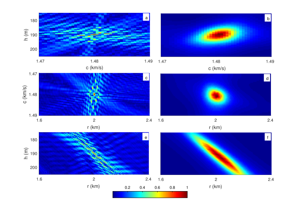
Figure 3: Sections of uncertainty functions $K(r,h,c)$ (left column of plots) and $Q(r,h,c)$ (right column) by planes $r=r_{a}$ (a,b), $h=h_{a}$ (c,d), and $c=c_{a}$ (e,f).

5 Variations of source coordinates

Let us turn to an analysis of the similarity coefficients of the perturbed and unperturbed fields, which are excited by sources located at different distances to the antenna $r_{s}$ and at different depths $z_{s}$. Here we simulate the situation that arises when solving the problem of source localization. Let us assume that the actual values of the distance from the source to the antenna and the source depth are $r_{s}=r_{a}$ and $z_{s}=z_{a}$. The sound field $\tilde{u}(z)$ at the antenna, calculated for a source with such coordinates in, generally speaking, a perturbed waveguide, is regarded as "measured". To restore the source position, the measured field $\tilde{u}(z)$ is compared with the fields $u(z)$ calculated in the unperturbed waveguide for different values of the source coordinates $z_{s}$ and $r_{s}$. The comparison results are expressed by the uncertainty functions $K\left(r_{s},z_{s}\right)$ and $Q\left(r_{s},z_{s}\right)$ representing the dependencies of the similarity coefficients $K$ and $Q$ of the measured and calculated fields on the trial source position ($r_{s}$, $z_{s}$).

Figure 4 shows the results of calculating the functions $K\left(r_{s},z_{s}\right)$ (a,c,e) and $Q\left(r_{s},z_{s}\right)$ (b,d, f) in the unperturbed (a,b), slightly perturbed (c,d) and strongly perturbed (e,f) waveguide. The calculations are performed for $r_{s}$ in the interval from 1.5 km to 2.5 km and $z_{s}$ from 20 to 150 m. The $h$ and $c$ parameters of the waveguides used in the simulation are indicated in the plots.

In the unperturbed waveguide, both the functions $K\left(r_{s},z_{s}\right)$ (a) and $Q\left(r_{s},z_{s}\right)$ (b) have peaks with centers at the point $\left(r_{a},z_{a}\right)$. The peak of function $K\left(r_{s},z_{s}\right)$ is very narrow, and in perturbed waveguides (c,e) it splits into sets of local maxima. In contrast, the function $Q\left(r_{s},z_{s}\right)$ has a much wider peak, which, however, remains in the perturbed waveguides (d,f).

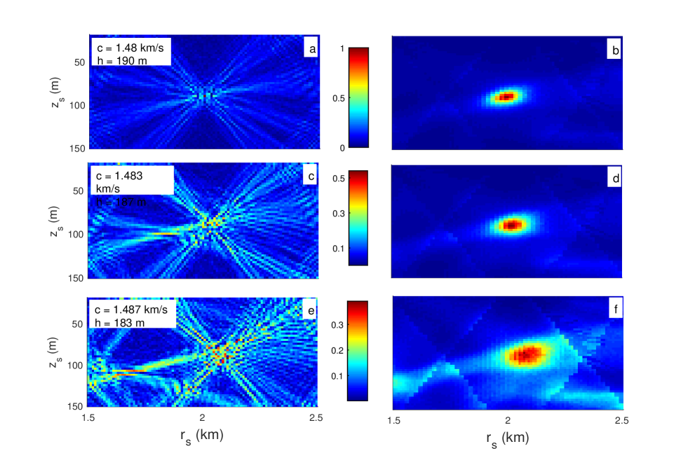
Figure 4: Uncertainty functions $K(r_{s},z_{s})$ (left column of plots) and $Q(r_{s},z_{s})$ (right column) in the unperturbed (a,b), weakly perturbed (c,d), and strongly perturbed waveguide (e,f).

The abrupt changes in the coefficient $Q$ in Figs. 3b, d, and f, which are observed near some inclined lines, can be explained as follows. The intersection of these lines by the point $\left(r_{s},z_{s}\right)$ causes a change in the set of identifiers $\pm M$ of rays arriving at the antenna at grazing angles $\left|\chi\right|<18^{\circ}$ used in constructing the zones $\sigma_{in}$ and $\sigma_{sh}$. This leads to a change in these zones and, accordingly, to a jump in $Q$.

The simulation results suggest that based on MSP, a robust source localization algorithm can be created that is applicable in conditions of inaccurate knowledge of environmental parameters.

6 Conclusion

The main idea of the work is that, under conditions of inaccurate knowledge of the environmental model, instead of the coefficient $K$ quantitatively characterizing the proximity of the complex amplitudes of the calculated and measured fields, the use of a coefficient $Q$ characterizing the proximity of the intensity distributions of these fields in the phase space, can be more effective. With the example of highly idealized waveguide model it is shown that the coefficient $Q$, indeed, much weaker than $K$ varies with variations in the environmental parameters and source position.

In Ref. [7] some considerations are given explaining the stability of field components formed by coherent states associated with small areas of the phase space. These considerations can be used to justify the stability of the intensity distribution $\left|a_{\mu}\right|^{2}$ in phase space.

Another argument is that the ray line in the neighborhood of which the insonified zone is localized is independent of frequency and it much less "feels" the variations in the medium parameters than the complex field amplitude. Therefore, it is natural to expect that the coefficient $Q$ is not only much more stable than $K$ with respect to the inaccuracy of the medium model, but it can be used at high frequencies, where the applicability of the MFP is usually violated.

It should be understood, however, that the weak sensitivity of the coefficient $Q$ to variations in the medium has its downside. In solving inverse problems, the coefficient $Q$ will react weakly to changes in those unknown quantities that must be recovered. This fact limits the ultimate accuracy of restoring an unknown parameter. An example is the problem of source localization, considered in Sec. 5. The main peak of uncertainty function $K(r_{s},z_{s})$ is substantially narrower than the peak of function $Q(r_{s\text{,}}z_{s})$. Therefore, under conditions of accurate knowledge of the environment model, the traditional MFP method will allow to determine the source position much more accurately. However, with an inaccurate environment model, the MFP fails, while the MSP method allows a rough estimate of the source position.

It is clear that the use of the similarity coefficient $Q$ is just one of the possible variants of comparing expansions in the coherent states of the measured and calculated fields. The analysis of other options is beyond the scope of this paper.

Note that the practical use of the MSP method requires solving a number of issues that were not addressed in this paper. In particular, these are questions of the optimal choice of scale $\Delta_{z}$ and distance $d$, which determines the boundary between the insonified and shadow zones. For the applicability of the method, it is obviously required that the shadow zone occupy a significant part of the phase plane area corresponding to admissible depths and arrival angles. When working with CW signals, this condition can be satisfied only at short enough ranges. Here we did not consider the use of MSP for pulse signals, for which the applicability range of the method may become wider due to the fact that the phase space acquires one more dimension (time).

References

- [1] H.P. Bucker, ‘‘Use of calculated sound fields and matched-field detection to locate sound sources in shallow water,’’ J. Acoust. Soc. Am. 59, 368–373 (1976).
- [2] M.J. Hinich, ‘‘Maximum-likelihood signal processing for a vertical array,’’ J. Acoust. Soc. Am. 54, 499–-453 (1973).
- [3] D.F. Gingras and P. Gerstoft, ‘‘Inversion for geometric and geoacoustic parameters in shallow water: Experimental results,’’ J. Acoust. Soc. Am. 97, 3589–-3598 (1995).
- [4] A.B. Baggeroer,‘‘Why did applications of mfp fail, or did we not understand how to apply mfp?,’’ 1st International Conference and Exhibition on Underwater Acoustics, Corfu Island, Greece: Heraklion (2013).
- [5] F.B. Jensen, W.A. Kuperman, M.B. Porter, and H. Schmidt, Computational Ocean Acoustics (Springer, New York, 2011).
- [6] J.R. Klauder and E.C.G. Sudarshan, Fundamentals of quantum optics (W.A. Benjamin, New York, 1968).
- [7] A.L. Virovlyansky, ‘‘Stable components of sound fields in the ocean,’’ J. Acoust. Soc. Am. 141, 1180–1189 (2017).
- [8] K. Husimi, ‘‘Some formal properties of the density matrix,’’ Proc. Phys. Math. Soc. Jpn. 22, 264–314 (1940).
- [9] D. Makarov, S. Prants, A. Virovlyansky, and G. Zaslavsky, Ray and wave chaos in ocean acoustics (Word Scientific, New Jersey, 2010).
- [10] L.D. Landau and E.M. Lifshitz, Quantum mechanics (Pergamon Press, Oxford, 1977).
- [11] V.I. Tatarskii, ‘‘The wigner representation of quantum mechanics,’’ Sov. Phys. Uspekhi. 26, 311–327 (1983).