Uplink Analysis of Large MU-MIMO Systems With Space-Constrained
Arrays in Ricean Fading
Harsh Tataria1,
Peter J. Smith2,
Michail Matthaiou3, and
Pawel A. Dmochowski1
1
School of Engineering and Computer Science, Victoria
University of Wellington, Wellington, New Zealand2
School of Mathematics and Statistics, Victoria
University of Wellington, Wellington, New Zealand3
School of Electronics, Electrical Engineering and Computer Science,
Queen’s University Belfast, Belfast, Northern Ireland, UKemail:{harsh.tataria, pawel.dmochowski}@ecs.vuw.ac.nz, peter.smith@vuw.ac.nz, m.matthaiou@qub.ac.uk
Abstract
Closed-form approximations to the
expected per-terminal signal-to-interference-plus-noise-ratio (SINR) and
ergodic sum spectral efficiency of a large multiuser multiple-input
multiple-output system are presented. Our analysis assumes correlated Ricean
fading with maximum ratio combining on the uplink, where the base station
(BS) is equipped with a uniform linear array (ULA) with physical size
restrictions. Unlike previous studies, our model caters for the presence of
unequal correlation matrices and unequal Rice factors for each
terminal. As the number of BS antennas grows without bound, with a finite
number of terminals, we derive the limiting expected per-terminal
SINR and ergodic sum spectral efficiency of the system. Our findings suggest
that with restrictions on the size of the ULA, the expected SINR saturates
with increasing operating signal-to-noise-ratio (SNR) and BS antennas.
Whilst unequal correlation matrices result in higher performance,
the presence of strong line-of-sight (LoS) has an opposite effect.
Our analysis accommodates changes in system dimensions, SNR, LoS levels,
spatial correlation levels and variations in
fixed physical spacings of the BS array.
I Introduction
The deployment of large numbers of antennas at a cellular
base station (BS) to communicate with multiple user terminals
has received a considerable amount of
attention recently [1, 2]. Specifically, large (a.k.a. massive)
multiuser multiple-input multiple-output (MU-MIMO) systems have been
shown to achieve orders of magnitude greater performance than conventional
MU-MIMO systems, due to their ability to leverage
favorable propagation conditions [2].
Nevertheless, the emergence of such
systems has posed new engineering challenges which must be overcome
before their adoption on a scale commensurate with their true potential.
One of the critical issues is accommodating large numbers of antennas in
fixed physical spacings [3, 4]. This tends to
increase the level of spatial correlation and antenna coupling, as
successive elements are placed in close proximity with inter-element
spacings less than the desired half-a-wavelength [3].
This is known to cause a detrimental impact on the terminal
signal-to-interference-plus-noise-ratio (SINR) and system spectral
efficiency. It is thus important to rigorously
analyze and evaluate the performance of systems with space-constrained (SC)
antenna arrays.
Numerous works have investigated the impact of SC
antenna arrays on the performance of large MU-MIMO systems (see
e.g., [3, 4, 5, 6, 7, 8, 9] and
references therein). Specifically, [3] analyzed the
ergodic sum spectral efficiency of large MU-MIMO systems with
fixed array dimensions. The authors in [4] demonstrated that
multiuser interference does not vanish in SC MU-MIMO systems with
growing numbers of antennas. The uplink performance
with maximum-ratio combining (MRC), zero-forcing and
minimum-mean-squared-error receivers has been analyzed in
[5, 7] where the authors derive upper and lower bounds on the
ergodic sum spectral efficiency. Moreover,
[6, 8, 9] investigated the
energy efficiency performance of SC systems with various
large-scale antenna array topologies considering antenna coupling.
However, very few of the above mentioned studies111We make an
exception in [4], which considers
pure LoS channels. This is an extreme case, which in general
may not be realizable in practice, even at mmWave frequencies, where on
average 1-3 scattering clusters are anticipated in the
propagation channel (see e.g., [10]). consider the effects of
line-of-sight (LoS) components, which may be a dominant
feature in future wireless access with the use of smaller cell sizes, potentially
operating in the millimeter-wave (mmWave) frequency bands
[11, 12, 13]. Hence,
understanding the performance of SC systems with LoS presence,
i.e., with Ricean fading
is of particular importance.
Moreover, the respective channel models in [5, 7, 9]
assume that all terminals are seen by the BS array via the same set of
incident directions, resulting in common (equal) spatial correlation structures.
In reality, differences in the local scattering around the physical location of
each terminal gives rise to wide variations in the correlation patterns [14].
In addition to the small inter-element spacings,
this further contributes to the level of correlation in the channel,
impacting the terminal SINR and system spectral efficiency. Thus,
to more accurately capture the correlation differences in
multiple channels, we consider distinct correlation matrices for
each terminal.
Motivated by the aforementioned considerations, with a SC
uniform linear array (ULA), we present a
framework for analyzing the expected per-terminal
SINR and ergodic sum spectral efficiency of large MU-MIMO
systems with MRC at the BS.
Specifically, our main contributions are as follows:
•
We analyze the performance of MU-MIMO systems with
SC ULAs under correlated Ricean
fading channels. In doing so, we extend and generalize the
SC channel models presented in
[3, 4, 5, 6, 7, 8, 9]
to cater for unequal correlation matrices and
unequal Rice factors for each terminal.
To the best of the authors’ knowledge, such generality in the
channel model has not previously been considered.
•
With MRC at the BS, we derive tight closed-form
approximations to the expected per-terminal SINR and
ergodic sum spectral efficiency. We show that a SC
antenna deployment causes a saturation of the expected SINR
with increasing numbers of BS antennas and operating
signal-to-noise-ratios (SNRs).
•
With a fixed number of terminals, as the number of BS antennas
increases without bound, we derive novel limiting expected
SINR and ergodic spectral efficiency
expressions to demonstrate the convergence behavior of large
SC MU-MIMO systems.
•
Finally, we present special cases of the
derived analytical results when NLoS components are present with
equal and unequal correlation matrices, as well as, when
each terminal having LoS has fixed correlation matrices.
Notation. Boldface upper and lower case symbols denote matrices
and vectors, respectively. Moreover,
denotes the identity
matrix. ,
and denote the
transpose, Hermitian transpose and inverse operators, respectively. We use
to refer to the -th element of
, whilst denotes
a complex Gaussian distribution for , where each element of
has a mean and variance .
We use to denote a uniform random variable for
taking on values from to . ,
and denote the standard two norm,
Frobenius norm and scalar norm, respectively. Finally,
and denote
the trace and statistical expectation operations.
II System Model
We consider the uplink of a large MU-MIMO system operating
in an urban microcellular (UMi) environment, where non-cooperative
single-antenna user terminals transmit data to receive antennas at the BS
in the same time-frequency interval. The BS comprises
of a ULA with equispaced, omnidirectional antennas.
We assume channel knowledge at the BS with narrow-band transmission and
no uplink power control. The composite
received signal at the BS array can be written as
(1)
where is the average transmit power of each terminal, denotes
the fast-fading uplink channel matrix between BS antennas
and terminals (discussed further in Section II-A),
is an diagonal matrix of link gains for the terminals
in the system, such that . The
large-scale fading effects are for terminal are captured
in .
In particular, denotes the
unit-less constant for geometric attenuation at a reference distance ,
denotes the link distance between the BS array and terminal ,
denotes the attenuation exponent and models the effects of
shadow-fading following a log-normal density, i.e.,
,
with denoting the shadow-fading standard deviation.
Numerical values for the above are tabulated in
Section VI.
The vector of uplink data symbols from the terminals is
given by , such that the -th entry of ,
has . Additive white
Gaussian noise entries at the BS antennas is given by the
vector , such that the -th
entry of , .
We assume that , hence the average uplink
SNR, defined as .
II-AChannel Model
Previous studies (e.g., [5, 7, 9]) on large SC MU-MIMO systems
consider a physical channel model based on full NLoS propagation conditions,
where the BS sees the same set of
scattered directions from each terminal. We extend this model to cater for
the presence of LoS in the propagation channel, as well as a unique set of scattered
directions from each terminal taking into account differences in the local scattering
around each terminal.
Specifically, ,
where , the -th column of contains the uplink
channel vector from terminal to the BS array given by
(2)
where with
and .
In the above,
and balance the amount of power present in the diffuse and
specular components of the channel according to the Ricean -factor,
, specific to terminal [15]. Moreover,
is further scaled by a factor of to
normalize the steering vectors in , the
receive steering matrix associated with
the diffuse components of the channel. Here, denotes a large yet finite
number of diffuse wavefronts. For ULAs
We note that , with denoting the equidistant
inter-element spacing normalized by the carrier wavelength, ;
denotes the
-th direction-of-arrival (DOA)
from terminal to the BS array and is the angular spread in
the azimuth domain. With such a model, the angular spread can be
modeled by having a large , whilst different degrees of receive correlation
are adjusted by varying the angular spread. Moreover, is the vector of diffuse channel gains, whilst
is the vector denoting the specular component of the
channel and is governed by the ULA’s steering response with a LoS DoA,
for terminal , such that
(5)
Remark 1.
For both and ,
we note that the normalized total array length, , is fixed at the BS,
such that the inter-element spacing between two successive elements is
given by . Since the physical dimensions of the
BS array are predetermined, the above model accurately allows us to capture the
correlation due to close proximity of adjacent antenna elements positioned at the
array. This along with the unique correlation matrices for each terminal created by the
for constitutes our focus in
the following sections. We note that in this study, we neglect the effects of antenna
coupling, since they can be compensated by impedance matching techniques
as shown in [16, 6].
To determine the level of LoS and NLoS present in the propagation channel from a
given terminal to the BS, we employ a probability based approach following
[12]. Both LoS and NLoS probabilities are a function of
the link distance, from which the LoS and NLoS geometric attenuation, as well as
other link characteristics are obtained. We consider propagation parameters
from both microwave [17] and mmWave [10] frequency bands.
For notational clarity, we delay the discussion of the above mentioned parameters to
Section VI.
II-BPer-Terminal SINR and Ergodic Sum Spectral Efficiency
As linear signal processing techniques perform near optimally for large
MU-MIMO systems [1, 2], we employ a linear receiver in the form
of a MRC at the BS. The MRC matrix, , is used to
separate into streams by
(6)
Thus, the detected signal from terminal is given by
(7)
resulting in the corresponding SINR given by
(8)
Hence, the instantaneous achievable uplink spectral efficiency for
terminal (measured in bits/sec/Hz) can be computed as . As such,
the ergodic sum spectral efficiency over all
terminals is given by
(9)
where the expectation is performed over the fast-fading. In
the following section, we derive tight analytical expressions to approximate
the expected value of (8) and (9), respectively.
III Expected Per-Terminal SINR and Ergodic Sum Spectral Efficiency Analysis
The expected SINR for terminal can be obtained by taking the expectation of
the ratio in (8). However, exact evaluation of this is
extremely cumbersome [18, 19]. Hence, we resort to the commonly
used first-order Delta expansion, as shown in [18, 19] and
references therein. This gives
(10)
Remark 2. The approximation in (10) is of the
form of . The accuracy of such approximations relies on
having a small variance relative to its mean. This can be seen by applying a
multivariate Taylor series expansion of around
, as shown in the
analysis methodology of [18]. In particular, both and are
well suited to this approximation as and start to increase (the case for
large MU-MIMO systems), where the approximation is shown to be extremely
tight. This is due to and averaging their respective individual
components, minimizing their variance relative to their mean. For further
discussion, we refer the interested reader to Appendix I of [18],
where a detailed mathematical proof of the approximation accuracy can be found.
In the sequel, Lemmas 1, 2 and 3 derive the expectations in the numerator and
denominator of (10).
Lemma 1. For a ULA with antennas in a fixed physical
space at the BS, considering a correlated Ricean fading channel in
from terminal to the BS
Proof: We begin by substituting the definition of
into and expanding, allowing us to write
(14)
Performing the expectations with respect to and
extracting the relevant constants yields
(15)
Recognizing that and allows us to state
(16)
concluding the proof. ∎
Theorem 1. With MRC at the BS consisting of a
space-constrained ULA, the expected uplink SINR of terminal
in a spatially correlated Ricean fading channel can be
approximated as
(17)
Proof: Substituting the results from Lemmas 1, 2 and 3
for and yields the desired
expression in (17). ∎
Remark 3. The result in (17) is extremely general and
is a closed-form solution to a complex scenario, where in addition to fixed
physical spacing and MRC at the BS, each terminal has a unique LoS direction,
unique Rice factor, unique receive correlation matrix and a
unique link gain. It can be readily observed via inspection,
that both the numerator and the
denominator of (17) are influenced by each of the above factors.
The result allows for a general evaluation of large MU-MIMO systems
with space-constrained ULAs and lends itself to many useful
special cases (as shown in Section IV).
We note that (17) can be further used to approximate
the ergodic sum spectral efficiency of the system by
(18)
The accuracy of the derived closed-form expressions in (17) and
(18) is demonstrated in Section VI.
In the following section, we present three special cases of Theorem 1
demonstrating its generality.
IV Special Cases
Corollary 1. With MRC at the BS consisting of a SC ULA,
the expected uplink SINR of terminal with
no LoS, i.e, Rayleigh fading with unequal correlation matrices for
each terminal, can be approximated as
(19)
Proof: Substituting , and
into (17) and setting
, as and
,
where denotes a vector of
zeros for yielding
the desired expression. ∎
Corollary 2 (Proposition 1 in [7]).
With MRC processing at the BS containing of a SC
ULA, the expected uplink SINR for terminal with
no LoS and equal correlation matrices, i.e.,
Rayleigh fading with a fixed correlation for each
terminal, can be approximated as
(20)
Proof: Following the approach outlined in the proof of
Corollary 1 and recognizing that
yields the desired result. ∎
Corollary 3. With MRC at the BS consisting of a SC ULA,
the expected uplink SINR of terminal with
LoS i.e., correlated Ricean fading, with equal correlation
matrices for each terminal can be approximated as
(21)
where
(22)
Proof: Replacing with
yields the desired expression in (21).
We note that and are as
defined in (11) and (13), respectively. ∎
Remark 4. Corollaries 1 and 2 share
a common trend in that both the numerators and denominators are
governed by spatial correlation matrices in and ,
respectively. In the case where correlation matrices are fixed for each
terminal, the trace in their respective denominators
can be readily seen to translate from
to
.
In the subsequent section, we analyze the convergence of the expected
per-terminal SINR and ergodic spectral efficiency with MRC,
as the number of receive antennas, , grows without bound with a fixed
number of user terminals, .
V Limiting Expected Per-Terminal SINR and Ergodic Sum
Spectral Efficiency Analysis
Theorem 1 presents an expected uplink SINR approximation for terminal
which is suitable for any system size, as well as
any operating SNR, LoS level, spatial correlation level and
physical array spacing. We now examine the
asymptotic behavior of (17), as , with a
fixed (finite) . Dividing through by throughout, we observe
the limit as
do not vanish from as grows without bound,
whilst the denominator of (23) has four
terms, these are
(26)
(27)
(28)
and
(29)
which do not vanish from as .
In the sequel, Lemmas 4, 5 and 6 derive the limiting value of (24)-(29),
respectively.
Lemma 4.
is given by
(30)
where where denotes the
sinc function.
Proof: We begin by defining
(31)
yielding the desired result. ∎
Remark 5. The expression in (30) is another
closed-form solution and can be readily seen to be
dependent on the respective LoS angles unique to terminals and .
Lemma 5. is
given by
(32)
Proof: Using similar methodology as in the proof
of Lemma 4, we recognize that
(33)
Substituting the specular and diffuse angles, and
with , corresponding to
and , yields (33). ∎
Remark 6. We note that as and
have a similar
structure to ,
the limiting values of and in
and have the
same form as (32), except the angles in
are replaced with ,
for and ,
for , respectively. We further note that both
and will need
to have the necessary scaling of and as shown in (27) and (25).
Lemma 6.
is given by
(34)
Proof: Manipulating the trace in (34)
allows us to state
(35)
Substituting the respective angles and performing some routine
algebra yields the desired result. ∎
Remark 7. We note that as has a similar
form to . Using the same methodology as in
Lemma 6, we can obtain , the limiting value
of , where the angles in
are replaced by
with providing the required scaling.
Theorem 2. The limiting uplink SINR for terminal
with MRC and a SC ULA at the BS can be written as
(36)
Proof: Using the results from Lemmas 4, 5, 6 and keeping in mind
Remarks 6 and 7 yields the desired expression. ∎
As such the limiting ergodic sum spectral efficiency is given by
(37)
In the following section, we demonstrate the accuracy of the
analysis presented in Sections III,
IV and
V, respectively.
VI Numerical Results
Unless otherwise specified, the parameters used in the numerical
results are specified in Table I for an UMi scenario.
The parameters for microwave and mmWave frequencies were obtained
from from [17] and [10], respectively.
A circular cell of radius m is considered with an exclusion
radius of m. We assume a uniform distribution of terminals in
the cell area and consider Monte-Carlo realizations for
each result. The parameter is chosen such that the fifth
percentile value of the instantaneous per-terminal SINR is 0 dB
at SNR () = 0 dB for the system dimensions of
and .
Based on the link distance, , we employ a probability based approach
in determining whether the terminal experiences LoS or NLoS conditions on
the uplink to the BS. For the microwave case, the probability of terminal
experiencing LoS is governed by . Naturally, the probability of the terminal
experiencing NLoS is then determined
by .
Equivalently, for the mmWave case [10],
,
where meters and is the
outage probability, occurring when the attenuation in either the LoS
or NLoS states is sufficiently large. For simplicity, we set
when determining the LoS and NLoS probabilities.
Upon determining the link state of each terminal, we select the corresponding
link parameters to model the large-scale propagation effects of geometric
attenuation and shadow-fading, as specified in Table
I. We assign a
unique -factor, , for the -th user terminal from a log-normal
distribution with the mean and standard deviation specified in
Table I. We refer to this as .
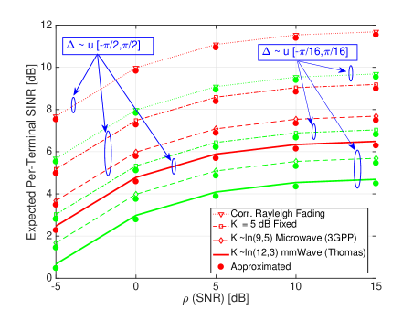
First, the accuracy of the proposed expected per-terminal SINR in
(17) is examined. Fig. 1 illustrates
the expected SINR of a given terminal as a function of (SNR)
for a system with and , and .
In addition to the microwave and
mmWave cases, we consider the correlated Rayleigh fading case
for comparison purposes. We also consider the case where each terminal
is assigned a fixed -factor of dB. Three trends can be observed:
Firstly, transitioning from large to small angular spread
(
to
tends to significantly reduce the expected SINR for all cases. This is
despite the fact that the ULA contains
very large numbers of antenna elements at the BS,
and is due to the reduction in the spatial diversity (rank) of the channel,
allowing the BS array to only see a very narrow spread of
incoming power. Secondly, increasing the mean of has an adverse effect
on the expected SINR. This is because a stronger specular component in
the channel tends to reduce the multipath diversity and in-turn reduces
its overall rank. Equivalently, this can be interpreted as an increase in
the level of inter-terminal interference leading to a lower expected
per-terminal SINR.
Third, our proposed approximations are seen to remain extremely tight
for the entire SNR range for all cases. The analytical expressions are also
seen to
remain tight for the special case presented in (19), where
each terminal undergoes Rayleigh fading with unequal correlation matrices.
Furthermore, the expected SINR in each case is seen to saturate with
growing SNR, due to the inability of the MRC to mitigate inter-terminal
interference.
Figure 1: Expected per-terminal SINR vs. (SNR)
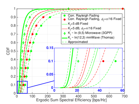
with .Figure 2: Ergodic sum spectral efficiency CDF with , dB, and
(unless specified in
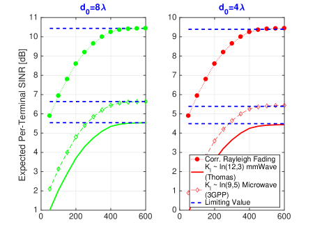
the figure).Figure 3: Expected Per-Terminal SINR vs. with at
(SNR) dB, ,
.
Considering the special cases in (20) and (21),
we now examine the influence of LoS, as well as equal and unequal
correlation matrices on the ergodic sum spectral efficiency, as
shown in Fig. 2. Using the same propagation parameters from
Fig. 1,
(listed in the figure caption) at (SNR) dB,
we compare the cumulative distribution functions (CDFs)
of the derived ergodic sum spectral efficiency approximation in
(18) with its simulated counterparts. We note that the
CDF is obtained by averaging over the
fast-fading in the channel with each value representing the variations
in the link gains and -factors. We notice that
irrespective of the underlaying propagation characteristics
(Rayleigh or Ricean fading), unequal correlation matrices results in a
higher ergodic sum spectral efficiency of the system allowing the ULA to
leverage a larger amount of spatial diversity. Furthermore, we again
observe that a stronger specular component tends to decrease the ergodic
sum spectral efficiency. The derived approximations are robust to the
presence of equal and unequal correlation matrices, as well as changes in
the level of LoS.
We also evaluate the accuracy of the limiting expected SINR expression
derived in (36), with growing numbers of BS antennas and a
fixed number of terminals in the system at . Three trends can be
observed: After recognizing that increasing increases the expected
SINR, for each case the expected SINR slowly
saturates with growing and approaches its limiting value at
approximately 500 antenna elements for each case, respectively. This is a
result of channels from multiple terminals becoming asymptotically
orthogonal. Secondly, decreasing the physical size of the array further
reduces the inter-element spacing translating into a reduction in the
expected SINR for all cases respectively. Finally, we can observe
that each case converges to the derived limiting value.
VII Conclusion
In this paper, we investigated the uplink performance of large MU-MIMO
systems under spatially correlated Ricean fading,
with ULAs at the BS employed in a fixed physical space. Closed-form
approximations to the expected per-terminal SINR and ergodic sum spectral
efficiency are derived with MRC processing at the BS. In the limit of a
large number of BS antennas, asymptotic expressions for the expected
per-terminal SINR
and ergodic sum spectral efficiency were derived. Our numerical results
show that with constraints on the physical size of the ULA, the expected
SINR saturated with increasing SNR and BS antenna numbers. The analysis
accommodates to changes in system dimensions, operating SNR, LoS levels,
spatial correlation levels and variation in fixed physical spacings.
Unequal correlation matrices to each terminal resulted in a performance
increase, whilst LoS had an adverse impact on system performance.
Appendix A Proof of Lemma 1
We begin by recognizing
.
Substituting the definition of and
denoting and
allows us to
state
Performing the expectation over in the last four
terms of (39) and simplifying yields
(40)
After recognizing that , substituting the definition of and extracting the relevant
constants allows us to write
(41)
where is an eigenvalue decomposition of
. As a result,
(42)
where denotes the -th element of .
Performing the expectation with respect to and further
simplifying yields
(43)
This allows us to write
(44)
Recognizing that
allows us to state
(45)
Substituting the definition of back, recognizing that
,
combining (45) with the remaining terms in (40)
and extracting the relevant constants results in the desired expression.
Appendix B Proof of Lemma 2
Applying the definition of and into
and denoting
and
yields
Invoking the independence between and , recognizing
that ,
upon substituting back the definitions of and and extracting the
relevant constants, we can state
(49)
Taking the trace and simplifying yields
the result in (12).
Acknowledgment
The authors would like to thank Prof. Andreas F. Molisch at
the University of Southern California for the insightful
discussions during the course of this work.
References
[1] F. Rusek, D. Persson, B. Lau, E. G. Larsson, T. L. Marzetta, O. Edfors, and F. Tufvesson, “Scaling up MIMO: Opportunities and challenges with very large arrays”, IEEE Signal Process. Mag., vol. 30, no. 1, pp. 40-60, Nov. 2013.
[2] E. G. Larsson, O. Edfors, F. Tufvesson, and T. L. Marzetta, “Massive MIMO for next generation wireless systems”, IEEE Commun. Mag., vol. 52, no. 2, pp. 186-195, Feb. 2014.
[3] C. Masouros, M. Sellathurai, and T. Ratnarajah, “Large-scale MIMO transmitters in fixed physical spaces: The effect of transmit correlation and mutual coupling”, IEEE Trans. Commun., vol. 61, no. 7, pp. 2794-2804, Jul. 2013.
[4] C. Masouros and M. Matthaiou, “Space-constrained massive MIMO: Hitting the wall of favorable propagation”, IEEE Commun. Lett., vol. 19, no. 5, pp. 771-774, May 2015.
[5] H. Q. Ngo, E. G. Larsson, and T. L. Marzetta, “The multicell multiuser
MIMO uplink with very large antenna arrays and a finite-dimensional channel”,
IEEE Trans. Commun., vol. 6, no. 61, pp. 2350-2361, Jun. 2013.
[6] A. Garcia-Rodriguez and C. Masouros, “Exploiting the increasing correlation of space constrained massive MIMO for CSI relaxation”,
IEEE Trans. Commun., vol. 4, no. 64, pp. 1572-1587, Apr. 2016.
[7] J. Zhang, L. Dai, M. Matthaiou, C. Masouros, and S. Jin, “On the spectral efficiency of space-constrained massive MIMO with linear receivers”, in
Proc. of IEEE Int. Conf. on Commun. (ICC), pp. 1-6, May 2016.
[8] S. Biswas, C. Masouros, and T. Ratnarajah, “Performance analysis of large multi-user MIMO systems with space-constrained 2D antenna arrays”,
IEEE Trans. Wireless Commun., vol. 15, no. 5, pp. 3492-3505, May 2016.
[9] X. Ge, R. Zi, H. Wang, J. Zhang, and M. Jo, “Multi-user massive MIMO communication systems based on irregular antenna arrays”, IEEE Trans. Wireless Commun., vol. 15, no. 8, pp. 5287-5301, Aug. 2016.
[10] M. R. Akdeniz, Y. Liu, M. K. Samimi, S. Sun, S. Rangan, T. S. Rappaport, and E. Erkip, “Millimeter wave channel modeling and cellular capacity evaluation”, IEEE J. Sel. Areas Commun., vol. 32, no. 6, pp. 1164-1179, Jun. 2014.
[11] S. Sun, T. S. Rappaport, R. W. Heath Jr., A. R. Nix, and S. Rangan, “MIMO for millimeter-wave wireless communications: Beamforming, spatial multiplexing, or both?”, IEEE Commun. Mag., vol. 52, no. 12, pp. 110-121, Dec. 2014.
[12] H. Tataria, P. J. Smith, L. J. Greenstein, P. A. Dmochowski, and M. Shafi, “Performance and analysis of downlink multiuser MIMO systems with regularized zero-forcing precoding in Ricean fading channels”, in Proc. of IEEE Int. Conf. on Commun. (ICC), pp. 1185-1192, May 2016.
[13] H. Tataria, P. J. Smith, L. J. Greenstein, and P. A. Dmochowski,
“Zero-forcing precoding performance in multiuser MIMO systems with heterogeneous Ricean fading”, IEEE Wireless Commun. Lett., vol. 6, no. 1, pp. 74-77, Feb. 2017.
[14] J. Nam, G. Caire, and J. Ha, “On the role of transmit correlation diversity in multiuser MIMO systems”, IEEE Trans. Info. Theory, vol. 63, no. 1, pp. 336-354, Jan. 2017.
[15] A. F. Molisch Wireless Communications, Wiley Press, 2011.
[16] K. Warnick and M. Jensen, “Optimal noise matching for mutually coupled arrays”, IEEE Trans. Antennas Propag., vol. 55, no. 6, pp. 1726-1731, Jun. 2007.
[17] 3GPP TR 36.873 v12.0.0, Study on 3D channel models for LTE,
3GPP, Jun. 2015.
[18] Q. Zhang, S. Jin, K-K. Wong, H. Zhu, and M. Matthaiou, “Power scaling of uplink massive MIMO systems with arbitrary-rank channel means”, IEEE J. Sel. Topics Signal Process., vol. 8, no. 5, pp. 966-981, Nov. 2014.
[19] D. Basnayaka, P. J. Smith, and P. A. Martin, “Performance analysis of macrodiversity MIMO systems with MMSE and ZF receivers in flat Rayleigh fading”, IEEE Trans. Wireless Commun., vol. 12, no. 5, pp. 2240-2251, May 2013.
[20] T. Thomas, H. C. Nguyen, G. R. MacCartney, and T. S. Rappaport,
“3D mmWave channel model proposal”, in Proc. IEEE Conf. on Veh. Technol. (VTC-Fall), pp. 1-6, Sep. 2014.