$0^{+}$ tetraquark states from improved QCD sum rules: delving into $X(5568)$

Abstract

In order to investigate the possibility of the recently observed $X(5568)$ being a $0^{+}$ tetraquark state, we make an improvement to the study of the related various configuration states in the framework of the QCD sum rules. Particularly, to ensure the quality of the analysis, condensates up to dimension $12$ are included to inspect the convergence of operator product expansion (OPE) and improve the final results of the studied states. We note that some condensate contributions could play an important role on the OPE side. By releasing the rigid OPE convergence criterion, we arrive at the numerical value $5.57^{+0.35}_{-0.23}~{}\mbox{GeV}$ for the scalar-scalar diquark-antidiquark $0^{+}$ state, which agrees with the experimental data for the $X(5568)$ and could support its interpretation in terms of a $0^{+}$ tetraquark state with the scalar-scalar configuration. The corresponding result for the axial-axial current is calculated to be $5.77^{+0.44}_{-0.33}~{}\mbox{GeV}$, which is still consistent with the mass of $X(5568)$ in view of the uncertainty. The feasibility of $X(5568)$ being a tetraquark state with the axial-axial configuration therefore cannot be definitely excluded. For the pseudoscalar-pseudoscalar and the vector-vector cases, their unsatisfactory OPE convergence make it difficult to find reasonable work windows to extract the hadronic information.

I Introduction

Not long ago, the D0 Collaboration reported evidence for a narrow structure, referred to as the $X(5568)$, in the decay modes $X(5568)\rightarrow B_{s}^{0}\pi^{\pm}$ produced in $p\bar{p}$ collisions at center-of-mass energy $\sqrt{s}=1.96~{}\mbox{TeV}$ X5568 . Its mass and natural width were measured to be $m=5567.8\pm 2.9_{-1.9}^{+0.9}~{}\mbox{MeV}$ and $\Gamma=21.9\pm 6.4_{-2.5}^{+5.0}~{}\mbox{MeV}$, respectively. With the $B_{s}^{0}\pi^{+}$ produced in an $S$-wave, its quantum number would be $J^{P}=0^{+}$. Subsequently, the LHCb Collaboration announced that the existence of $X(5568)$ was not confirmed in the analysis of $pp$ collision at energies $7~{}\mbox{TeV}$ and $8~{}\mbox{TeV}$ X5568-1 , and the CMS Collaboration did not find the $X(5568)$ structure X5568-2 either. However, the D0 Collaboration then observed the $X(5568)$ again in the $B_{s}^{0}\pi^{\pm}$ invariant mass distribution via another channel $B_{s}^{0}\rightarrow D_{s}\mu\nu$ at the same mass and at the expected width and rate X5568-3 . One explanation for the $X(5568)$ appearance in D0 and its absence in LHCb and CMS was proposed in Ref. X5568-4 .

The $X(5568)$ has not only attracted experimental attention, but also aroused great enthusiasm from theorists in attempting to understand its underlying structure X5568-Tetra ; X5568-Th (for recent reviews, see e.g. Refs. X5568-rev ; X5568-rev1 and references therein). As an imaginable scenario, a $0^{+}$ tetraquark state with four different valence quark flavors has been proposed as a potential candidate X5568 ; X5568-Tetra . Without doubt, it is important to investigate whether $X(5568)$ can be interpreted as a tetraquark state, which could provide a crucial piece of information to help understand how exotic hadrons are bound, and comprehend QCD more deeply at low energy. However, it is difficult to quantitatively acquire the hadronic information, in view of our limited understanding of QCD’s nonperturbative aspects.

The QCD sum rule approach svzsum is a nonperturbative formulation firmly grounded on the QCD theory, which has already been widely and successfully applied to research many hadrons overview1 ; overview2 ; overview3 ; overview4 . With regard to the recently observed $X(5568)$, there have been several studies using the QCD sum rules to study its mass from the point of view of a $0^{+}$ tetraquark state Azizi ; Wang ; Zhu ; Nielsen ; Qiao ; Narison , chiefly focusing on some particular configurations. Firstly, one can employ various configurations, e.g. scalar-scalar, pseudoscalar-pseudoscalar, axial vector-axial vector (shortened to “axial-axial” below), and vector-vector diquark-antidiquark, to construct a $0^{+}$ tetraquark current and work over these possible configurations. Secondly, for the QCD sum rule method, one of its key points is that both the OPE convergence and the pole dominance should be meticulously inspected to determine the work window, ensuring the credibility of the obtained result. It may be difficult to satisfy both the above criteria, because in some cases it may be hard to find a work window critically satisfying both rules. This could become specially obvious for some multiquark states (e.g. see discussions in Refs. Zs0 ; Zs1 ; Zs2 ; Zs ). The main reason is that some high dimension condensates may play an important role on the OPE side, which means that the standard OPE convergence may happen only at large values of the Borel parameters. Therefore, it may be more reliable to test the OPE convergence by taking into account higher dimension condensates and fixing the work windows precisely. One can then obtain the hadronic properties more safely. Even if higher condensates do not radically influence the character of OPE convergence in some cases, to say the least, one still could expect to improve the final result, since higher dimensional condensates are helpful to stabilize the Borel curve. In order to uncover the inner structure of $X(5568)$, it is significant and worthwhile to make further theoretical efforts. From the above two considerations, we endeavor to perform an improved sum rule study on whether $X(5568)$ could be a $0^{+}$ tetraquark state. In particular, we carry out calculations with four different configuration currents and pay close attention to higher dimension condensate effects.

The rest of this paper is organized as follows. In Section II, QCD sum rules for the tetraquark states are derived, involving both the phenomenological representation and the QCD side, which is followed by numerical analysis and some discussion in Section III. The last section give a brief summary.

II Tetraquark state QCD sum rules

In the QCD sum rules, one basic point is to build a proper interpolating current to represent the studied state. For a tetraquark state, its current could be constructed as the usual diquark-antidiquark configuration. Hence, one can obtain the following form of current:

$$j_{(i)} = \epsilon_{abc}\epsilon_{dec}(q_{a}^{T}\Gamma_{i}s_{b})(\bar{q}_{d}\Gamma^{\prime}_{i}\bar{Q}_{e}^{T})$$

for the tetraquark sate, where the index $i$ takes $I,II,III$, or $IV$, $q$ indicates the light $u$ or $d$ quark, $Q$ denotes the heavy quark, and the subscripts $a$, $b$, $c$, $d$, and $e$ are color indices. To form currents with a total quantum number $J^{P}=0^{+}$, $\Gamma$ matrices are taken as $\Gamma_{I}=C\gamma_{5}$, $\Gamma^{\prime}_{I}=\gamma_{5}C$ for the scalar-scalar case, $\Gamma_{II}=C$, $\Gamma^{\prime}_{II}=C$ for the pseudoscalar-pseudoscalar case, $\Gamma_{III}=C\gamma_{\mu}$, $\Gamma^{\prime}_{III}=\gamma^{\mu}C$ for the axial-axial case, and $\Gamma_{IV}=C\gamma_{5}\gamma_{\mu}$, $\Gamma^{\prime}_{IV}=\gamma^{\mu}\gamma_{5}C$ for the vector-vector case.

Further, the two-point correlator,

$$\Pi_{i}(q^{2})=i\int d^{4}x\mbox{e}^{iq.x}\langle 0|T[j_{(i)}(x)j_{(i)}^{{\dagger}}(0)]|0\rangle,$$ (1)

can be used to derive the tetraquark state QCD sum rules.

The correlator $\Pi_{i}(q^{2})$ can be phenomenologically expressed as

$$\Pi_{i}(q^{2})=\frac{\lambda_{H}^{2}}{M_{H}^{2}-q^{2}}+\frac{1}{\pi}\int_{s_{0}}^{\infty}\frac{\mbox{Im}\big{[}\Pi_{i}^{\mbox{phen}}(s)\big{]}}{s-q^{2}}ds+...,$$ (2)

where $M_{H}$ is the mass of the hadronic state, $s_{0}$ denotes the continuum threshold, and $\lambda_{H}$ indicates the coupling of the current to the hadron $\langle 0|j|H\rangle=\lambda_{H}$.

On the OPE side, the correlator $\Pi_{i}(q^{2})$ can be theoretically written as

$$\Pi_{i}(q^{2})=\int_{(m_{Q}+m_{s})^{2}}^{\infty}\frac{\rho_{i}(s)}{s-q^{2}}ds+\Pi_{i}^{\mbox{cond}}(q^{2}),$$ (3)

where the spectral density $\rho_{i}(s)$ is $\frac{1}{\pi}\mbox{Im}\big{[}\Pi_{i}(s)\big{]}$, $m_{Q}$ is the heavy quark mass, and $m_{s}$ is the strange quark mass. In the concrete derivation, one can work at leading order in $\alpha_{s}$ and take into account condensates up to dimension $12$, with similar techniques as in Refs. overview4 ; Tech ; Zhang . To keep the heavy-quark mass $m_{Q}$ finite, one can use the heavy-quark propagator in the momentum space reinders ,

$$S_{Q}(p) = \frac{i}{\hbox to0.0pt{/\hss}p-m_{Q}}-\frac{i}{4}gt^{A}G^{A}_{\kappa\lambda}(0)\frac{1}{(p^{2}-m_{Q}^{2})^{2}}\Big{[}\sigma^{\kappa\lambda}(\hbox to0.0pt{/\hss}p+m_{Q})+(\hbox to0.0pt{/\hss}p+m_{Q})\sigma^{\kappa\lambda}\Big{]}$$

$${}-\frac{i}{4}g^{2}t^{A}t^{B}G^{A}_{\alpha\beta}(0)G^{B}_{\mu\nu}(0)\frac{\hbox to0.0pt{/\hss}p+m_{Q}}{(p^{2}-m_{Q}^{2})^{5}}\Big{[}\gamma^{\alpha}(\hbox to0.0pt{/\hss}p+m_{Q})\gamma^{\beta}(\hbox to0.0pt{/\hss}p+m_{Q})\gamma^{\mu}(\hbox to0.0pt{/\hss}p+m_{Q})\gamma^{\nu}$$

$${}+\gamma^{\alpha}(\hbox to0.0pt{/\hss}p+m_{Q})\gamma^{\mu}(\hbox to0.0pt{/\hss}p+m_{Q})\gamma^{\beta}(\hbox to0.0pt{/\hss}p+m_{Q})\gamma^{\nu}+\gamma^{\alpha}(\hbox to0.0pt{/\hss}p+m_{Q})\gamma^{\mu}(\hbox to0.0pt{/\hss}p+m_{Q})\gamma^{\nu}(\hbox to0.0pt{/\hss}p+m_{Q})\gamma^{\beta}\Big{]}(\hbox to0.0pt{/\hss}p+m_{Q})$$

$${}+\frac{i}{48}g^{3}f^{ABC}G^{A}_{\gamma\delta}G^{B}_{\delta\varepsilon}G^{C}_{\varepsilon\gamma}\frac{1}{(p^{2}-m_{Q}^{2})^{6}}(\hbox to0.0pt{/\hss}p+m_{Q})\Big{[}\hbox to0.0pt{/\hss}p(p^{2}-3m_{Q}^{2})+2m_{Q}(2p^{2}-m_{Q}^{2})\Big{]}(\hbox to0.0pt{/\hss}p+m_{Q}).$$

The light-quark part of the correlator can be calculated in the coordinate space, with the light-quark propagator,

$$S_{ab}(x) = \frac{i\delta_{ab}}{2\pi^{2}x^{4}}\hbox to0.0pt{/\hss}x-\frac{m_{q}\delta_{ab}}{4\pi^{2}x^{2}}-\frac{i}{32\pi^{2}x^{2}}t^{A}_{ab}gG^{A}_{\mu\nu}(\hbox to0.0pt{/\hss}x\sigma^{\mu\nu}+\sigma^{\mu\nu}\hbox to0.0pt{/\hss}x)-\frac{\delta_{ab}}{12}\langle\bar{q}q\rangle+\frac{i\delta_{ab}}{48}m_{q}\langle\bar{q}q\rangle\hbox to0.0pt{/\hss}x$$ (5)

$${}-\frac{x^{2}\delta_{ab}}{3\cdot 2^{6}}\langle g\bar{q}\sigma\cdot Gq\rangle+\frac{ix^{2}\delta_{ab}}{2^{7}\cdot 3^{2}}m_{q}\langle g\bar{q}\sigma\cdot Gq\rangle\hbox to0.0pt{/\hss}x-\frac{x^{4}\delta_{ab}}{2^{10}\cdot 3^{3}}\langle\bar{q}q\rangle\langle g^{2}G^{2}\rangle,$$

which is then Fourier-transformed to the momentum space in $D$ dimensions. The strange quark is treated as a light one and the diagrams are considered up to order $m_{s}$. The resulting light-quark part is combined with the heavy-quark part before it is dimensionally regularized at $D=4$. After equating Eqs. (2) and (3), utilizing quark-hadron duality, and doing a Borel transform $\hat{B}$, the sum rule can be

$$\lambda_{H}^{2}e^{-M_{H}^{2}/M^{2}} = \int_{(m_{Q}+m_{s})^{2}}^{s_{0}}\rho_{i}(s)e^{-s/M^{2}}ds+\hat{B}\Pi_{i}^{\mbox{cond}},$$ (6)

with $M^{2}$ the Borel parameter. For compactness, the concrete forms of $\rho_{i}(s)$ and $\hat{B}\Pi_{i}^{\mbox{cond}}$ are shown in the Appendix.

Taking the derivative of the sum rule (6) in terms of $-\frac{1}{M^{2}}$ and then dividing by itself, one can get the mass of the hadronic state

$$M_{H} = \sqrt{\bigg{\{}\int_{(m_{Q}+m_{s})^{2}}^{s_{0}}\rho_{i}(s)se^{-s/M^{2}}ds+\frac{d\big{(}\hat{B}\Pi_{i}^{\mbox{cond}}\big{)}}{d(-\frac{1}{M^{2}})}\bigg{\}}/\bigg{\{}\int_{(m_{Q}+m_{s})^{2}}^{s_{0}}\rho_{i}(s)e^{-s/M^{2}}ds+\hat{B}\Pi_{i}^{\mbox{cond}}\bigg{\}}},$$ (7)

with $i=I$, $II$, $III$, or $IV$.

III Numerical analysis and discussion

In this section, we perform numerical analysis of the sum rule (7) to extract the mass value of the studied state. The input parameters are taken as $m_{b}=4.18^{+0.04}_{-0.03}~{}\mbox{GeV}$, $m_{s}=96^{+8}_{-4}~{}\mbox{MeV}$, $\langle\bar{q}q\rangle=-(0.24\pm 0.01)^{3}~{}\mbox{GeV}^{3}$, $\langle\bar{s}s\rangle=m_{0}^{2}~{}\langle\bar{q}q\rangle$, $\langle g\bar{q}\sigma\cdot Gq\rangle=m_{0}^{2}~{}\langle\bar{q}q\rangle$, $m_{0}^{2}=0.8\pm 0.1~{}\mbox{GeV}^{2}$, $\langle g^{2}G^{2}\rangle=0.88\pm 0.25~{}\mbox{GeV}^{4}$, and $\langle g^{3}G^{3}\rangle=0.58\pm 0.18~{}\mbox{GeV}^{6}$ PDG ; svzsum ; overview2 . In the standard procedure, one should consider both the OPE convergence and the pole contribution dominance to choose proper work windows for the threshold $\sqrt{s_{0}}$ and the Borel parameter $M^{2}$. At the same time, the threshold $\sqrt{s_{0}}$ cannot be taken optionally. This is because $\sqrt{s_{0}}$ characterizes the beginning of continuum states. In practice, it may be difficult to find a conventional work window that critically satisfies all the rules in some studies (for instance, see Refs. Zs0 ; Zs1 ; Zs2 ; Zs ).

One can illustrate the numerical analysis process by giving the scalar-scalar case as an example. Its various contributions are compared as a function of $M^{2}$ and shown in Fig. 1 to test the convergence of OPE. There are three main condensate contributions, i.e. the two-quark condensate, the four-quark condensate, and the mixed condensate. These condensates could play an important role on the OPE side, which makes the standard OPE convergence happen only at very large values of $M^{2}$. The consequence is that it is difficult to find a conventional Borel window strictly satisfying both that the pole dominates over the continuum and the OPE converges well. It is not too bad for the present case: there are three main condensates and they could cancel each other out to some extent, as they have different signs. What is also very important is that most of other condensates calculated are very small, almost negligible, which means that they cannot radically influence the character of OPE convergence. All these factors mean that one could find the perturbative dominance in the total and the OPE convergence still be under control. Without any adverse consequences, one could try releasing the rigid OPE convergence criterion for the present case and choose proper work windows at relatively low values of $M^{2}$.

On the phenomenological side, the comparison between pole and continuum contributions of sum rule (6) as a function of the Borel parameter $M^{2}$ for the threshold value $\sqrt{s_{0}}=6.1~{}\mbox{GeV}$ is shown in Fig. 2, which shows that the relative pole contribution is approximate to $50\%$ at $M^{2}=3.8~{}\mbox{GeV}^{2}$ and decreases with $M^{2}$. Similarly, the upper bound values of the Borel parameters are $M^{2}=3.7~{}\mbox{GeV}^{2}$ for $\sqrt{s_{0}}=6.0~{}\mbox{GeV}$ and $M^{2}=3.9~{}\mbox{GeV}^{2}$ for $\sqrt{s_{0}}=6.2~{}\mbox{GeV}$. Therefore, the Borel windows for the scalar-scalar diquark-antidiquark state are taken as $2.7\sim 3.7~{}\mbox{GeV}^{2}$ for $\sqrt{s_{0}}=6.0~{}\mbox{GeV}$, $2.7\sim 3.8~{}\mbox{GeV}^{2}$ for $\sqrt{s_{0}}=6.1~{}\mbox{GeV}$, and $2.7\sim 3.9~{}\mbox{GeV}^{2}$ for $\sqrt{s_{0}}=6.2~{}\mbox{GeV}$. The mass of the $0^{+}$ tetraquark state with the scalar-scalar configuration as a function of $M^{2}$ from sum rule (7) is shown in Fig. 3 and it is numerically counted to be $5.57\pm 0.19~{}\mbox{GeV}$ in the chosen work windows. Considering the uncertainty from the variation of quark masses and condensates, we get $5.57\pm 0.19^{+0.16}_{-0.04}~{}\mbox{GeV}$ (the first error reflects the uncertainty due to variation of $\sqrt{s_{0}}$ and $M^{2}$, and the second error results from the variation of QCD parameters) or concisely $5.57^{+0.35}_{-0.23}~{}\mbox{GeV}$ for the scalar-scalar tetraquark state.

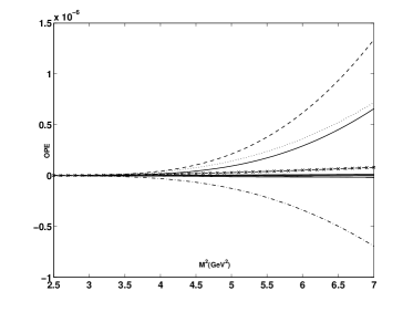
Figure 1: The various OPE contribution as a function of $M^{2}$ in sum rule (6) for $\sqrt{s_{0}}=6.1~{}\mbox{GeV}$ for the scalar-scalar case. Four main contributions, i.e. the perturbative, the two-quark condensate, the four-quark condensate, and the mixed condensate are denoted by the single solid line, the dashed line, the dotted line, and the dot-dashed line, respectively. These main condensates could cancel each other out to some extent, and other condensates are very small. All these factors mean that one can find perturbative dominance in the total and it is still under control for OPE convergence.

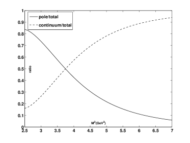
Figure 2: The phenomenological contribution in sum rule (6) for $\sqrt{s_{0}}=6.1~{}\mbox{GeV}$ for the scalar-scalar case. The solid line is the relative pole contribution (the pole contribution divided by the total, pole plus continuum contribution) as a function of $M^{2}$ and the dashed line is the relative continuum contribution.

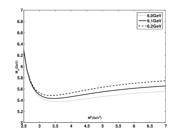
Figure 3: The mass of the $0^{+}$ tetraquark state with the scalar-scalar configuration as a function of $M^{2}$ from sum rule (7). The continuum thresholds are taken as $\sqrt{s_{0}}=6.0\sim 6.2~{}\mbox{GeV}$. The ranges of $M^{2}$ is $2.7\sim 3.7~{}\mbox{GeV}^{2}$ for $\sqrt{s_{0}}=6.0~{}\mbox{GeV}$, $2.7\sim 3.8~{}\mbox{GeV}^{2}$ for $\sqrt{s_{0}}=6.1~{}\mbox{GeV}$, and $2.7\sim 3.9~{}\mbox{GeV}^{2}$ for $\sqrt{s_{0}}=6.2~{}\mbox{GeV}$.

For the axial-axial configuration, the OPE contribution in sum rule (6) for $\sqrt{s_{0}}=6.1~{}\mbox{GeV}$ is shown in Fig. 4 by comparing various contributions. Similarly, the two-quark condensate, the four-quark condensate, and the mixed condensate contributions could cancel each other out to some extent and most of the other condensates calculated are very small. Furthermore, the phenomenological contribution in sum rule (6) for $\sqrt{s_{0}}=6.1~{}\mbox{GeV}$ is displayed in Fig. 5. The work windows for the axial-axial case are taken as $2.9\sim 3.4~{}\mbox{GeV}^{2}$ for $\sqrt{s_{0}}=6.0~{}\mbox{GeV}$, $2.9\sim 3.5~{}\mbox{GeV}^{2}$ for $\sqrt{s_{0}}=6.1~{}\mbox{GeV}$, and $2.9\sim 3.6~{}\mbox{GeV}^{2}$ for $\sqrt{s_{0}}=6.2~{}\mbox{GeV}$. Its Borel curves are shown in Fig. 6 and it is numerically evaluated as $5.77\pm 0.28~{}\mbox{GeV}$ in the work windows. Considering the uncertainty from the variation of quark masses and condensates, we get $5.77\pm 0.28^{+0.16}_{-0.05}~{}\mbox{GeV}$ (the first error characterizes the uncertainty due to variation of $\sqrt{s_{0}}$ and $M^{2}$, and the second error is from the variation of QCD parameters) for the axial-axial tetraquark state, or more concisely, $5.77^{+0.44}_{-0.33}~{}\mbox{GeV}$.

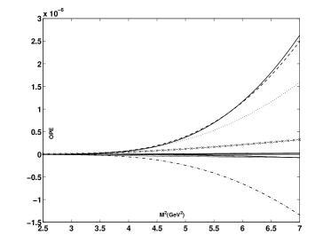
Figure 4: The various OPE contributions as a function of $M^{2}$ in sum rule (6) for $\sqrt{s_{0}}=6.1~{}\mbox{GeV}$ for the axial-axial case. Four main contributions, i.e. the perturbative, the two-quark condensate, the four-quark condensate, and the mixed condensate are denoted by the single solid line, the dashed line, the dotted line, and the dot-dashed line, respectively. These main condensates could cancel each other out to some extent, and other condensates are very small. All these factors mean that one can find perturbative dominance in the total and OPE convergence is still under control.

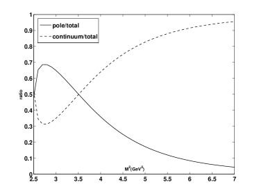
Figure 5: The phenomenological contribution in sum rule (6) for $\sqrt{s_{0}}=6.1~{}\mbox{GeV}$ for the axial-axial case. The solid line is the relative pole contribution (the pole contribution divided by the total, pole plus continuum contribution) as a function of $M^{2}$ and the dashed line is the relative continuum contribution.

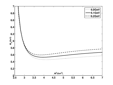
Figure 6: The mass of the $0^{+}$ tetraquark state with the axial-axial configuration as a function of $M^{2}$ from sum rule (7). The continuum thresholds are taken as $\sqrt{s_{0}}=6.0\sim 6.2~{}\mbox{GeV}$. The ranges of $M^{2}$ are $2.9\sim 3.4~{}\mbox{GeV}^{2}$ for $\sqrt{s_{0}}=6.0~{}\mbox{GeV}$, $2.9\sim 3.5~{}\mbox{GeV}^{2}$ for $\sqrt{s_{0}}=6.1~{}\mbox{GeV}$, and $2.9\sim 3.6~{}\mbox{GeV}^{2}$ for $\sqrt{s_{0}}=6.2~{}\mbox{GeV}$.

For the pseudoscalar-pseudoscalar case, the OPE contribution in sum rule (6) for $\sqrt{s_{0}}=6.1~{}\mbox{GeV}$ is shown in Fig. 7. There are also three main condensates, i.e. the two-quark condensate, the four-quark condensate, and the mixed condensate on the OPE side. They can certainly counteract each other to some extent. However, quite different from the two cases discussed above, there are two main condensates (the two-quark condensate and the four-quark condensate) which have a different sign from the perturbative term, which means the signs of the perturbative part and the total OPE contribution are different. The unsatisfactory OPE convergence means it is difficult to find some reasonable work windows for this case. It is inadvisable to keep on evaluating further numerical results. Similarly, the OPE contribution in sum rule (6) for $\sqrt{s_{0}}=6.1~{}\mbox{GeV}$ for the vector-vector case is shown in Fig. 8. It has the same problem as the pseudoscalar-pseudoscalar case, and the most direct consequence is that the Borel curves are rather unstable. Thus, it is also hard to find appropriate work windows to extract credible hadronic information for the vector-vector case.

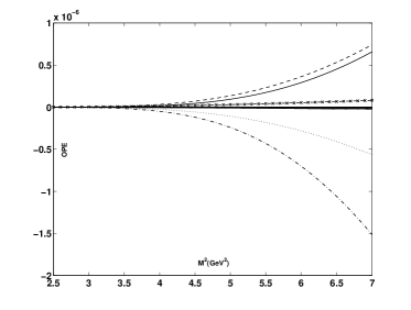
Figure 7: The various OPE contributions as a function of $M^{2}$ in sum rule (6) for $\sqrt{s_{0}}=6.1~{}\mbox{GeV}$ for the pseudoscalar-pseudoscalar case. Four main contributions, i.e. the perturbative, the two-quark condensate, the four-quark condensate, and the mixed condensate are denoted by the single solid line, the dot-dashed line, the dotted line, and the dashed line, respectively. There two main condensates have a different sign from the perturbative term, which means the perturbative part and the total OPE contribution have different signs, and the OPE convergence is not satisfactory for the pseudoscalar-pseudoscalar case.

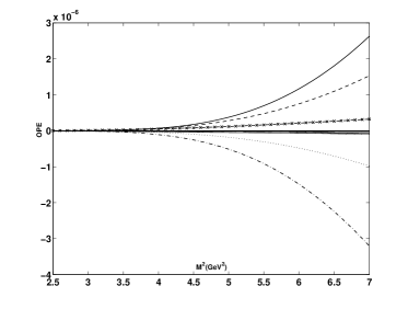
Figure 8: The various OPE contribution as a function of $M^{2}$ in sum rule (6) for $\sqrt{s_{0}}=6.1~{}\mbox{GeV}$ for the vector-vector case. Four main contributions, i.e. the perturbative, the two-quark condensate, the four-quark condensate, and the mixed condensate are denoted by the single solid line, the dot-dashed line, the dotted line, and the dashed line, respectively. There two main condensates have a different sign from the perturbative term, which means the perturbative part and the total OPE contribution have different signs, and the OPE convergence is not satisfactory for the vector-vector case.

IV Summary

Stimulated by the possibility of the recently observed structure $X(5568)$ being an ideal candidate for exotic hadrons, we present an improved QCD sum rule study to investigate whether $X(5568)$ could be a $0^{+}$ tetraquark state. In deriving the sum rules, we have used four different interpolating currents, i.e. the scalar-scalar, the pseudoscalar-pseudoscalar, the axial-axial, and the vector-vector diquark-antidiquark configurations. Furthermore, in order to ensure the quality of QCD sum rule analysis, contributions of condensates up to dimension $12$ are computed to test the OPE convergence. We find that some condensates, such as the two-quark condensate, the four-quark condensate, and the mixed condensate, could play an important role on the OPE side. The effect is not too bad for the scalar-scalar and the axial-axial cases, as their main condensates could cancel each other out to some extent. Most of the other condensates calculated are very small, almost negligible, which means that they cannot radically influence the character of OPE convergence. All these factors mean that the OPE convergence for the scalar-scalar and the axial-axial cases is still controllable.

Releasing the rigid OPE convergence criterion gives the following outcomes. 1) The final result for the scalar-scalar case is $5.57^{+0.35}_{-0.23}~{}\mbox{GeV}$, which coincides with the experimental data of $X(5568)$. This result therefore supports the tetraquark state explanation of $X(5568)$ with the scalar-scalar configuration. 2) For the axial-axial case, its eventual numerical value is $5.77^{+0.44}_{-0.33}~{}\mbox{GeV}$, which is still consistent with the mass of $X(5568)$ in view of the uncertainty although the central value is slightly higher. Thus, one cannot arbitrarily exclude the possibility of $X(5568)$ being an axial-axial configuration tetraquark state. 3) For the pseudoscalar-pseudoscalar and the vector-vector cases, their OPE convergence is so unsatisfactory that one cannot find appropriate work windows to get reliable hadronic information. In future, it is expected that more precise information on the nature of the $X(5568)$ will be revealed by the further contributions of both experimental observations and theoretical studies.

Appendix A

The spectral density $\rho_{i}(s)$ is

$$\rho_{i}(s)=\rho_{i}^{\mbox{pert}}(s)+\rho_{i}^{\langle\bar{q}q\rangle}(s)+\rho_{i}^{\langle g^{2}G^{2}\rangle}(s)+\rho_{i}^{\langle g\bar{q}\sigma\cdot Gq\rangle}(s)+\rho_{i}^{\langle\bar{q}q\rangle^{2}}(s)+\rho_{i}^{\langle g^{3}G^{3}\rangle}(s)+\rho_{i}^{\langle\bar{q}q\rangle\langle g^{2}G^{2}\rangle}(s),$$

with $i=I$, $II$, $III$, and $IV$. Concretely,

$$\rho_{I}^{\mbox{pert}}(s) = \frac{1}{3\cdot 2^{10}\pi^{6}}\int_{\Lambda}^{1}d\alpha\bigg{(}\frac{1-\alpha}{\alpha}\bigg{)}^{3}(\alpha s-m_{Q}^{2})^{4},$$

$$\rho_{II}^{\mbox{pert}}(s) = \frac{1}{3\cdot 2^{10}\pi^{6}}\int_{\Lambda}^{1}d\alpha\bigg{(}\frac{1-\alpha}{\alpha}\bigg{)}^{3}(\alpha s-m_{Q}^{2})^{4},$$

$$\rho_{III}^{\mbox{pert}}(s) = \frac{1}{3\cdot 2^{8}\pi^{6}}\int_{\Lambda}^{1}d\alpha\bigg{(}\frac{1-\alpha}{\alpha}\bigg{)}^{3}(\alpha s-m_{Q}^{2})^{4},$$

$$\rho_{IV}^{\mbox{pert}}(s) = \frac{1}{3\cdot 2^{8}\pi^{6}}\int_{\Lambda}^{1}d\alpha\bigg{(}\frac{1-\alpha}{\alpha}\bigg{)}^{3}(\alpha s-m_{Q}^{2})^{4},$$

$$\rho_{I}^{\langle\bar{q}q\rangle}(s) = \frac{1}{2^{6}\pi^{4}}\int_{\Lambda}^{1}d\alpha\bigg{(}m_{s}\langle\bar{s}s\rangle-2m_{s}\langle\bar{q}q\rangle-m_{Q}\langle\bar{q}q\rangle\frac{1-\alpha}{\alpha}\bigg{)}\frac{1-\alpha}{\alpha}(\alpha s-m_{Q}^{2})^{2},$$

$$\rho_{II}^{\langle\bar{q}q\rangle}(s) = \frac{1}{2^{6}\pi^{4}}\int_{\Lambda}^{1}d\alpha\bigg{(}m_{s}\langle\bar{s}s\rangle+2m_{s}\langle\bar{q}q\rangle+m_{Q}\langle\bar{q}q\rangle\frac{1-\alpha}{\alpha}\bigg{)}\frac{1-\alpha}{\alpha}(\alpha s-m_{Q}^{2})^{2},$$

$$\rho_{III}^{\langle\bar{q}q\rangle}(s) = \frac{1}{2^{4}\pi^{4}}\int_{\Lambda}^{1}d\alpha\bigg{(}m_{s}\langle\bar{s}s\rangle-m_{s}\langle\bar{q}q\rangle-\frac{1}{2}m_{Q}\langle\bar{q}q\rangle\frac{1-\alpha}{\alpha}\bigg{)}\frac{1-\alpha}{\alpha}(\alpha s-m_{Q}^{2})^{2},$$

$$\rho_{IV}^{\langle\bar{q}q\rangle}(s) = \frac{1}{2^{4}\pi^{4}}\int_{\Lambda}^{1}d\alpha\bigg{(}m_{s}\langle\bar{s}s\rangle+m_{s}\langle\bar{q}q\rangle+\frac{1}{2}m_{Q}\langle\bar{q}q\rangle\frac{1-\alpha}{\alpha}\bigg{)}\frac{1-\alpha}{\alpha}(\alpha s-m_{Q}^{2})^{2},$$

$$\rho_{I}^{\langle g^{2}G^{2}\rangle}(s) = -\frac{m_{Q}^{2}\langle g^{2}G^{2}\rangle}{3^{2}\cdot 2^{10}\pi^{6}}\int_{\Lambda}^{1}d\alpha\bigg{(}\frac{1-\alpha}{\alpha}\bigg{)}^{3}(\alpha s-m_{Q}^{2}),$$

$$\rho_{II}^{\langle g^{2}G^{2}\rangle}(s) = -\frac{m_{Q}^{2}\langle g^{2}G^{2}\rangle}{3^{2}\cdot 2^{10}\pi^{6}}\int_{\Lambda}^{1}d\alpha\bigg{(}\frac{1-\alpha}{\alpha}\bigg{)}^{3}(\alpha s-m_{Q}^{2}),$$

$$\rho_{III}^{\langle g^{2}G^{2}\rangle}(s) = -\frac{m_{Q}^{2}\langle g^{2}G^{2}\rangle}{3^{2}\cdot 2^{8}\pi^{6}}\int_{\Lambda}^{1}d\alpha\bigg{(}\frac{1-\alpha}{\alpha}\bigg{)}^{3}(\alpha s-m_{Q}^{2}),$$

$$\rho_{IV}^{\langle g^{2}G^{2}\rangle}(s) = -\frac{m_{Q}^{2}\langle g^{2}G^{2}\rangle}{3^{2}\cdot 2^{8}\pi^{6}}\int_{\Lambda}^{1}d\alpha\bigg{(}\frac{1-\alpha}{\alpha}\bigg{)}^{3}(\alpha s-m_{Q}^{2}),$$

$$\rho_{I}^{\langle g\bar{q}\sigma\cdot Gq\rangle}(s) = -\frac{1}{3\cdot 2^{6}\pi^{4}}\int_{\Lambda}^{1}d\alpha\bigg{(}m_{s}\langle g\bar{s}\sigma\cdot Gs\rangle-3m_{s}\langle g\bar{q}\sigma\cdot Gq\rangle-3m_{Q}\langle g\bar{q}\sigma\cdot Gq\rangle\frac{1-\alpha}{\alpha}\bigg{)}(\alpha s-m_{Q}^{2}),$$

$$\rho_{II}^{\langle g\bar{q}\sigma\cdot Gq\rangle}(s) = -\frac{1}{3\cdot 2^{6}\pi^{4}}\int_{\Lambda}^{1}d\alpha\bigg{(}m_{s}\langle g\bar{s}\sigma\cdot Gs\rangle+3m_{s}\langle g\bar{q}\sigma\cdot Gq\rangle+3m_{Q}\langle g\bar{q}\sigma\cdot Gq\rangle\frac{1-\alpha}{\alpha}\bigg{)}(\alpha s-m_{Q}^{2}),$$

$$\rho_{III}^{\langle g\bar{q}\sigma\cdot Gq\rangle}(s) = -\frac{1}{3\cdot 2^{4}\pi^{4}}\int_{\Lambda}^{1}d\alpha\bigg{(}m_{s}\langle g\bar{s}\sigma\cdot Gs\rangle-\frac{3}{2}m_{s}\langle g\bar{q}\sigma\cdot Gq\rangle-\frac{3}{2}m_{Q}\langle g\bar{q}\sigma\cdot Gq\rangle\frac{1-\alpha}{\alpha}\bigg{)}(\alpha s-m_{Q}^{2}),$$

$$\rho_{IV}^{\langle g\bar{q}\sigma\cdot Gq\rangle}(s) = -\frac{1}{3\cdot 2^{4}\pi^{4}}\int_{\Lambda}^{1}d\alpha\bigg{(}m_{s}\langle g\bar{s}\sigma\cdot Gs\rangle+\frac{3}{2}m_{s}\langle g\bar{q}\sigma\cdot Gq\rangle+\frac{3}{2}m_{Q}\langle g\bar{q}\sigma\cdot Gq\rangle\frac{1-\alpha}{\alpha}\bigg{)}(\alpha s-m_{Q}^{2}),$$

$$\rho_{I}^{\langle\bar{q}q\rangle^{2}}(s) = \frac{1}{3\cdot 2^{3}\pi^{2}}\int_{\Lambda}^{1}d\alpha\langle\bar{q}q\rangle\Big{[}2\langle\bar{s}s\rangle(\alpha s-m_{Q}^{2})+2m_{Q}m_{s}\langle\bar{q}q\rangle-m_{Q}m_{s}\langle\bar{s}s\rangle\Big{]},$$

$$\rho_{II}^{\langle\bar{q}q\rangle^{2}}(s) = \frac{1}{3\cdot 2^{3}\pi^{2}}\int_{\Lambda}^{1}d\alpha\langle\bar{q}q\rangle\Big{[}-2\langle\bar{s}s\rangle(\alpha s-m_{Q}^{2})+2m_{Q}m_{s}\langle\bar{q}q\rangle+m_{Q}m_{s}\langle\bar{s}s\rangle\Big{]},$$

$$\rho_{III}^{\langle\bar{q}q\rangle^{2}}(s) = \frac{1}{3\cdot 2^{2}\pi^{2}}\int_{\Lambda}^{1}d\alpha\langle\bar{q}q\rangle\Big{[}2\langle\bar{s}s\rangle(\alpha s-m_{Q}^{2})+4m_{Q}m_{s}\langle\bar{q}q\rangle-m_{Q}m_{s}\langle\bar{s}s\rangle\Big{]},$$

$$\rho_{IV}^{\langle\bar{q}q\rangle^{2}}(s) = \frac{1}{3\cdot 2^{2}\pi^{2}}\int_{\Lambda}^{1}d\alpha\langle\bar{q}q\rangle\Big{[}-2\langle\bar{s}s\rangle(\alpha s-m_{Q}^{2})+4m_{Q}m_{s}\langle\bar{q}q\rangle+m_{Q}m_{s}\langle\bar{s}s\rangle\Big{]},$$

$$\rho_{I}^{\langle g^{3}G^{3}\rangle}(s) = -\frac{\langle g^{3}G^{3}\rangle}{3^{2}\cdot 2^{12}\pi^{6}}\int_{\Lambda}^{1}d\alpha\bigg{(}\frac{1-\alpha}{\alpha}\bigg{)}^{3}(\alpha s-3m_{Q}^{2}),$$

$$\rho_{II}^{\langle g^{3}G^{3}\rangle}(s) = -\frac{\langle g^{3}G^{3}\rangle}{3^{2}\cdot 2^{12}\pi^{6}}\int_{\Lambda}^{1}d\alpha\bigg{(}\frac{1-\alpha}{\alpha}\bigg{)}^{3}(\alpha s-3m_{Q}^{2}),$$

$$\rho_{III}^{\langle g^{3}G^{3}\rangle}(s) = -\frac{\langle g^{3}G^{3}\rangle}{3^{2}\cdot 2^{10}\pi^{6}}\int_{\Lambda}^{1}d\alpha\bigg{(}\frac{1-\alpha}{\alpha}\bigg{)}^{3}(\alpha s-3m_{Q}^{2}),$$

$$\rho_{IV}^{\langle g^{3}G^{3}\rangle}(s) = -\frac{\langle g^{3}G^{3}\rangle}{3^{2}\cdot 2^{10}\pi^{6}}\int_{\Lambda}^{1}d\alpha\bigg{(}\frac{1-\alpha}{\alpha}\bigg{)}^{3}(\alpha s-3m_{Q}^{2}),$$

$$\rho_{I}^{\langle\bar{q}q\rangle\langle g^{2}G^{2}\rangle}(s) = -\frac{m_{Q}\langle\bar{q}q\rangle\langle g^{2}G^{2}\rangle}{3^{2}\cdot 2^{8}\pi^{4}}\int_{\Lambda}^{1}d\alpha\bigg{[}1+3\bigg{(}\frac{1-\alpha}{\alpha}\bigg{)}^{2}\bigg{]},$$

$$\rho_{II}^{\langle\bar{q}q\rangle\langle g^{2}G^{2}\rangle}(s) = \frac{m_{Q}\langle\bar{q}q\rangle\langle g^{2}G^{2}\rangle}{3^{2}\cdot 2^{8}\pi^{4}}\int_{\Lambda}^{1}d\alpha\bigg{[}1+3\bigg{(}\frac{1-\alpha}{\alpha}\bigg{)}^{2}\bigg{]},$$

$$\rho_{III}^{\langle\bar{q}q\rangle\langle g^{2}G^{2}\rangle}(s) = -\frac{m_{Q}\langle\bar{q}q\rangle\langle g^{2}G^{2}\rangle}{3^{2}\cdot 2^{7}\pi^{4}}\int_{\Lambda}^{1}d\alpha\bigg{[}1+3\bigg{(}\frac{1-\alpha}{\alpha}\bigg{)}^{2}\bigg{]},$$

and

$$\rho_{IV}^{\langle\bar{q}q\rangle\langle g^{2}G^{2}\rangle}(s) = \frac{m_{Q}\langle\bar{q}q\rangle\langle g^{2}G^{2}\rangle}{3^{2}\cdot 2^{7}\pi^{4}}\int_{\Lambda}^{1}d\alpha\bigg{[}1+3\bigg{(}\frac{1-\alpha}{\alpha}\bigg{)}^{2}\bigg{]},$$

with $\Lambda=m_{Q}^{2}/s$.

The $\hat{B}\Pi_{i}^{\mbox{cond}}$ term reads

$$\hat{B}\Pi_{i}^{\mbox{cond}} = \hat{B}\Pi_{i}^{\langle\bar{q}q\rangle^{3}}+\hat{B}\Pi_{i}^{\langle\bar{q}q\rangle\langle g\bar{q}\sigma\cdot Gq\rangle}+\hat{B}\Pi_{i}^{\langle g\bar{q}\sigma\cdot Gq\rangle^{2}}+\hat{B}\Pi_{i}^{\langle\bar{q}q\rangle\langle g^{2}G^{2}\rangle}+\hat{B}\Pi_{i}^{\langle\bar{q}q\rangle\langle g^{3}G^{3}\rangle}+\hat{B}\Pi_{i}^{\langle g^{2}G^{2}\rangle\langle g\bar{q}\sigma\cdot Gq\rangle}$$

$$+ \hat{B}\Pi_{i}^{\langle\bar{q}q\rangle^{2}\langle g\bar{q}\sigma\cdot Gq\rangle}+\hat{B}\Pi_{i}^{\langle\bar{q}q\rangle\langle g^{2}G^{2}\rangle^{2}}+\hat{B}\Pi_{i}^{\langle\bar{q}q\rangle^{2}\langle g^{2}G^{2}\rangle}+\hat{B}\Pi_{i}^{\langle\bar{q}q\rangle^{2}\langle g^{3}G^{3}\rangle}+\hat{B}\Pi_{i}^{\langle\bar{q}q\rangle\langle g^{2}G^{2}\rangle\langle g\bar{q}\sigma\cdot Gq\rangle}+\hat{B}\Pi_{i}^{\langle g^{3}G^{3}\rangle\langle g\bar{q}\sigma\cdot Gq\rangle},$$

with $i=I$, $II$, $III$, and $IV$. One by one,

$$\hat{B}\Pi_{I}^{\langle\bar{q}q\rangle^{3}} = -\frac{m_{Q}}{3^{2}}\langle\bar{q}q\rangle^{2}\langle\bar{s}s\rangle e^{-\frac{m_{Q}^{2}}{M^{2}}},$$

$$\hat{B}\Pi_{II}^{\langle\bar{q}q\rangle^{3}} = -\frac{m_{Q}}{3^{2}}\langle\bar{q}q\rangle^{2}\langle\bar{s}s\rangle e^{-\frac{m_{Q}^{2}}{M^{2}}},$$

$$\hat{B}\Pi_{III}^{\langle\bar{q}q\rangle^{3}} = -\frac{2^{2}m_{Q}}{3^{2}}\langle\bar{q}q\rangle^{2}\langle\bar{s}s\rangle e^{-\frac{m_{Q}^{2}}{M^{2}}},$$

$$\hat{B}\Pi_{IV}^{\langle\bar{q}q\rangle^{3}} = -\frac{2^{2}m_{Q}}{3^{2}}\langle\bar{q}q\rangle^{2}\langle\bar{s}s\rangle e^{-\frac{m_{Q}^{2}}{M^{2}}},$$

$$\hat{B}\Pi_{I}^{\langle\bar{q}q\rangle\langle g\bar{q}\sigma\cdot Gq\rangle} = -\frac{m_{Q}m_{s}}{3^{2}\cdot 2^{5}\pi^{2}}\bigg{(}-2\langle\bar{q}q\rangle\langle g\bar{s}\sigma\cdot Gs\rangle+12\langle\bar{q}q\rangle\langle g\bar{q}\sigma\cdot Gq\rangle-3\langle\bar{s}s\rangle\langle g\bar{q}\sigma\cdot Gq\rangle\bigg{)}e^{-\frac{m_{Q}^{2}}{M^{2}}},$$

$$\hat{B}\Pi_{II}^{\langle\bar{q}q\rangle\langle g\bar{q}\sigma\cdot Gq\rangle} = -\frac{m_{Q}m_{s}}{3^{2}\cdot 2^{5}\pi^{2}}\bigg{(}2\langle\bar{q}q\rangle\langle g\bar{s}\sigma\cdot Gs\rangle+12\langle\bar{q}q\rangle\langle g\bar{q}\sigma\cdot Gq\rangle+3\langle\bar{s}s\rangle\langle g\bar{q}\sigma\cdot Gq\rangle\bigg{)}e^{-\frac{m_{Q}^{2}}{M^{2}}},$$

$$\hat{B}\Pi_{III}^{\langle\bar{q}q\rangle\langle g\bar{q}\sigma\cdot Gq\rangle} = -\frac{m_{Q}m_{s}}{3^{2}\cdot 2^{4}\pi^{2}}\bigg{(}-2\langle\bar{q}q\rangle\langle g\bar{s}\sigma\cdot Gs\rangle+24\langle\bar{q}q\rangle\langle g\bar{q}\sigma\cdot Gq\rangle-3\langle\bar{s}s\rangle\langle g\bar{q}\sigma\cdot Gq\rangle\bigg{)}e^{-\frac{m_{Q}^{2}}{M^{2}}},$$

$$\hat{B}\Pi_{IV}^{\langle\bar{q}q\rangle\langle g\bar{q}\sigma\cdot Gq\rangle} = -\frac{m_{Q}m_{s}}{3^{2}\cdot 2^{4}\pi^{2}}\bigg{(}2\langle\bar{q}q\rangle\langle g\bar{s}\sigma\cdot Gs\rangle+24\langle\bar{q}q\rangle\langle g\bar{q}\sigma\cdot Gq\rangle+3\langle\bar{s}s\rangle\langle g\bar{q}\sigma\cdot Gq\rangle\bigg{)}e^{-\frac{m_{Q}^{2}}{M^{2}}},$$

$$\hat{B}\Pi_{I}^{\langle g\bar{q}\sigma\cdot Gq\rangle^{2}} = \frac{\langle g\bar{q}\sigma\cdot Gq\rangle}{3^{2}\cdot 2^{6}\pi^{2}}\bigg{[}3\langle g\bar{s}\sigma\cdot Gs\rangle\bigg{(}1+\frac{m_{Q}^{2}}{M^{2}}\bigg{)}-m_{s}m_{Q}^{3}\Big{(}\langle g\bar{s}\sigma\cdot Gs\rangle-3\langle g\bar{q}\sigma\cdot Gq\rangle\Big{)}\frac{1}{(M^{2})^{2}}\bigg{]}e^{-\frac{m_{Q}^{2}}{M^{2}}},$$

$$\hat{B}\Pi_{II}^{\langle g\bar{q}\sigma\cdot Gq\rangle^{2}} = \frac{\langle g\bar{q}\sigma\cdot Gq\rangle}{3^{2}\cdot 2^{6}\pi^{2}}\bigg{[}-3\langle g\bar{s}\sigma\cdot Gs\rangle\bigg{(}1+\frac{m_{Q}^{2}}{M^{2}}\bigg{)}+m_{s}m_{Q}^{3}\Big{(}\langle g\bar{s}\sigma\cdot Gs\rangle+3\langle g\bar{q}\sigma\cdot Gq\rangle\Big{)}\frac{1}{(M^{2})^{2}}\bigg{]}e^{-\frac{m_{Q}^{2}}{M^{2}}},$$

$$\hat{B}\Pi_{III}^{\langle g\bar{q}\sigma\cdot Gq\rangle^{2}} = \frac{\langle g\bar{q}\sigma\cdot Gq\rangle}{3^{2}\cdot 2^{5}\pi^{2}}\bigg{[}3\langle g\bar{s}\sigma\cdot Gs\rangle\bigg{(}1+\frac{m_{Q}^{2}}{M^{2}}\bigg{)}-m_{s}m_{Q}^{3}\Big{(}\langle g\bar{s}\sigma\cdot Gs\rangle-6\langle g\bar{q}\sigma\cdot Gq\rangle\Big{)}\frac{1}{(M^{2})^{2}}\bigg{]}e^{-\frac{m_{Q}^{2}}{M^{2}}},$$

$$\hat{B}\Pi_{IV}^{\langle g\bar{q}\sigma\cdot Gq\rangle^{2}} = \frac{\langle g\bar{q}\sigma\cdot Gq\rangle}{3^{2}\cdot 2^{5}\pi^{2}}\bigg{[}-3\langle g\bar{s}\sigma\cdot Gs\rangle\bigg{(}1+\frac{m_{Q}^{2}}{M^{2}}\bigg{)}+m_{s}m_{Q}^{3}\Big{(}\langle g\bar{s}\sigma\cdot Gs\rangle+6\langle g\bar{q}\sigma\cdot Gq\rangle\Big{)}\frac{1}{(M^{2})^{2}}\bigg{]}e^{-\frac{m_{Q}^{2}}{M^{2}}},$$

$$\hat{B}\Pi_{I}^{\langle\bar{q}q\rangle\langle g^{2}G^{2}\rangle} = \frac{m_{Q}^{2}\langle g^{2}G^{2}\rangle}{3^{2}\cdot 2^{8}\pi^{4}}\int_{0}^{1}d\alpha\bigg{[}m_{Q}\langle\bar{q}q\rangle\frac{1-\alpha}{\alpha}-m_{s}\Big{(}\langle\bar{s}s\rangle-2\langle\bar{q}q\rangle\Big{)}\bigg{]}\frac{1-\alpha}{\alpha^{2}}e^{-\frac{m_{Q}^{2}}{\alpha M^{2}}},$$

$$\hat{B}\Pi_{II}^{\langle\bar{q}q\rangle\langle g^{2}G^{2}\rangle} = -\frac{m_{Q}^{2}\langle g^{2}G^{2}\rangle}{3^{2}\cdot 2^{8}\pi^{4}}\int_{0}^{1}d\alpha\bigg{[}m_{Q}\langle\bar{q}q\rangle\frac{1-\alpha}{\alpha}+m_{s}\Big{(}\langle\bar{s}s\rangle+2\langle\bar{q}q\rangle\Big{)}\bigg{]}\frac{1-\alpha}{\alpha^{2}}e^{-\frac{m_{Q}^{2}}{\alpha M^{2}}},$$

$$\hat{B}\Pi_{III}^{\langle\bar{q}q\rangle\langle g^{2}G^{2}\rangle} = \frac{m_{Q}^{2}\langle g^{2}G^{2}\rangle}{3^{2}\cdot 2^{6}\pi^{4}}\int_{0}^{1}d\alpha\bigg{[}\frac{1}{2}m_{Q}\langle\bar{q}q\rangle\frac{1-\alpha}{\alpha}-m_{s}\Big{(}\langle\bar{s}s\rangle-\langle\bar{q}q\rangle\Big{)}\bigg{]}\frac{1-\alpha}{\alpha^{2}}e^{-\frac{m_{Q}^{2}}{\alpha M^{2}}},$$

$$\hat{B}\Pi_{IV}^{\langle\bar{q}q\rangle\langle g^{2}G^{2}\rangle} = -\frac{m_{Q}^{2}\langle g^{2}G^{2}\rangle}{3^{2}\cdot 2^{6}\pi^{4}}\int_{0}^{1}d\alpha\bigg{[}\frac{1}{2}m_{Q}\langle\bar{q}q\rangle\frac{1-\alpha}{\alpha}+m_{s}\Big{(}\langle\bar{s}s\rangle+\langle\bar{q}q\rangle\Big{)}\bigg{]}\frac{1-\alpha}{\alpha^{2}}e^{-\frac{m_{Q}^{2}}{\alpha M^{2}}},$$

$$\hat{B}\Pi_{I}^{\langle\bar{q}q\rangle\langle g^{3}G^{3}\rangle} = -\frac{\langle g^{3}G^{3}\rangle}{3^{2}\cdot 2^{10}\pi^{4}}\int_{0}^{1}d\alpha\bigg{[}m_{s}\Big{(}\langle\bar{s}s\rangle-2\langle\bar{q}q\rangle\Big{)}\bigg{(}1-2\frac{m_{Q}^{2}}{\alpha M^{2}}\bigg{)}$$

$$- 2m_{Q}\langle\bar{q}q\rangle\bigg{(}3-\frac{m_{Q}^{2}}{\alpha M^{2}}\bigg{)}\frac{1-\alpha}{\alpha}\bigg{]}\frac{1-\alpha}{\alpha^{2}}e^{-\frac{m_{Q}^{2}}{\alpha M^{2}}},$$

$$\hat{B}\Pi_{II}^{\langle\bar{q}q\rangle\langle g^{3}G^{3}\rangle} = -\frac{\langle g^{3}G^{3}\rangle}{3^{2}\cdot 2^{10}\pi^{4}}\int_{0}^{1}d\alpha\bigg{[}m_{s}\Big{(}\langle\bar{s}s\rangle+2\langle\bar{q}q\rangle\Big{)}\bigg{(}1-2\frac{m_{Q}^{2}}{\alpha M^{2}}\bigg{)}$$

$$+ 2m_{Q}\langle\bar{q}q\rangle\bigg{(}3-\frac{m_{Q}^{2}}{\alpha M^{2}}\bigg{)}\frac{1-\alpha}{\alpha}\bigg{]}\frac{1-\alpha}{\alpha^{2}}e^{-\frac{m_{Q}^{2}}{\alpha M^{2}}},$$

$$\hat{B}\Pi_{III}^{\langle\bar{q}q\rangle\langle g^{3}G^{3}\rangle} = -\frac{\langle g^{3}G^{3}\rangle}{3^{2}\cdot 2^{8}\pi^{4}}\int_{0}^{1}d\alpha\bigg{[}m_{s}\Big{(}\langle\bar{s}s\rangle-\langle\bar{q}q\rangle\Big{)}\bigg{(}1-2\frac{m_{Q}^{2}}{\alpha M^{2}}\bigg{)}$$

$$- m_{Q}\langle\bar{q}q\rangle\bigg{(}3-\frac{m_{Q}^{2}}{\alpha M^{2}}\bigg{)}\frac{1-\alpha}{\alpha}\bigg{]}\frac{1-\alpha}{\alpha^{2}}e^{-\frac{m_{Q}^{2}}{\alpha M^{2}}},$$

$$\hat{B}\Pi_{IV}^{\langle\bar{q}q\rangle\langle g^{3}G^{3}\rangle} = -\frac{\langle g^{3}G^{3}\rangle}{3^{2}\cdot 2^{8}\pi^{4}}\int_{0}^{1}d\alpha\bigg{[}m_{s}\Big{(}\langle\bar{s}s\rangle+\langle\bar{q}q\rangle\Big{)}\bigg{(}1-2\frac{m_{Q}^{2}}{\alpha M^{2}}\bigg{)}$$

$$+ m_{Q}\langle\bar{q}q\rangle\bigg{(}3-\frac{m_{Q}^{2}}{\alpha M^{2}}\bigg{)}\frac{1-\alpha}{\alpha}\bigg{]}\frac{1-\alpha}{\alpha^{2}}e^{-\frac{m_{Q}^{2}}{\alpha M^{2}}},$$

$$\hat{B}\Pi_{I}^{\langle g^{2}G^{2}\rangle\langle g\bar{q}\sigma\cdot Gq\rangle} = \frac{m_{Q}\langle g^{2}G^{2}\rangle}{3^{3}\cdot 2^{9}\pi^{4}}\int_{0}^{1}\frac{d\alpha}{\alpha^{2}}\bigg{[}\frac{m_{Q}m_{s}\Big{(}\langle g\bar{s}\sigma\cdot Gs\rangle-3\langle g\bar{q}\sigma\cdot Gq\rangle\Big{)}}{M^{2}}$$

$$+ 3\langle g\bar{q}\sigma\cdot Gq\rangle(1-\alpha)\bigg{(}3-\frac{m_{Q}^{2}}{\alpha M^{2}}\bigg{)}\bigg{]}e^{-\frac{m_{Q}^{2}}{\alpha M^{2}}},$$

$$\hat{B}\Pi_{II}^{\langle g^{2}G^{2}\rangle\langle g\bar{q}\sigma\cdot Gq\rangle} = \frac{m_{Q}\langle g^{2}G^{2}\rangle}{3^{3}\cdot 2^{9}\pi^{4}}\int_{0}^{1}\frac{d\alpha}{\alpha^{2}}\bigg{[}\frac{m_{Q}m_{s}\Big{(}\langle g\bar{s}\sigma\cdot Gs\rangle+3\langle g\bar{q}\sigma\cdot Gq\rangle\Big{)}}{M^{2}}$$

$$- 3\langle g\bar{q}\sigma\cdot Gq\rangle(1-\alpha)\bigg{(}3-\frac{m_{Q}^{2}}{\alpha M^{2}}\bigg{)}\bigg{]}e^{-\frac{m_{Q}^{2}}{\alpha M^{2}}},$$

$$\hat{B}\Pi_{III}^{\langle g^{2}G^{2}\rangle\langle g\bar{q}\sigma\cdot Gq\rangle} = \frac{m_{Q}\langle g^{2}G^{2}\rangle}{3^{3}\cdot 2^{7}\pi^{4}}\int_{0}^{1}\frac{d\alpha}{\alpha^{2}}\bigg{[}\frac{m_{Q}m_{s}\Big{(}\langle g\bar{s}\sigma\cdot Gs\rangle-\frac{3}{2}\langle g\bar{q}\sigma\cdot Gq\rangle\Big{)}}{M^{2}}$$

$$+ \frac{3}{2}\langle g\bar{q}\sigma\cdot Gq\rangle(1-\alpha)\bigg{(}3-\frac{m_{Q}^{2}}{\alpha M^{2}}\bigg{)}\bigg{]}e^{-\frac{m_{Q}^{2}}{\alpha M^{2}}},$$

$$\hat{B}\Pi_{IV}^{\langle g^{2}G^{2}\rangle\langle g\bar{q}\sigma\cdot Gq\rangle} = \frac{m_{Q}\langle g^{2}G^{2}\rangle}{3^{3}\cdot 2^{7}\pi^{4}}\int_{0}^{1}\frac{d\alpha}{\alpha^{2}}\bigg{[}\frac{m_{Q}m_{s}\Big{(}\langle g\bar{s}\sigma\cdot Gs\rangle+\frac{3}{2}\langle g\bar{q}\sigma\cdot Gq\rangle\Big{)}}{M^{2}}$$

$$- \frac{3}{2}\langle g\bar{q}\sigma\cdot Gq\rangle(1-\alpha)\bigg{(}3-\frac{m_{Q}^{2}}{\alpha M^{2}}\bigg{)}\bigg{]}e^{-\frac{m_{Q}^{2}}{\alpha M^{2}}},$$

$$\hat{B}\Pi_{I}^{\langle\bar{q}q\rangle^{2}\langle g\bar{q}\sigma\cdot Gq\rangle} = \frac{m_{Q}^{3}\langle\bar{q}q\rangle\Big{(}\langle\bar{q}q\rangle\langle g\bar{s}\sigma\cdot Gs\rangle+2\langle\bar{s}s\rangle\langle g\bar{q}\sigma\cdot Gq\rangle\Big{)}}{3^{2}\cdot 2^{2}(M^{2})^{2}}e^{-\frac{m_{Q}^{2}}{M^{2}}},$$

$$\hat{B}\Pi_{II}^{\langle\bar{q}q\rangle^{2}\langle g\bar{q}\sigma\cdot Gq\rangle} = \frac{m_{Q}^{3}\langle\bar{q}q\rangle\Big{(}\langle\bar{q}q\rangle\langle g\bar{s}\sigma\cdot Gs\rangle+2\langle\bar{s}s\rangle\langle g\bar{q}\sigma\cdot Gq\rangle\Big{)}}{3^{2}\cdot 2^{2}(M^{2})^{2}}e^{-\frac{m_{Q}^{2}}{M^{2}}},$$

$$\hat{B}\Pi_{III}^{\langle\bar{q}q\rangle^{2}\langle g\bar{q}\sigma\cdot Gq\rangle} = \frac{m_{Q}^{3}\langle\bar{q}q\rangle\Big{(}\langle\bar{q}q\rangle\langle g\bar{s}\sigma\cdot Gs\rangle+2\langle\bar{s}s\rangle\langle g\bar{q}\sigma\cdot Gq\rangle\Big{)}}{3^{2}(M^{2})^{2}}e^{-\frac{m_{Q}^{2}}{M^{2}}},$$

$$\hat{B}\Pi_{IV}^{\langle\bar{q}q\rangle^{2}\langle g\bar{q}\sigma\cdot Gq\rangle} = \frac{m_{Q}^{3}\langle\bar{q}q\rangle\Big{(}\langle\bar{q}q\rangle\langle g\bar{s}\sigma\cdot Gs\rangle+2\langle\bar{s}s\rangle\langle g\bar{q}\sigma\cdot Gq\rangle\Big{)}}{3^{2}(M^{2})^{2}}e^{-\frac{m_{Q}^{2}}{M^{2}}},$$

$$\hat{B}\Pi_{I}^{\langle\bar{q}q\rangle\langle g^{2}G^{2}\rangle^{2}} = -\frac{m_{Q}\langle\bar{q}q\rangle\langle g^{2}G^{2}\rangle^{2}}{3^{4}\cdot 2^{11}\pi^{4}}\int_{0}^{1}d\alpha\bigg{(}3-\frac{m_{Q}^{2}}{\alpha M^{2}}\bigg{)}\frac{1}{\alpha^{2}M^{2}}e^{-\frac{m_{Q}^{2}}{\alpha M^{2}}},$$

$$\hat{B}\Pi_{II}^{\langle\bar{q}q\rangle\langle g^{2}G^{2}\rangle^{2}} = \frac{m_{Q}\langle\bar{q}q\rangle\langle g^{2}G^{2}\rangle^{2}}{3^{4}\cdot 2^{11}\pi^{4}}\int_{0}^{1}d\alpha\bigg{(}3-\frac{m_{Q}^{2}}{\alpha M^{2}}\bigg{)}\frac{1}{\alpha^{2}M^{2}}e^{-\frac{m_{Q}^{2}}{\alpha M^{2}}},$$

$$\hat{B}\Pi_{III}^{\langle\bar{q}q\rangle\langle g^{2}G^{2}\rangle^{2}} = -\frac{m_{Q}\langle\bar{q}q\rangle\langle g^{2}G^{2}\rangle^{2}}{3^{4}\cdot 2^{10}\pi^{4}}\int_{0}^{1}d\alpha\bigg{(}3-\frac{m_{Q}^{2}}{\alpha M^{2}}\bigg{)}\frac{1}{\alpha^{2}M^{2}}e^{-\frac{m_{Q}^{2}}{\alpha M^{2}}},$$

$$\hat{B}\Pi_{IV}^{\langle\bar{q}q\rangle\langle g^{2}G^{2}\rangle^{2}} = \frac{m_{Q}\langle\bar{q}q\rangle\langle g^{2}G^{2}\rangle^{2}}{3^{4}\cdot 2^{10}\pi^{4}}\int_{0}^{1}d\alpha\bigg{(}3-\frac{m_{Q}^{2}}{\alpha M^{2}}\bigg{)}\frac{1}{\alpha^{2}M^{2}}e^{-\frac{m_{Q}^{2}}{\alpha M^{2}}},$$

$$\hat{B}\Pi_{I}^{\langle\bar{q}q\rangle^{2}\langle g^{2}G^{2}\rangle} = \frac{\langle\bar{q}q\rangle\langle g^{2}G^{2}\rangle}{3^{3}\cdot 2^{7}\pi^{2}}\bigg{[}4\langle\bar{s}s\rangle\bigg{(}1+\frac{m_{Q}^{2}}{M^{2}}\bigg{)}+m_{s}m_{Q}^{3}\Big{(}4\langle\bar{q}q\rangle-\langle\bar{s}s\rangle\Big{)}\frac{1}{(M^{2})^{2}}\bigg{]}e^{-\frac{m_{Q}^{2}}{M^{2}}}$$

$$+ \frac{m_{Q}\langle\bar{q}q\rangle\langle g^{2}G^{2}\rangle}{3^{3}\cdot 2^{6}\pi^{2}}\int_{0}^{1}\frac{d\alpha}{\alpha^{2}M^{2}}\bigg{[}\Big{(}-2m_{Q}\langle\bar{s}s\rangle-3m_{s}\langle\bar{s}s\rangle+6m_{s}\langle\bar{q}q\rangle\Big{)}$$

$$+ m_{s}m_{Q}^{2}\Big{(}\langle\bar{s}s\rangle-2\langle\bar{q}q\rangle\Big{)}\frac{1}{\alpha M^{2}}\bigg{]}e^{-\frac{m_{Q}^{2}}{\alpha M^{2}}},$$

$$\hat{B}\Pi_{II}^{\langle\bar{q}q\rangle^{2}\langle g^{2}G^{2}\rangle} = \frac{\langle\bar{q}q\rangle\langle g^{2}G^{2}\rangle}{3^{3}\cdot 2^{7}\pi^{2}}\bigg{[}-4\langle\bar{s}s\rangle\bigg{(}1+\frac{m_{Q}^{2}}{M^{2}}\bigg{)}+m_{s}m_{Q}^{3}\Big{(}4\langle\bar{q}q\rangle+\langle\bar{s}s\rangle\Big{)}\frac{1}{(M^{2})^{2}}\bigg{]}e^{-\frac{m_{Q}^{2}}{M^{2}}}$$

$$+ \frac{m_{Q}\langle\bar{q}q\rangle\langle g^{2}G^{2}\rangle}{3^{3}\cdot 2^{6}\pi^{2}}\int_{0}^{1}\frac{d\alpha}{\alpha^{2}M^{2}}\bigg{[}\Big{(}2m_{Q}\langle\bar{s}s\rangle+3m_{s}\langle\bar{s}s\rangle+6m_{s}\langle\bar{q}q\rangle\Big{)}$$

$$- m_{s}m_{Q}^{2}\Big{(}\langle\bar{s}s\rangle+2\langle\bar{q}q\rangle\Big{)}\frac{1}{\alpha M^{2}}\bigg{]}e^{-\frac{m_{Q}^{2}}{\alpha M^{2}}},$$

$$\hat{B}\Pi_{III}^{\langle\bar{q}q\rangle^{2}\langle g^{2}G^{2}\rangle} = \frac{\langle\bar{q}q\rangle\langle g^{2}G^{2}\rangle}{3^{3}\cdot 2^{6}\pi^{2}}\bigg{[}4\langle\bar{s}s\rangle\bigg{(}1+\frac{m_{Q}^{2}}{M^{2}}\bigg{)}+m_{s}m_{Q}^{3}\Big{(}8\langle\bar{q}q\rangle-\langle\bar{s}s\rangle\Big{)}\frac{1}{(M^{2})^{2}}\bigg{]}e^{-\frac{m_{Q}^{2}}{M^{2}}}$$

$$+ \frac{m_{Q}\langle\bar{q}q\rangle\langle g^{2}G^{2}\rangle}{3^{3}\cdot 2^{5}\pi^{2}}\int_{0}^{1}\frac{d\alpha}{\alpha^{2}M^{2}}\bigg{[}\Big{(}-2m_{Q}\langle\bar{s}s\rangle-3m_{s}\langle\bar{s}s\rangle+12m_{s}\langle\bar{q}q\rangle\Big{)}$$

$$+ m_{s}m_{Q}^{2}\Big{(}\langle\bar{s}s\rangle-4\langle\bar{q}q\rangle\Big{)}\frac{1}{\alpha M^{2}}\bigg{]}e^{-\frac{m_{Q}^{2}}{\alpha M^{2}}},$$

$$\hat{B}\Pi_{IV}^{\langle\bar{q}q\rangle^{2}\langle g^{2}G^{2}\rangle} = \frac{\langle\bar{q}q\rangle\langle g^{2}G^{2}\rangle}{3^{3}\cdot 2^{6}\pi^{2}}\bigg{[}-4\langle\bar{s}s\rangle\bigg{(}1+\frac{m_{Q}^{2}}{M^{2}}\bigg{)}+m_{s}m_{Q}^{3}\Big{(}8\langle\bar{q}q\rangle+\langle\bar{s}s\rangle\Big{)}\frac{1}{(M^{2})^{2}}\bigg{]}e^{-\frac{m_{Q}^{2}}{M^{2}}}$$

$$+ \frac{m_{Q}\langle\bar{q}q\rangle\langle g^{2}G^{2}\rangle}{3^{3}\cdot 2^{5}\pi^{2}}\int_{0}^{1}\frac{d\alpha}{\alpha^{2}M^{2}}\bigg{[}\Big{(}2m_{Q}\langle\bar{s}s\rangle+3m_{s}\langle\bar{s}s\rangle+12m_{s}\langle\bar{q}q\rangle\Big{)}$$

$$- m_{s}m_{Q}^{2}\Big{(}\langle\bar{s}s\rangle+4\langle\bar{q}q\rangle\Big{)}\frac{1}{\alpha M^{2}}\bigg{]}e^{-\frac{m_{Q}^{2}}{\alpha M^{2}}},$$

$$\hat{B}\Pi_{I}^{\langle\bar{q}q\rangle^{2}\langle g^{3}G^{3}\rangle} = \frac{\langle\bar{q}q\rangle\langle g^{3}G^{3}\rangle}{3^{3}\cdot 2^{7}\pi^{2}}\int_{0}^{1}\frac{d\alpha}{\alpha^{2}M^{2}}\bigg{[}-\langle\bar{s}s\rangle+m_{Q}\Big{(}2m_{Q}\langle\bar{s}s\rangle+3m_{s}\langle\bar{s}s\rangle-6m_{s}\langle\bar{q}q\rangle\Big{)}\frac{1}{\alpha M^{2}}$$

$$+ m_{s}m_{Q}^{3}\Big{(}-\langle\bar{s}s\rangle+2\langle\bar{q}q\rangle\Big{)}\frac{1}{\alpha^{2}(M^{2})^{2}}\bigg{]}e^{-\frac{m_{Q}^{2}}{\alpha M^{2}}},$$

$$\hat{B}\Pi_{II}^{\langle\bar{q}q\rangle^{2}\langle g^{3}G^{3}\rangle} = \frac{\langle\bar{q}q\rangle\langle g^{3}G^{3}\rangle}{3^{3}\cdot 2^{7}\pi^{2}}\int_{0}^{1}\frac{d\alpha}{\alpha^{2}M^{2}}\bigg{[}\langle\bar{s}s\rangle-m_{Q}\Big{(}2m_{Q}\langle\bar{s}s\rangle+3m_{s}\langle\bar{s}s\rangle+6m_{s}\langle\bar{q}q\rangle\Big{)}\frac{1}{\alpha M^{2}}$$

$$+ m_{s}m_{Q}^{3}\Big{(}\langle\bar{s}s\rangle+2\langle\bar{q}q\rangle\Big{)}\frac{1}{\alpha^{2}(M^{2})^{2}}\bigg{]}e^{-\frac{m_{Q}^{2}}{\alpha M^{2}}},$$

$$\hat{B}\Pi_{III}^{\langle\bar{q}q\rangle^{2}\langle g^{3}G^{3}\rangle} = \frac{\langle\bar{q}q\rangle\langle g^{3}G^{3}\rangle}{3^{3}\cdot 2^{6}\pi^{2}}\int_{0}^{1}\frac{d\alpha}{\alpha^{2}M^{2}}\bigg{[}-\langle\bar{s}s\rangle+m_{Q}\Big{(}2m_{Q}\langle\bar{s}s\rangle+3m_{s}\langle\bar{s}s\rangle-12m_{s}\langle\bar{q}q\rangle\Big{)}\frac{1}{\alpha M^{2}}$$

$$+ m_{s}m_{Q}^{3}\Big{(}-\langle\bar{s}s\rangle+4\langle\bar{q}q\rangle\Big{)}\frac{1}{\alpha^{2}(M^{2})^{2}}\bigg{]}e^{-\frac{m_{Q}^{2}}{\alpha M^{2}}},$$

$$\hat{B}\Pi_{IV}^{\langle\bar{q}q\rangle^{2}\langle g^{3}G^{3}\rangle} = \frac{\langle\bar{q}q\rangle\langle g^{3}G^{3}\rangle}{3^{3}\cdot 2^{6}\pi^{2}}\int_{0}^{1}\frac{d\alpha}{\alpha^{2}M^{2}}\bigg{[}\langle\bar{s}s\rangle-m_{Q}\Big{(}2m_{Q}\langle\bar{s}s\rangle+3m_{s}\langle\bar{s}s\rangle+12m_{s}\langle\bar{q}q\rangle\Big{)}\frac{1}{\alpha M^{2}}$$

$$+ m_{s}m_{Q}^{3}\Big{(}\langle\bar{s}s\rangle+4\langle\bar{q}q\rangle\Big{)}\frac{1}{\alpha^{2}(M^{2})^{2}}\bigg{]}e^{-\frac{m_{Q}^{2}}{\alpha M^{2}}},$$

$$\hat{B}\Pi_{I}^{\langle\bar{q}q\rangle\langle g^{2}G^{2}\rangle\langle g\bar{q}\sigma\cdot Gq\rangle} = \frac{m_{Q}\langle g^{2}G^{2}\rangle}{3^{4}\cdot 2^{8}\pi^{2}}\bigg{[}m_{Q}^{2}\Big{(}-3m_{Q}\langle\bar{q}q\rangle\langle g\bar{s}\sigma\cdot Gs\rangle-3m_{Q}\langle\bar{s}s\rangle\langle g\bar{q}\sigma\cdot Gq\rangle+24m_{s}\langle\bar{q}q\rangle\langle g\bar{q}\sigma\cdot Gq\rangle$$

$$- 4m_{s}\langle\bar{q}q\rangle\langle g\bar{s}\sigma\cdot Gs\rangle-3m_{s}\langle\bar{s}s\rangle\langle g\bar{q}\sigma\cdot Gq\rangle\Big{)}\frac{1}{M^{2}}-m_{s}m_{Q}^{4}\langle\bar{q}q\rangle\Big{(}6\langle g\bar{q}\sigma\cdot Gq\rangle-\langle g\bar{s}\sigma\cdot Gs\rangle\Big{)}\frac{1}{(M^{2})^{2}}$$

$$+ 3m_{s}\Big{(}2\langle\bar{q}q\rangle\langle g\bar{s}\sigma\cdot Gs\rangle-12\langle\bar{q}q\rangle\langle g\bar{q}\sigma\cdot Gq\rangle+3\langle\bar{s}s\rangle\langle g\bar{q}\sigma\cdot Gq\rangle\Big{)}\bigg{]}\frac{1}{(M^{2})^{2}}e^{-\frac{m_{Q}^{2}}{M^{2}}},$$

$$\hat{B}\Pi_{II}^{\langle\bar{q}q\rangle\langle g^{2}G^{2}\rangle\langle g\bar{q}\sigma\cdot Gq\rangle} = \frac{m_{Q}\langle g^{2}G^{2}\rangle}{3^{4}\cdot 2^{8}\pi^{2}}\bigg{[}m_{Q}^{2}\Big{(}3m_{Q}\langle\bar{q}q\rangle\langle g\bar{s}\sigma\cdot Gs\rangle+3m_{Q}\langle\bar{s}s\rangle\langle g\bar{q}\sigma\cdot Gq\rangle+24m_{s}\langle\bar{q}q\rangle\langle g\bar{q}\sigma\cdot Gq\rangle$$

$$+ 4m_{s}\langle\bar{q}q\rangle\langle g\bar{s}\sigma\cdot Gs\rangle+3m_{s}\langle\bar{s}s\rangle\langle g\bar{q}\sigma\cdot Gq\rangle\Big{)}\frac{1}{M^{2}}-m_{s}m_{Q}^{4}\langle\bar{q}q\rangle\Big{(}6\langle g\bar{q}\sigma\cdot Gq\rangle+\langle g\bar{s}\sigma\cdot Gs\rangle\Big{)}\frac{1}{(M^{2})^{2}}$$

$$- 3m_{s}\Big{(}2\langle\bar{q}q\rangle\langle g\bar{s}\sigma\cdot Gs\rangle+12\langle\bar{q}q\rangle\langle g\bar{q}\sigma\cdot Gq\rangle+3\langle\bar{s}s\rangle\langle g\bar{q}\sigma\cdot Gq\rangle\Big{)}\bigg{]}\frac{1}{(M^{2})^{2}}e^{-\frac{m_{Q}^{2}}{M^{2}}},$$

$$\hat{B}\Pi_{III}^{\langle\bar{q}q\rangle\langle g^{2}G^{2}\rangle\langle g\bar{q}\sigma\cdot Gq\rangle} = \frac{m_{Q}\langle g^{2}G^{2}\rangle}{3^{4}\cdot 2^{7}\pi^{2}}\bigg{[}m_{Q}^{2}\Big{(}-3m_{Q}\langle\bar{q}q\rangle\langle g\bar{s}\sigma\cdot Gs\rangle-3m_{Q}\langle\bar{s}s\rangle\langle g\bar{q}\sigma\cdot Gq\rangle+48m_{s}\langle\bar{q}q\rangle\langle g\bar{q}\sigma\cdot Gq\rangle$$

$$- 4m_{s}\langle\bar{q}q\rangle\langle g\bar{s}\sigma\cdot Gs\rangle-3m_{s}\langle\bar{s}s\rangle\langle g\bar{q}\sigma\cdot Gq\rangle\Big{)}\frac{1}{M^{2}}-m_{s}m_{Q}^{4}\langle\bar{q}q\rangle\Big{(}12\langle g\bar{q}\sigma\cdot Gq\rangle-\langle g\bar{s}\sigma\cdot Gs\rangle\Big{)}\frac{1}{(M^{2})^{2}}$$

$$+ 3m_{s}\Big{(}2\langle\bar{q}q\rangle\langle g\bar{s}\sigma\cdot Gs\rangle-24\langle\bar{q}q\rangle\langle g\bar{q}\sigma\cdot Gq\rangle+3\langle\bar{s}s\rangle\langle g\bar{q}\sigma\cdot Gq\rangle\Big{)}\bigg{]}\frac{1}{(M^{2})^{2}}e^{-\frac{m_{Q}^{2}}{M^{2}}},$$

$$\hat{B}\Pi_{IV}^{\langle\bar{q}q\rangle\langle g^{2}G^{2}\rangle\langle g\bar{q}\sigma\cdot Gq\rangle} = \frac{m_{Q}\langle g^{2}G^{2}\rangle}{3^{4}\cdot 2^{7}\pi^{2}}\bigg{[}m_{Q}^{2}\Big{(}3m_{Q}\langle\bar{q}q\rangle\langle g\bar{s}\sigma\cdot Gs\rangle+3m_{Q}\langle\bar{s}s\rangle\langle g\bar{q}\sigma\cdot Gq\rangle+48m_{s}\langle\bar{q}q\rangle\langle g\bar{q}\sigma\cdot Gq\rangle$$

$$+ 4m_{s}\langle\bar{q}q\rangle\langle g\bar{s}\sigma\cdot Gs\rangle+3m_{s}\langle\bar{s}s\rangle\langle g\bar{q}\sigma\cdot Gq\rangle\Big{)}\frac{1}{M^{2}}-m_{s}m_{Q}^{4}\langle\bar{q}q\rangle\Big{(}12\langle g\bar{q}\sigma\cdot Gq\rangle+\langle g\bar{s}\sigma\cdot Gs\rangle\Big{)}\frac{1}{(M^{2})^{2}}$$

$$- 3m_{s}\Big{(}2\langle\bar{q}q\rangle\langle g\bar{s}\sigma\cdot Gs\rangle+24\langle\bar{q}q\rangle\langle g\bar{q}\sigma\cdot Gq\rangle+3\langle\bar{s}s\rangle\langle g\bar{q}\sigma\cdot Gq\rangle\Big{)}\bigg{]}\frac{1}{(M^{2})^{2}}e^{-\frac{m_{Q}^{2}}{M^{2}}},$$

$$\hat{B}\Pi_{I}^{\langle g^{3}G^{3}\rangle\langle g\bar{q}\sigma\cdot Gq\rangle} = \frac{\langle g^{3}G^{3}\rangle}{3^{3}\cdot 2^{11}\pi^{4}}\int_{0}^{1}\frac{d\alpha}{\alpha^{2}M^{2}}\bigg{[}m_{s}\Big{(}\langle g\bar{s}\sigma\cdot Gs\rangle-3\langle g\bar{q}\sigma\cdot Gq\rangle\Big{)}\bigg{(}1-\frac{2m_{Q}^{2}}{\alpha M^{2}}\bigg{)}$$

$$- 6m_{Q}\langle g\bar{q}\sigma\cdot Gq\rangle\bigg{(}3-\frac{m_{Q}^{2}}{\alpha M^{2}}\bigg{)}\frac{1-\alpha}{\alpha}\bigg{]}e^{-\frac{m_{Q}^{2}}{\alpha M^{2}}},$$

$$\hat{B}\Pi_{II}^{\langle g^{3}G^{3}\rangle\langle g\bar{q}\sigma\cdot Gq\rangle} = \frac{\langle g^{3}G^{3}\rangle}{3^{3}\cdot 2^{11}\pi^{4}}\int_{0}^{1}\frac{d\alpha}{\alpha^{2}M^{2}}\bigg{[}m_{s}\Big{(}\langle g\bar{s}\sigma\cdot Gs\rangle+3\langle g\bar{q}\sigma\cdot Gq\rangle\Big{)}\bigg{(}1-\frac{2m_{Q}^{2}}{\alpha M^{2}}\bigg{)}$$

$$+ 6m_{Q}\langle g\bar{q}\sigma\cdot Gq\rangle\bigg{(}3-\frac{m_{Q}^{2}}{\alpha M^{2}}\bigg{)}\frac{1-\alpha}{\alpha}\bigg{]}e^{-\frac{m_{Q}^{2}}{\alpha M^{2}}},$$

$$\hat{B}\Pi_{III}^{\langle g^{3}G^{3}\rangle\langle g\bar{q}\sigma\cdot Gq\rangle} = \frac{\langle g^{3}G^{3}\rangle}{3^{3}\cdot 2^{9}\pi^{4}}\int_{0}^{1}\frac{d\alpha}{\alpha^{2}M^{2}}\bigg{[}m_{s}\Big{(}\langle g\bar{s}\sigma\cdot Gs\rangle-\frac{3}{2}\langle g\bar{q}\sigma\cdot Gq\rangle\Big{)}\bigg{(}1-\frac{2m_{Q}^{2}}{\alpha M^{2}}\bigg{)}$$

$$- 3m_{Q}\langle g\bar{q}\sigma\cdot Gq\rangle\bigg{(}3-\frac{m_{Q}^{2}}{\alpha M^{2}}\bigg{)}\frac{1-\alpha}{\alpha}\bigg{]}e^{-\frac{m_{Q}^{2}}{\alpha M^{2}}},$$

and

$$\hat{B}\Pi_{IV}^{\langle g^{3}G^{3}\rangle\langle g\bar{q}\sigma\cdot Gq\rangle} = \frac{\langle g^{3}G^{3}\rangle}{3^{3}\cdot 2^{9}\pi^{4}}\int_{0}^{1}\frac{d\alpha}{\alpha^{2}M^{2}}\bigg{[}m_{s}\Big{(}\langle g\bar{s}\sigma\cdot Gs\rangle+\frac{3}{2}\langle g\bar{q}\sigma\cdot Gq\rangle\Big{)}\bigg{(}1-\frac{2m_{Q}^{2}}{\alpha M^{2}}\bigg{)}$$

$$+ 3m_{Q}\langle g\bar{q}\sigma\cdot Gq\rangle\bigg{(}3-\frac{m_{Q}^{2}}{\alpha M^{2}}\bigg{)}\frac{1-\alpha}{\alpha}\bigg{]}e^{-\frac{m_{Q}^{2}}{\alpha M^{2}}}.$$

References

(1)V. M. Abazov et al. (D0 Collaboration), Phys. Rev. Lett. 117, 022003 (2016).
(2)R. Aaij et al. (LHCb Collaboration), Phys. Rev. Lett. 117, 152003 (2016).
(5)Z. Yang, Q. Wang, and Ulf-G. Meißner, Phys. Lett. B 767, 470 (2017).
(6)R. F. Lebed and A. D. Polosa, Phys. Rev. D 93, 094024 (2016);
W. Wang and R. L. Zhu, Chin. Phys. C 40, 093101 (2016);
Y. R. Liu, X. Liu, and S. L. Zhu, Phy. Rev. D 93, 074023 (2016);
X. G. He and P. Ko, Phys. Lett. B 761, 92 (2016);
Fl. Stancu, J. Phys. G 43, 105001 (2016);
Q. F. Lü and Y. B. Dong, Phys. Rev. D 94, 094041 (2016);
A. Esposito, A. Pilloni, and A. D. Polosa, Phys. Lett. B 758, 292 (2016);
A. Ali, L. Maiani, A. D. Polosa, and V. Riquer, Phys. Rev. D 94, 034036 (2016);
Z. G. Wang, Eur. Phys. J. C 76, 279 (2016);
X. Y. Chen and J. L. Ping, Eur. Phys. J. C 76, 351 (2016);
F. Goerke, T. Gutsche, M. A. Ivanov,
J. G. Körner, V. E. Lyubovitskij, and P. Santorelli, Phys. Rev. D 94, 094017 (2016).
(7)C. J. Xiao and D. Y. Chen, arXiv:1603.00228 [hep-ph];
X. H. Liu and G. Li, Eur. Phys. J. C 76, 455 (2016);
S. S. Agaev, K. Azizi, and H. Sundu, Eur. Phys. J. Plus 131, 351 (2016);
T. J. Burns and E. S. Swanson, Phys. Lett. B 760, 627 (2016);
F. K. Guo, Ulf-G. Meißner, and B. S. Zou, Commun. Theor. Phys. 65, 593 (2016);
M. Albaladejo, J. Nieves, E. Oset, Z. F. Sun, and X. Liu, Phys. Lett. B 757, 515 (2016);
X. W. Kang and J. A. Oller, Phys. Rev. D 94, 054010 (2016);
C. B. Lang, D. Mohler, and S. Prelovsek, Phys. Rev. D 94, 074509 (2016);
R. Chen and X. Liu, Phys. Rev. D 94, 034006 (2016);
J. X. Lu, X. L. Ren, and L. S. Geng, Eur. Phys. J. C 77, 94 (2017);
B. X. Sun, F. Y. Dong, and J. L. Pang, Chin. Phys. C 41, 074104 (2017);
H. W. Ke, L. Gao, and X. Q. Li, arXiv:1612.08390 [hep-ph];
Y. Z. Liu and I. Zahed, Phys. Lett. B 762, 362 (2016).
(8)H. X. Chen, W. Chen, X. Liu, Y. R. Liu, and
S. L. Zhu, Rept. Prog. Phys. 80, 076201 (2017).
(9)F. K. Guo, C. Hanhart, Ulf-G. Meißner, Q. Wang, Q. Zhao, and
B. S. Zou, arXiv:1705.00141 [hep-ph]; A. Esposito, A. Pilloni, and A. D. Polosa, Phys. Rep. 668, 1 (2016).
(10)M. A. Shifman, A. I. Vainshtein, and V. I. Zakharov, Nucl. Phys. B147, 385 (1979); B147, 448 (1979);
V. A. Novikov, M. A. Shifman, A. I. Vainshtein, and V. I. Zakharov, Fortschr. Phys. 32, 585 (1984).
(11)B. L. Ioffe, in The Spin Structure of The Nucleon, edited by
B. Frois, V. W. Hughes, and N. de Groot (World Scientific,
Singapore, 1997).
(13)P. Colangelo and A. Khodjamirian, in At the Frontier of
Particle Physics: Handbook of QCD, edited by M. Shifman,
Boris Ioffe Festschrift Vol. 3 (World Scientific,
Singapore, 2001), pp. 1495-1576.
(14)M. Nielsen, F. S. Navarra, and S. H. Lee, Phys. Rep. 497,
41 (2010).
(15)S. S. Agaev, K. Azizi, and H. Sundu, Phys. Rev. D 93, 074024 (2016).
(16)Z. G. Wang, Commun. Theor. Phys. 66, 335 (2016).
(17)W. Chen, H. X. Chen, X. Liu, T. G. Steele, and S. L. Zhu, Phys. Rev. Lett. 117, 022002 (2016).
(18)C. M. Zanetti, M. Nielsen, and K. P. Khemchandani, Phys. Rev. D 93, 096011 (2016).
(19)L. Tang and C. F. Qiao, Eur. Phys. J. C 76, 558 (2016).
(20)R. Albuquerque, S. Narison, A. Rabemananjara, and D. Rabetiarivony, Int. J. Mod. Phys. A 31, 1650093 (2016).
(21)H. X. Chen, A. Hosaka, and S. L. Zhu, Phys. Lett. B 650,
369 (2007).
(22)Z. G. Wang, Nucl. Phys. A 791, 106 (2007).
(23)R. D. Matheus, F. S. Navarra, M. Nielsen, and R. Rodrigues
da Silva, Phys. Rev. D 76, 056005 (2007).
(24)J. R. Zhang, L. F. Gan, and M. Q. Huang, Phys. Rev. D 85, 116007 (2012);
J. R. Zhang and G. F. Chen, Phys. Rev. D 86, 116006 (2012);
J. R. Zhang, Phys. Rev. D 87, 076008 (2013); Phys. Rev. D 89, 096006 (2014).
(25)H. Kim and Y. Oh, Phys. Rev. D 72, 074012 (2005);
M. E. Bracco, A. Lozea, R. D. Matheus, F. S. Navarra,
and M. Nielsen, Phys. Lett. B 624, 217 (2005);
R. D. Matheus, S. Narison, M. Nielsen, and J. M. Richard,
Phys. Rev. D 75, 014005 (2007).
(26)J. R. Zhang and M. Q. Huang, JHEP 1011, 057 (2010);
Phys. Rev. D 83, 036005 (2011); Phys. Rev. D 77, 094002 (2008);
Phys. Lett. B 674, 28 (2009).
(27)L. J. Reinders, H. R. Rubinstein, and S. Yazaki, Phys. Rep. 127, 1 (1985).
(28)C. Patrignani et al. (Particle Data Group), Chin. Phys. C 40, 100001 (2016).