Proton structure fluctuations: constraints from HERA and applications to $p+A$ collisions

Abstract

We constrain proton structure fluctuations at small-$x$ by comparing with the HERA diffractive vector meson production data, and find that large geometric fluctuations in the proton wave function are needed. Hydrodynamical simulations of proton-nucleus collisions including the fluctuating proton structure are found to be compatible with the momentum anisotropies measured at the LHC.

1 Introduction

One of the striking findings of the proton-nucleus collisions at the LHC has been the presence of strong collective phenomena in high multiplicity events. These signals, particularly long range rapidity correlations with distinct anisotropies in the azimuthal direction, are very similar to those that have been traditionally interpreted as evidence for the creation of an almost perfect fluid in ultrarelativistic heavy ion collisions (for a review of recent collectivity measurements, see Ref. [1]). This has raised a natural question whether the high-multiplicity proton-nucleus, and even proton-proton collisions, can be described using the same relativistic hydrodynamic framework that has been successful in describing a vast variety of LHC and RHIC heavy ion data (see e.g. Ref [2]).

In hydrodynamical simulations the initial state geometric anisotropies are converted into momentum space correlations and are observed e.g. as an elliptic ($v_{2}$) and triangular flow ($v_{3}$). Thus, in order to model proton-nucleus collisions using relativistic hydrodynamics, a detailed knowledge of the initial state geometry is crucial. In particular, the event-by-event fluctuations of the (on average round) proton are needed to model the initial state. Without large eccentricities in the initial state it is difficult to explain the large flow harmonics observed at the LHC [3].

One possibility to constrain the proton structure fluctuations is given by diffractive deep inelastic scattering measured at the HERA electron-proton collider. Unlike other DIS observables, diffractive scattering processes are sensitive to the transverse geometry of the target. The actual process we have in mind here is exclusive vector meson production (in this work $J/\Psi$). These processes can be divided into two categories. In coherent diffraction, where the target hadron remains in the same quantum state, the transverse momentum spectra of the produced vector mesons are directly related to the average density profile of the target [4, 5]. On the other hand, in incoherent diffraction, where the target breaks up but there is still no net color charge exchanged between the vector meson and the target, the cross section is proportional to the amount of fluctuations in the target wave function [4, 6, 7].

In this work, we constrain the proton shape fluctuations using HERA diffractive $J/\Psi$ production data, and use the obtained fluctuating protons as an input for hydrodynamical simulations of proton-nucleus collisions at the LHC energy $\sqrt{s_{NN}}=5.02\,\mathrm{TeV}$. The diffractive calculations are published in Refs. [8, 9] and the hydrodynamical simulations in Ref. [10].

2 Theoretical framework: IP-Glasma

Coherent vector meson production data from HERA has been described well by dipole model calculations (see e.g. [11]), assuming a Gaussian density profile for the proton, $T_{p}({\mathbf{b}})=\frac{1}{2\pi B}e^{-{\mathbf{b}}^{2}/(2B)}$, with $B=4\ \textrm{GeV}^{-2}$. We include event-by-event fluctuations by assuming a constituent quark inspired picture, where the small-$x$ gluons are located around the three valence quarks. We sample the locations of these hot spots in the transverse plane from a Gaussian distribution that has a width $B_{qc}$. The density profile of each of these hot spots is then assumed to be Gaussian with different width $B_{q}$. This corresponds to the replacement $T_{p}({\mathbf{b}})\to\frac{1}{3}\ \sum_{i=1}^{3}T_{q}({\mathbf{b}}-{\mathbf{b}_{i}})$ with $T_{q}({\mathbf{b}})=\frac{1}{2\pi B_{q}}e^{-{\mathbf{b}}^{2}/(2B_{q})}$. This replacement is performed in the impact parameter dependent saturation model (IPsat) fitted to inclusive HERA data [11]. In addition, we include saturation scale ($Q_{s}$) fluctuations as described in Ref. [9]. From the IPsat model, we can then calculate the saturation scale $Q_{s}$ at each point in the transverse plane, and relate it to the color charge density. After solving the Yang-Mills equations we obtain the Wilons lines at each point in the transverse plane. From the Wilson lines, it is possible to evaluate the dipole-proton amplitude which is a necessary ingredient to calculations of diffractive cross sections as discussed below. The Wilson lines also include all the information about the initial state when we use hydrodynamical simulations to describe proton-nucleus collisions. For more details, the reader is referred to Refs. [8, 9, 10] and references therein.

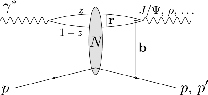
Fig. 1: Diffractive vector meson production in dipole picture.

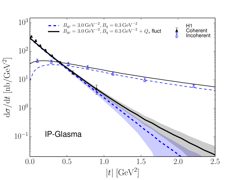
Fig. 2: Coherent and incoherent diffractive $J/\Psi$ production compared with the H1 data [12].

The scattering amplitude for diffractive vector meson production can be written as [5]

$$\mathcal{A}^{\gamma^{*}p\to Vp}_{T,L}({x_{\mathbb{P}}},Q^{2},\boldsymbol{\Delta})=2i\int\mathrm{d}^{2}{\mathbf{r}}\int\mathrm{d}^{2}{\mathbf{b}}\int\frac{\mathrm{d}z}{4\pi}(\Psi^{*}\Psi_{V})_{T,L}(Q^{2},{\mathbf{r}},z)e^{-i[{\mathbf{b}}-(1-z){\mathbf{r}}]\cdot\boldsymbol{\Delta}}N({\mathbf{b}},{\mathbf{r}},{x_{\mathbb{P}}}).$$ (1)

Here $Q^{2}$ is the virtuality of the photon, ${\mathbf{b}}$ impact parameter, ${\mathbf{r}}$ size of the quark-antiquark dipole and $z$ longitudinal momenum fraction of the photon carried by the quark. The transverse momentum of the vector meson $\boldsymbol{\Delta}\approx\sqrt{|t|}$ is the Fourier conjugate to ${\mathbf{b}}-(1-z){\mathbf{r}}$. This scattering probes the gluon distribution of the target at longitudinal momentum fraction ${x_{\mathbb{P}}}$. The dipole-proton amplitude $N$ is obtained as a trace of Wilson lines at positions ${\mathbf{b}}+{\mathbf{r}}/2$ and ${\mathbf{b}}-{\mathbf{r}}/2$. The interpretation of Eq. 1 is straightforward: first, the incoming virtual photon splits to a quark-antiquark dipole. This splitting is described by the virtual photon wave function $\Psi$. The dipole then scatters elastically off the proton, which is given in terms of the dipole scattering amplitude $N$. Finally, the quark-antiquark pair forms a vector meson according to the vector meson wave function $\Psi_{V}$. This is illustrated in Fig. 2.

The coherent diffractive cross section is obtained by averaging the scattering amplitude over different configurations of the proton, and then taking the square: $\frac{\mathrm{d}\sigma^{\gamma^{*}p\to Vp}}{\mathrm{d}t}=\frac{1}{16\pi}\left|\langle\mathcal{A}^{\gamma^{*}p\to Vp}({x_{\mathbb{P}}},Q^{2},\boldsymbol{\Delta})\rangle\right|^{2}.$ The incoherent cross section can be written as a variance [4] (see also Refs. [6, 7]):
$\frac{\mathrm{d}\sigma^{\gamma^{*}p\to Vp^{*}}}{\mathrm{d}t}=\frac{1}{16\pi}\left(\left\langle\left|\mathcal{A}^{\gamma^{*}p\to Vp}({x_{\mathbb{P}}},Q^{2},\boldsymbol{\Delta})\right|^{2}\right\rangle-\left|\langle\mathcal{A}^{\gamma^{*}p\to Vp}({x_{\mathbb{P}}},Q^{2},\boldsymbol{\Delta})\rangle\right|^{2}\right)\,.$

In the hydrodynamical simulations performed using Music [13, 14] we use the same second order transport parameters as in Ref. [15] and effective constant shear viscosity $\eta/s=0.2$. We also include bulk viscosity and use a temperature dependent $\zeta/s$ as in [15], which is essential in small systems to obtain average transverse momenta compatible with the LHC data. Before $\tau_{0}=0.2\,\mathrm{fm}/c$, when we start hydrodynamical evolution, the system is evolved by solving the classical Yang-Mills equations. The full energy momentum tensor $T^{\mu\nu}$ at $\tau_{0}$ is matched to the hydrodynamical phase. The hydrodynamic equations are evolved with a Lattice Equation of State s95p-v1 [16]. The switching temperature is set to $T_{\text{switch}}=155$ MeV, after which particles are sampled using the Cooper-Frye prescription and are allowed to propagate in the hadronic cascade model UrQMD [17]. For more details, see Ref. [10].

3 Results

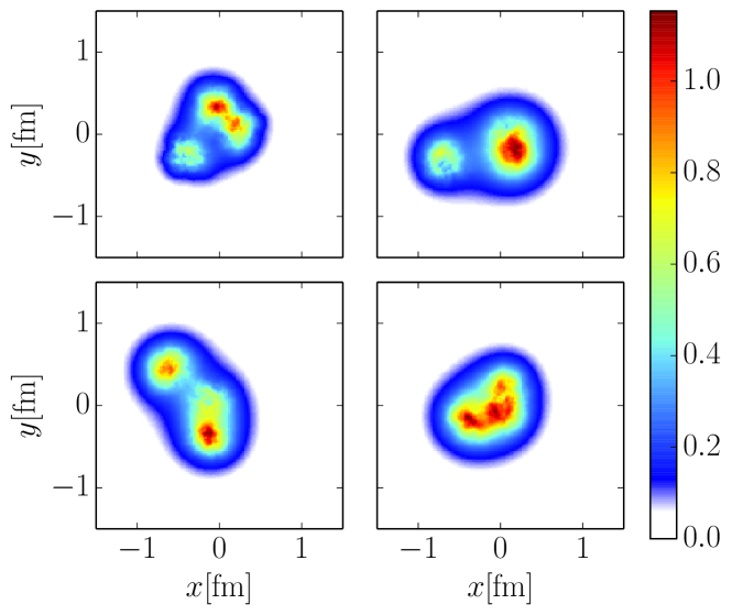
Fig. 3: Example of the proton density profiles at $x\approx 10^{-3}$. The quantity shown is $1-\mathrm{Re}\,\mathrm{Tr}V({\mathbf{x}})/N_{\mathrm{c}}$.

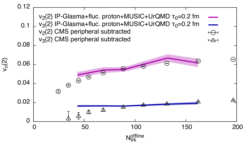
Fig. 4: Elliptic ($v_{2}$) and triangular ($v_{3}$) as a function of multiplicity compared to the CMS data [18].

First we constrain the amount of fluctuations by comparing with the H1 diffractive $J/\Psi$ photoproduction data [12]. The free parameters that describe the proton fluctuations, $B_{q}$ and $B_{qc}$ (see Sec. 2), are obtained by requiring a good simultaneous agreement with both coherent and incoherent diffractive cross sections. As these processes are separately sensitive to the average density profile and to the amount of fluctuations, this allows us to constrain both $B_{q}=0.3\ \textrm{GeV}^{-2}$ and $B_{qc}=3.0\ \textrm{GeV}^{-2}$. This corresponds to having large event-by-event fluctuations in the proton wave function. This is illustrated in Fig. 4, where we show $1-\mathrm{Re}\,\mathrm{Tr}V({\mathbf{x}})/N_{\mathrm{c}}$ which can be seen to be roughly proportional to the density of the proton.

Next, we take the fluctuating proton structure constrained previously and calculate elliptic and triangular flow in proton-lead collisions at $\sqrt{s_{NN}}=5.02$ TeV. The results are compared with the CMS data [18] in Fig. 4. In previous calculations within the same framework but without geometric fluctuations for the proton, the harmonic flow coefficients were largely underestimated [3]. This is in contrast to the results shown in Fig. 4, where a good agreement with the CMS data is obtained at large multiplicities. We also show in Ref. [10] that the HBT radii and mean transverse momenta are compatible with the measurements.

4 Conclusions

We have constrained the geometric fluctuations of the proton by comparing with the HERA coherent and incoherent diffractive vector meson production data. We find that in order to describe these measurements, large geometric fluctuations of the proton wave function are needed. Simulating proton-nucleus collisions using the fluctuating protons constrained by HERA data, we find a good description of the flow harmonics in high multiplicity events. In Ref. [19] the necessity of having large geometric fluctuations was also found to improve the description of the exclusive $J/\Psi$ production data in ultraperipheral heavy ion collisions at the LHC.

References

- [1] K. Dusling, W. Li, B. Schenke, Novel collective phenomena in high-energy proton–proton and proton–nucleus collisions, Int. J. Mod. Phys. E25 (2016) 1630002. arXiv:1509.07939, doi:10.1142/S0218301316300022.
- [2] B. Schenke, P. Tribedy, R. Venugopalan, Fluctuating Glasma initial conditions and flow in heavy ion collisions, Phys. Rev. Lett. 108 (2012) 252301. arXiv:1202.6646, doi:10.1103/PhysRevLett.108.252301.
- [3] B. Schenke, R. Venugopalan, Eccentric protons? Sensitivity of flow to system size and shape in p+p, p+Pb and Pb+Pb collisions, Phys. Rev. Lett. 113 (2014) 102301. arXiv:1405.3605, doi:10.1103/PhysRevLett.113.102301.
- [4] H. I. Miettinen, J. Pumplin, Diffraction Scattering and the Parton Structure of Hadrons, Phys. Rev. D18 (1978) 1696. doi:10.1103/PhysRevD.18.1696.
- [5] H. Kowalski, L. Motyka, G. Watt, Exclusive diffractive processes at HERA within the dipole picture, Phys. Rev. D74 (2006) 074016. arXiv:hep-ph/0606272, doi:10.1103/PhysRevD.74.074016.
- [6] L. Frankfurt, M. Strikman, D. Treleani, C. Weiss, Evidence for color fluctuations in the nucleon in high-energy scattering, Phys. Rev. Lett. 101 (2008) 202003. arXiv:0808.0182, doi:10.1103/PhysRevLett.101.202003.
- [7] T. Lappi, H. Mäntysaari, Incoherent diffractive -production in high energy nuclear DIS, Phys. Rev. C83 (2011) 065202. arXiv:1011.1988, doi:10.1103/PhysRevC.83.065202.
- [8] H. Mäntysaari, B. Schenke, Evidence of strong proton shape fluctuations from incoherent diffraction, Phys. Rev. Lett. 117 (2016) 052301. arXiv:1603.04349, doi:10.1103/PhysRevLett.117.052301.
- [9] H. Mäntysaari, B. Schenke, Revealing proton shape fluctuations with incoherent diffraction at high energy, Phys. Rev. D94 (3) (2016) 034042. arXiv:1607.01711, doi:10.1103/PhysRevD.94.034042.
- [10] H. Mäntysaari, B. Schenke, C. Shen, P. Tribedy, Imprints of fluctuating proton shapes on flow in proton-lead collisions at the LHCarXiv:1705.03177.
- [11] A. H. Rezaeian, M. Siddikov, M. Van de Klundert, R. Venugopalan, Analysis of combined HERA data in the Impact-Parameter dependent Saturation model, Phys. Rev. D87 (2013) 034002. arXiv:1212.2974, doi:10.1103/PhysRevD.87.034002.
- [12] C. Alexa, et al., Elastic and Proton-Dissociative Photoproduction of J Mesons at HERA, Eur. Phys. J. C73 (6) (2013) 2466. arXiv:1304.5162, doi:10.1140/epjc/s10052-013-2466-y.
- [13] B. Schenke, S. Jeon, C. Gale, (3+1)D hydrodynamic simulation of relativistic heavy-ion collisions, Phys. Rev. C82 (2010) 014903. arXiv:1004.1408, doi:10.1103/PhysRevC.82.014903.
- [14] B. Schenke, S. Jeon, C. Gale, Elliptic and triangular flow in event-by-event (3+1)D viscous hydrodynamics, Phys. Rev. Lett. 106 (2011) 042301. arXiv:1009.3244, doi:10.1103/PhysRevLett.106.042301.
- [15] S. Ryu, J. F. Paquet, C. Shen, G. S. Denicol, B. Schenke, S. Jeon, C. Gale, Importance of the Bulk Viscosity of QCD in Ultrarelativistic Heavy-Ion Collisions, Phys. Rev. Lett. 115 (13) (2015) 132301. arXiv:1502.01675, doi:10.1103/PhysRevLett.115.132301.
- [16] P. Huovinen, P. Petreczky, QCD Equation of State and Hadron Resonance Gas, Nucl. Phys. A837 (2010) 26–53. arXiv:0912.2541, doi:10.1016/j.nuclphysa.2010.02.015.
- [17] M. Bleicher, et al., Relativistic hadron hadron collisions in the ultrarelativistic quantum molecular dynamics model, J. Phys. G25 (1999) 1859–1896. arXiv:hep-ph/9909407, doi:10.1088/0954-3899/25/9/308.
- [18] S. Chatrchyan, et al., Multiplicity and transverse momentum dependence of two- and four-particle correlations in pPb and PbPb collisions, Phys. Lett. B724 (2013) 213–240. arXiv:1305.0609, doi:10.1016/j.physletb.2013.06.028.
- [19] H. Mäntysaari, B. Schenke, Probing subnucleon scale fluctuations in ultraperipheral heavy ion collisionsarXiv:1703.09256.