On Courant’s nodal domain property for linear combinations of eigenfunctions, Part I

Abstract.

According to Courant’s theorem, an eigenfunction associated with the $n$-th eigenvalue $\lambda_{n}$ has at most $n$ nodal domains. A footnote in the book of Courant and Hilbert, states that the same assertion is true for any linear combination of eigenfunctions associated with eigenvalues less than or equal to $\lambda_{n}$. We call this assertion the Extended Courant Property.

In this paper, we propose simple and explicit examples for which the extended Courant property is false: convex domains in $\mathbb{R}^{n}$ (hypercube and equilateral triangle), domains with cracks in $\mathbb{R}^{2}$, on the round sphere $\mathbb{S}^{2}$, and on a flat torus $\mathbb{T}^{2}$.

To appear in Documenta Mathematica.

1. Introduction

Let $\Omega\subset\mathbb{R}^{d}$ be a bounded open domain or, more generally, a compact Riemannian manifold with boundary.

Consider the eigenvalue problem

(1.1) $$\left\{\begin{array}[]{lll}-\Delta u&=\lambda\,u&\text{in\leavevmode\nobreak\ }\Omega\,,\\[5.0pt] \mathfrak{b}(u)&=0&\text{on\leavevmode\nobreak\ }\partial\Omega\,,\end{array}\right.$$

where $\mathfrak{b}(u)$ is some homogeneous boundary condition on $\partial\Omega$, so that we have a self-adjoint boundary value problem (including the empty condition if $\Omega$ is a closed manifold). For example, we can choose $\mathfrak{d}(u)=u|_{\partial\Omega}$ for the Dirichlet boundary condition, or $\mathfrak{n}(u)=\frac{\partial u}{\partial\nu}|_{\partial\Omega}$ for the Neumann boundary condition.

Call $H(\Omega,\mathfrak{b})$ the associated self-adjoint extension of $-\Delta$, and list its eigenvalues in nondecreasing order, counting multiplicities, and starting with the index $1$, as

(1.2) $$0\leq\lambda_{1}(\Omega,\mathfrak{b})<\lambda_{2}(\Omega,\mathfrak{b})\leq\lambda_{3}(\Omega,\mathfrak{b})\leq\cdots\,,$$

with an associated orthonormal basis of eigenfunctions $\{u_{j},j\geq 1\}$.

For any eigenvalue $\lambda$ of $(\Omega,\mathfrak{b})$, define the index

(1.3) $$\kappa(\Omega,\mathfrak{b},\lambda)=\min\{k\leavevmode\nobreak\ |\leavevmode\nobreak\ \lambda_{k}(\Omega,\mathfrak{b})=\lambda\}.$$

Notation.  If $\lambda$ is an eigenvalue of $(\Omega,\mathfrak{b})$, we denote by $\mathcal{E}(\Omega,\mathfrak{b},\lambda)$ the eigenspace associated with the eigenvalue $\lambda$.

We skip $\Omega$ or $\mathfrak{b}$ from the notations, whenever the context is clear.

Given a real continuous function $v$ on $\Omega$, define its nodal set

(1.4) $$\mathcal{Z}(v)=\overline{\left\{x\in\Omega\leavevmode\nobreak\ |\leavevmode\nobreak\ v(x)=0\right\}}\,,$$

and call $\beta_{0}(v)$ the number of connected components of $\Omega\setminus\mathcal{Z}(v)$ i.e., the number of nodal domains of $v$.

Theorem 1.1.

[Courant, 1923]
For any nonzero eigenfunction $u$ associated with $\lambda_{n}(\Omega,\mathfrak{b})$,

(1.5) $$\beta_{0}(u)\leq\kappa\big{(}\lambda_{n}(\Omega,\mathfrak{b})\big{)}\leq n\,.$$

Courant’s nodal domain theorem can be found in [13, Chap. V.6].

A footnote in [13, p. 454] (second footnote in the German original [12, p. 394]) indicates: Any linear combination of the first $n$ eigenfunctions divides the domain, by means of its nodes, into no more than $n$ subdomains. See the Göttingen dissertation of H. Herrmann, Beiträge zur Theorie der Eigenwerte und Eigenfunktionen, 1932.

For later reference, we write a precise statement. Given $\lambda\geq 0$, denote by $\mathcal{L}(\Omega,\mathfrak{b},\lambda)$ the space of linear combinations of eigenfunctions of $H(\Omega,\mathfrak{b})$ associated with eigenvalues less than or equal to $\lambda$,

(1.6) $$\mathcal{L}(\Omega,\mathfrak{b},\lambda)=\left\{\sum_{\lambda_{j}(\Omega,\mathfrak{b})\leq\lambda}c_{j}\,u_{j}\leavevmode\nobreak\ |\leavevmode\nobreak\ c_{j}\in\mathbb{R},u_{j}\in\mathcal{E}(\Omega,\mathfrak{b},\lambda_{j})\right\}\,.$$

Statement 1.2.

[Extended Courant Property]
Let $v\in\mathcal{L}\left(\lambda_{n}(\Omega,\mathfrak{b})\right)$ be any linear combination of eigenfunctions associated with the $n$ first eigenvalues of the eigenvalue problem (1.1). Then,

(1.7) $$\beta_{0}(v)\leq\kappa\big{(}\lambda_{n}(\Omega,\mathfrak{b})\big{)}\leq n\,.$$

We call both Statement 1.2, and Inequality (1.7), the Extended Courant Property, and refer to them as the $\mathrm{\textsc{ECP}}(\Omega)$, or as the $\mathrm{\textsc{ECP}}(\Omega,\mathfrak{b})$ to insist on the boundary condition $\mathfrak{b}$.

1.1. Known results and conjectures

We begin by recalling previously known results, and conjectures.

1.  Statement 1.2 is true for a finite interval, with either the Dirichlet or the Neumann boundary conditions, as well as for the periodic boundary conditions. In dimension $1$, one can actually replace the operator $\frac{d^{2}}{dx^{2}}$ by a general Sturm-Liouville operator $\frac{d}{dx}\left(K\frac{d}{dx}\right)+L$, where $K>0$ and $L$ are functions, see [7] and [10] for more details.

2.  In [1], see also [2, 22], Arnold points out that Statement 1.2 is particularly meaningful in relation to Hilbert’s 16th problem. Indeed, let $p$ be a homogeneous real polynomial in $(N+1)$ variables, of even degree $n$. When restricted to the sphere $\mathbb{S}^{N}$, or equivalently to the real projective space $\mathbb{R}P^{N}$, $p$ can be written as a sum of spherical harmonics of even degrees less than or equal to $n$, i.e., as a sum of eigenfunctions of the Laplace-Beltrami operator on $\mathbb{R}P^{N}$ equipped with the round metric $g_{0}$. Arnold observes that should $\mathrm{\textsc{ECP}}(\mathbb{R}P^{N},g_{0})$ be true, then the number of connected components of the complement to the algebraic hypersurface $V_{n}=p^{-1}(0)$ can be bounded from above by

$$\mathrm{dim}_{\mathbb{R}}H_{0}(\mathbb{R}P^{N}\!\setminus\!V_{n},\mathbb{R})\leq C_{N+n-2}^{N}+1\hskip 28.45274pt(1)$$

The estimate (1) is known to be true when $N=2$. It is known to be true when $N=3$ and $n=4$, and false when $N=3$ and $n\geq 6$, with counterexamples constructed by O. Viro [30].

It follows that $\mathrm{\textsc{ECP}}(\mathbb{R}P^{N},g_{0})$ is true for $N=2$, and false for $N=3$. Arnold also mentions that ECP is false for a generic metric $g$ on the sphere, but does not provide any precise statement, nor proof.

Remark. As mentioned above, $\mathrm{\textsc{ECP}}(\mathbb{R}P^{3},g_{0})$ is true when restricted to linear combinations of spherical harmonics of degree less than or equal to $4$. Given any $\lambda_{0}>0$, it is easy to construct a surface $(M,h)$ such that $\mathrm{\textsc{ECP}}(M,h)$ is true for linear combinations of eigenfunctions with eigenvalues less than or equal to $\lambda_{0}$. Indeed, let $(\mathbb{S}^{1},g_{a})$ be the circle with length $2a\pi$. The eigenvalues are the numbers $0$ (with multiplicity $1$), and ${n^{2}}/{a^{2}}$, for $n\geq 1$ (with multiplicity $2$). Consider the torus $(M,h_{a})=(\mathbb{S}^{1},g_{1})\times(\mathbb{S}^{1},g_{a})$. Fix some $\lambda_{0}>0$. Then, for $a$ small enough, the eigenfunctions of $(M,h_{a})$, associated with eigenvalues less than or equal to $\lambda_{0}$, correspond to eigenfunctions of the first factor $(\mathbb{S}^{1},g_{1})$, for which the extended Courant property is true.

Fix some $\lambda_{0}>0$. Using the Hopf fibration $\mathbb{S}^{3}\to\mathbb{S}^{2}$, and letting the length of the fiber tend to zero as in [11], one can find a metric $g_{\lambda_{0}}$ on $\mathbb{S}^{3}$, such that $\mathrm{\textsc{ECP}}(\mathbb{S}^{3},g_{\lambda_{0}})$ is true when restricted to linear combinations of eigenfunctions associated with eigenvalues less than or equal to $\lambda_{0}$.

3.  In [16], Gladwell and Zhu investigate Statement 1.2 (which they call the Courant-Herrmann conjecture) for domains in $\mathbb{R}^{N}$, with the Dirichlet boundary condition. For the Euclidean square $\mathcal{C}$, they show that $\mathrm{\textsc{ECP}}(\mathcal{C})$ is true when restricted to linear combinations of eigenfunctions associated with the first 13 eigenvalues. They make the conjectures that ECP is true for the square, for rectangles and, more generally for convex domains in $\mathbb{R}^{2}$.

They also give numerical evidence that the ECP is false for more complicated domains (rectangles with perturbed boundary). More precisely, they numerically determine the nodal sets of some linear combinations $c_{1}u_{1}+c_{2}u_{2}$ of the first two Dirichlet eigenfunctions in such domains, and conclude from the numerical computations that there exist domains for which the linear combinations $c_{1}u_{1}+c_{2}u_{2}$ have up to $5$ nodal domains. Finally, they also make the conjecture that given any integer $m\geq 2$, there exist a domain, and a linear combination $c_{1}u_{1}+c_{2}u_{2}$, with $m$ nodal domains.

Remark. Fix any $\lambda_{0}>0$. Then, for $a$ small enough, $\mathrm{\textsc{ECP}}([0,1]\times[0,a])$ is true when restricted to eigenfunctions associated with eigenvalues less than or equal to $\lambda_{0}$. The reasoning is similar to the one used in the preceding remark.

4.  Finally, we would like to point out that sums of eigenfunctions appear naturally in several contexts. (i)  Using the Faber-Krahn inequality, Pleijel improved Courant’s estimate for the Dirichlet Laplacian. In the case of the hypercube, an extension to the Neumann Laplacian could be achieved provided the extended Courant property be true, see [28]. (ii)  As far as their vanishing properties are concerned, eigenfunctions behave like polynomials with degree of the order of the square root of the eigenvalue. From this point of view, as pointed out in [21], it is natural to investigate the vanishing properties of sums of eigenfunctions as well. (iii)  What is the number of nodal domains of a “typical” eigenfunction? One can answer this question, in a probabilistic sense, when eigenspaces have large multiplicities. In a more general framework, one can consider sums of eigenfunctions. We refer to [27, 29] and the references in these papers. (iv)  A similar approach can be made in the framework of Hilbert’s 16th problem, see the paper [15] and its bibliography.

1.2. Main examples and organization of this paper

The purpose of the present paper is to provide simple counterexamples to the Extended Courant Property.

In this subsection, we briefly describe the main examples given in this paper. Each of them is directly motivated by a result or by a conjecture mentioned in the previous subsection.

1.  Let $\mathcal{C}_{n}:=[0,\pi]^{n}$ be the hypercube. In Section 2, we show that $\mathrm{\textsc{ECP}}(\mathcal{C}_{n},\mathfrak{d})$ is false for $n\geq 3$, and that $\mathrm{\textsc{ECP}}(\mathcal{C}_{n},\mathfrak{n})$ is false for $n\geq 4$. This provides convex counterexamples to the ECP in higher dimensions, for both the Dirichlet or the Neumann boundary conditions.

2.  Let $\mathcal{T}_{e}$ denote the equilateral triangle. In Section 3, we prove that $\mathrm{\textsc{ECP}}(\mathcal{T}_{e})$ is false for both the Dirichlet and the Neumann boundary conditions. This provides a convex counterexample to the ECP in dimension $2$, and therefore a counterexample to one of the conjectures in [16]. The description of the eigenvalues and eigenfunctions of the equilateral triangle is summarized in Appendix A.

Remark. By perturbing this example, one can show that there exists a family of smooth strictly convex domains $D_{a}$ in $\mathbb{R}^{2}$ such that the $\mathrm{\textsc{ECP}}(D_{a},\mathfrak{n})$ is false, see [8]. We refer to [10] for other counterexamples related to the equilateral triangle.

3.  In Section 4, we use cracks to perturb the rectangle, or the unit disk. We obtain non-convex, yet simply-connected domains of $\mathbb{R}^{2}$ which are counterexamples to the ECP. Similarly, in Sections 5 and 6, we use cracks to perturb a flat $2$-torus, or the round $2$-sphere, and obtain further counterexamples to the ECP.

In both cases, we can prescribe the number of nodal domains of the linear combination of eigenfunctions under consideration, thus answering a conjecture in [16].

Remark. By considering domains with cracks, we are able to provide a rigorous proof of the conjecture proposed in Gladwell and Zhu, based on numerical computations for some domains, and to extend it to the case of non-planar surfaces such as $\mathbb{T}^{2}$ and $\mathbb{S}^{2}$. These examples with cracks also contradict other natural conjectures (such as replacing the minimal labeling $\kappa(\lambda)$ in Statement 1.2, by a maximal labeling), for which the equilateral triangle is not a counterexample anymore.

4.  Finally, we would like to point out that some of our examples are relevant to the question of counting the number of connected components of the complement of a level line of the second Neumann eigenfunction, see [4].

Acknowledgements

The authors are very much indebted to Virginie Bonnaillie-Noël who produced some simulations and pictures at an early stage of their work on this subject. They thank the referee for his comments.

2. The hypercube

2.1. Preparation

Let $\mathcal{C}_{n}(\pi):=]0,\pi[^{\,n}$ be the hypercube of dimension $n$, with either the Dirichlet or the Neumann boundary condition on $\partial\mathcal{C}_{n}(\pi)$. A point in $\mathcal{C}_{n}(\pi)$ is denoted by $x=(x_{1},\ldots,x_{n})$.

A complete set of eigenfunctions of $-\Delta$ for $(\mathcal{C}_{n}(\pi),\mathfrak{d})$ is given by the functions

(2.1) $$\prod_{j=1}^{n}\sin(k_{j}\,x_{j})\,,\text{\leavevmode\nobreak\ with eigenvalue\leavevmode\nobreak\ }\sum_{j=1}^{n}k_{j}^{2},\text{\leavevmode\nobreak\ \leavevmode\nobreak\ for\leavevmode\nobreak\ }k_{j}\in\mathbb{N}\!\setminus\!\{0\}\,.$$

A complete set of eigenfunctions of $-\Delta$ for $(\mathcal{C}_{n}(\pi),\mathfrak{n})$ is given by the functions

(2.2) $$\prod_{j=1}^{n}\cos(k_{j}\,x_{j})\,,\text{\leavevmode\nobreak\ with eigenvalue\leavevmode\nobreak\ }\sum_{j=1}^{n}k_{j}^{2},\text{\leavevmode\nobreak\ \leavevmode\nobreak\ for\leavevmode\nobreak\ }k_{j}\in\mathbb{N}\,.$$

2.2. Hypercube with Dirichlet boundary condition

In this section, we make use of the classical Chebyshev polynomials $U_{k}(t),k\in\mathbb{N}$, defined by the relation,

$$\sin\left((k+1)t\right)=\sin(t)\,U_{k}\left(\cos(t)\right)\,,$$

and in particular,

$$U_{0}(t)=1,\leavevmode\nobreak\ \leavevmode\nobreak\ U_{1}(t)=2t,\leavevmode\nobreak\ \leavevmode\nobreak\ U_{2}(t)=4t^{2}-1\,.$$

The first Dirichlet eigenvalues of $\mathcal{C}_{n}(\pi)$ (as points in the spectrum) are listed in the following table, together with their multiplicities, and eigenfunctions.

Table 2.1. First Dirichlet eigenvalues of $\mathcal{C}_{n}(\pi)$

Eigenv.	Mult.	Eigenfunctions
$n$	$1$	$\phi_{1}(x):=\prod_{j=1}^{n}\sin(x_{j})$
$n+3$	$n$	$\phi_{1}(x)\,U_{1}\left(\cos(x_{i})\right)$, for $1\leq i\leq n$
$n+6$	$\frac{n(n-1)}{2}$	$\phi_{1}(x)\,U_{1}\left(\cos(x_{i})\right)\,U_{1}\left(\cos(x_{j})\right)$, for $1\leq i<j\leq n$
$n+8$	$n$	$\phi_{1}(x)\,U_{2}\left(\cos(x_{i})\right)$, for $1\leq i\leq n$

For the above eigenvalues, the index defined in (1.3) is given by,

(2.3) $$\kappa(n+3)=2,\leavevmode\nobreak\ \leavevmode\nobreak\ \kappa(n+6)=n+2,\leavevmode\nobreak\ \leavevmode\nobreak\ \kappa(n+8)=\frac{n(n+1)}{2}+2\,.$$

In order to study the nodal set of the above eigenfunctions or linear combinations thereof, we use the diffeomorphism

(2.4) $$(x_{1},\ldots,x_{n})\mapsto\left(\xi_{1}=\cos(x_{1}),\ldots\,,\xi_{n}=\cos(x_{n})\right)\,,$$

from $]0,\pi[^{n}$ onto $]-1,1[^{n}$, and factor out the function $\phi_{1}$ which does not vanish in the open hypercube. We consider the function

$$\Xi_{a}(\xi_{1},\ldots,\xi_{n})=\xi_{1}^{2}+\cdots+\xi_{n}^{2}-a$$

which corresponds to a linear combination $\Phi_{a}$ in

$$\mathcal{E}(\mathcal{C}_{n}(\pi),\mathfrak{d},n)\oplus\mathcal{E}(\mathcal{C}_{n}(\pi),\mathfrak{d},n+8).$$

Given some $a$, with $(n-1)<a<n$, the function $\Phi_{a}$ has $2^{n}+1$ nodal domains, see Figure 2.1 in dimension $3$. For $n\geq 3$, we have $2^{n}+1>\kappa(n+8)$. The function $\Phi_{a}$ therefore provides a counterexample to the ECP for the hypercube of dimension at least $3$, with Dirichlet boundary condition.

Proposition 2.1.

For $n\geq 3$, the $\mathrm{\textsc{ECP}}(\mathcal{C}_{n}(\pi),\mathfrak{d})$ is false.

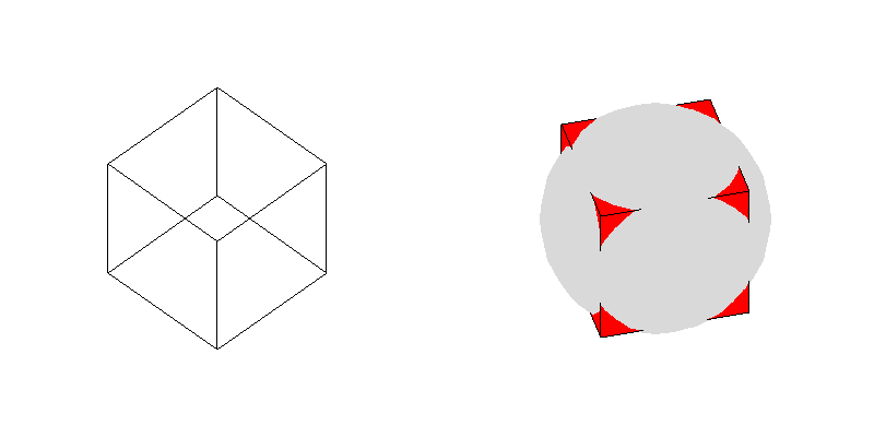
Figure 2.1. $3$-dimensional cube

Remark. An interesting feature of this example is that we get counterexamples to the ECP for linear combinations which involve eigenvalues with higher index when $n$ increases. This is also in contrast with the fact that, in dimension $3$, Courant’s nodal domain theorem is sharp only for $\delta_{1}$ and $\delta_{2}$, [19].

2.3. Hypercube with Neumann boundary condition

In this section, we make use of the classical Chebyshev polynomials $T_{k}(t),k\in\mathbb{N}$, defined by the relation,

$$\cos(kt)=T_{k}\left(\cos(t)\right),$$

and in particular,

$$T_{0}(t)=1\,,\leavevmode\nobreak\ \leavevmode\nobreak\ T_{1}(t)=t\,,\leavevmode\nobreak\ \leavevmode\nobreak\ T_{2}(t)=2t^{2}-1\,.$$

The first Neumann eigenvalues (as points in the spectrum) are listed in the following table, together with their multiplicities, and eigenfunctions.

Table 2.2. First Neumann eigenvalues of $\mathcal{C}_{n}(\pi)$

Eigenv.	Mult.	Eigenfunctions
$0$	$1$	$\psi_{1}(x):=1$
$1$	$n$	$\cos(x_{i})$, for $1\leq i\leq n$
$2$	$\frac{n(n-1)}{2}$	$\cos(x_{i})\,\cos(x_{j})$, for $1\leq i<j\leq n$
$3$	$\frac{n(n-1)(n-2)}{6}$	$\cos(x_{i})\,\cos(x_{j})\,\cos(x_{k})$, for $1\leq i<j<k\leq n$
$4$	$n+\binom{n}{4}$	$T_{2}\left(\cos(x_{i})\right)$, for $1\leq i\leq n$ and …

For these Neumann eigenvalues, the index defined in (1.3) is given by,

(2.5) $$\kappa(2)=n+2\,,\kappa(3)=\frac{n(n+1)}{2}+2\,,\kappa(4)=\frac{n(n^{2}+5)}{6}+2\,.$$

In order to study the nodal set of the above eigenfunctions or linear combinations thereof, we again use the diffeomorphism (2.4) and the function $\Xi_{a}$, which here corresponds to a linear combination $\Psi_{a}$ in $\mathcal{E}(\mathcal{C}_{n}(\pi),\mathfrak{n},0)\oplus\mathcal{E}(\mathcal{C}_{n}(\pi),\mathfrak{n},4)$. Given some $a$, with $(n-1)<a<n$, the function $\Psi_{a}$ has $2^{n}+1$ nodal domains. For $n\geq 4$, we have $2^{n}+1>\kappa(4)$. The function $\Psi_{a}$ therefore provides a counterexample to the ECP for the hypercube of dimension at least $4$, with Neumann boundary condition.

Proposition 2.2.

For $n\geq 4\,$, the $\mathrm{\textsc{ECP}}(\mathcal{C}_{n}(\pi),\mathfrak{n})$ is false.

2.4. A stability result for the cube

According to Subsection 2.2, the $\mathrm{\textsc{ECP}}(\mathcal{C}_{3}(\pi),\mathfrak{d})$ is false. Consider the rectangular parallelepiped $\mathcal{P}_{b}:=]0,b_{1}\pi[\times]0,b_{2}\pi[\times]0,b_{3}\pi[$, with $b=(b_{1},b_{2},b_{3}),\leavevmode\nobreak\ b_{i}>0$, and define the $a_{i}$ by $\sqrt{a_{i}}\,b_{i}=1$.

The Dirichlet eigenvalues $\delta_{i}(\mathcal{P}_{b})$ are the numbers $a_{1}k_{1}^{2}+a_{2}k_{2}^{2}+a_{3}k_{3}^{2}$, with associated eigenfunctions

(2.6) $$\prod_{i=1}^{3}\sin\left(k_{i}\sqrt{a_{i}}x_{i}\right),\leavevmode\nobreak\ \leavevmode\nobreak\ k_{i}\in\mathbb{N}\!\setminus\!\{0\}.$$

The eigenvalues are clearly continuous in the parameters $a_{i}$. For a generic triple $(a_{1},a_{2},a_{3})$ close enough to $(1,1,1)$, the first $12$ Dirichlet eigenvalues $\delta_{i}(\mathcal{P}_{b})$ are simple, and correspond to the same type of eigenfunctions as for the ordinary cube (same choices for the triples $(k_{1},k_{2},k_{3})$). This is for example the case if we take $a_{1}=1,a_{2}=1+\sqrt{2}/100$ and $a_{3}=1+\sqrt{3}/100$, see the numerical values in Table 2.3, where the Dirichlet eigenvalues are denoted $\delta_{i}$.

Table 2.3. Eigenvalues for $(\mathcal{C}_{3}(\pi),\mathfrak{d})$ and $(\mathcal{P}_{b},\mathfrak{d})$

Index	Triple	$\delta_{i}(\mathcal{C}_{3}(\pi))$	$\delta_{i}(\mathcal{P}_{b})$
$1$	$(1,1,1)$	$3$	$3.016$
$2$	$(2,1,1)$	$6$	$6.016$
$3$	$(1,2,1)$	$6$	$6.037$
$4$	$(1,1,2)$	$6$	$6.042$
$5$	$(2,2,1)$	$9$	$9.037$
$6$	$(2,1,2)$	$9$	$9.042$
$7$	$(1,2,2)$	$9$	$9.063$
$8$	$(3,1,1)$	$11$	$11.016$
$9$	$(1,3,1)$	$11$	$11.072$
$10$	$(1,1,3)$	$11$	$11.085$
$11$	$(2,2,2)$	$12$	$12.063$
$12$	$(3,2,1)$	$14$	$14.037$

One can then repeat the arguments of Subsection 2.2, and conclude that $\mathrm{\textsc{ECP}}(\mathcal{C}_{b},\mathfrak{d})$ is false, so that one has some kind of stability.

Proposition 2.3.

For $b:=(b_{1},b_{2},b_{3})$ close enough to $(1,1,1)$, the $\mathrm{\textsc{ECP}}(\mathcal{P}_{b},\mathfrak{d})$ is false.

Clearly, the same kind of argument can be applied in higher dimension, or for the Neumann boundary condition.

Remark. Note that the preceding examples still leave open the conjecture made by Gladwell and Zhu that ECP is true for convex domains in dimension $2$. A counterexample will be given in the next section.

3. The equilateral triangle

Let $\mathcal{T}_{e}$ denote the equilateral triangle with sides equal to $1$, Figure 3.1. The eigenvalues and eigenfunctions of $\mathcal{T}_{e}$, with either the Dirichlet or the Neumann condition on the boundary $\partial\mathcal{T}_{e}$, can be completely described, see [5, 26, 25], or [6]. We provide a summary in Appendix A.

In this section, we show that the equilateral triangle provides a counterexample to the Extended Courant Property for both the Dirichlet and the Neumann boundary conditions, contradicting the conjecture of Gladwell and Zhu in dimension $2$.

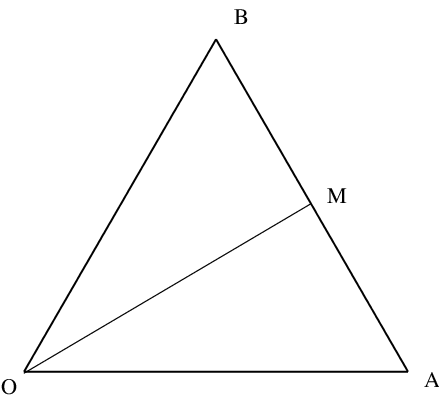
Figure 3.1. Equilateral triangle $\mathcal{T}_{e}=[OAB]$

3.1. Neumann boundary condition

The sequence of Neumann eigenvalues of the equilateral triangle $\mathcal{T}_{e}$ begins as follows,

(3.1) $$0=\lambda_{1}(\mathcal{T}_{e},\mathfrak{n})<\frac{16\pi^{2}}{9}=\lambda_{2}(\mathcal{T}_{e},\mathfrak{n})=\lambda_{3}(\mathcal{T}_{e},\mathfrak{n})<\lambda_{4}(\mathcal{T}_{e},\mathfrak{n})\,.$$

The second eigenspace has dimension $2$, and contains one eigenfunction $\varphi^{\mathfrak{n}}_{2}$ which is invariant under the mirror symmetry with respect to the median $OM$, and another eigenfunction $\varphi^{\mathfrak{n}}_{3}$ which is anti-invariant under the same mirror symmetry, see Appendix A.

More precisely, according to (A.21), the function $\varphi^{\mathfrak{n}}_{2}(x,y)$ can be chosen to be,

(3.2) $$\left\{\begin{array}[]{l}\begin{array}[]{ll}\varphi^{\mathfrak{n}}_{2}(x,y)=&\cos(\frac{4\pi}{3}x)+\cos(\frac{2\pi}{3}(-x+\sqrt{3}y))\\[3.0pt] &+\cos(\frac{2\pi}{3}(x+\sqrt{3}y))\,,\end{array}\end{array}\right.$$

or, more simply,

(3.3) $$\varphi^{\mathfrak{n}}_{2}(x,y)=2\cos\left(\frac{2\pi x}{3}\right)\left(\cos\left(\frac{2\pi x}{3}\right)+\cos\left(\frac{2\pi y}{\sqrt{3}}\right)\right)-1\,.$$

The set $\{\varphi^{\mathfrak{n}}_{2}+1=0\}$ consists of the two line segments $\{x=\frac{3}{4}\}\cap\mathcal{T}_{e}$ and $\{x+\sqrt{3}y=\frac{3}{2}\}\cap\mathcal{T}_{e}$, which meet at the point $(\frac{3}{4},\frac{\sqrt{3}}{4})$ on $\partial\mathcal{T}_{e}$.

The sets $\{\varphi^{\mathfrak{n}}_{2}+a=0\}$, with $a\in\{0\,;1-\varepsilon\,;1\,;1+\varepsilon\}$, and small positive $\varepsilon$, are shown in Figure 3.2. When $a$ varies from $1-\varepsilon$ to $1+\varepsilon$, the number of nodal domains of $\varphi^{\mathfrak{n}}_{2}+a$ in $\mathcal{T}_{e}$ jumps from $2$ to $3$, with the jump occurring for $a=1$.

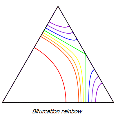
Figure 3.2. Level sets $\{\varphi^{\mathfrak{n}}_{2}+a=0\}$ for ${a\in\{0\,;\,0.7\,;\,0.8\,;\,0.9\,;\,1\,;\,1.1\,;\,1.2\,;\,1.3\}}$

It follows that $\varphi^{\mathfrak{n}}_{2}+a=0$, for $1\leq a\leq 1.1$, provides a counterexample to the Extended Courant Property for the equilateral triangle with Neumann boundary condition.

Proposition 3.1.

The $\mathrm{\textsc{ECP}}(\mathcal{T}_{e},\mathfrak{n})$ is false.

Remark. The eigenfunction $\varphi^{\mathfrak{n}}_{2}$ restricted to the hemiequilateral triangle is the second Neumann eigenfunction of $\mathcal{T}_{h}=[OAM]$. The restriction of $\varphi^{\mathfrak{n}}_{3}$ to the hemiequilateral triangle is an eigenfunction of $\mathcal{T}_{h}$ with mixed boundary condition (Dirichlet on $OM$ and Neumann on the other sides).

3.2. Dirichlet boundary condition

The sequence of Dirichlet eigenvalues of the equilateral triangle $\mathcal{T}_{e}$ begins as follows,

(3.4) $$\lambda_{1}(\mathcal{T}_{e},\mathfrak{d})=\frac{16\pi^{2}}{3}<\lambda_{2}(\mathcal{T}_{e},\mathfrak{d})=\lambda_{3}(\mathcal{T}_{e},\mathfrak{d})=\frac{112\pi^{2}}{9}<\lambda_{4}(\mathcal{T}_{e},\mathfrak{d}).$$

More precisely, according to (A.23), the function $\varphi^{\mathfrak{d}}_{1}(x,y)$ can be chosen to be,

(3.5) $$\begin{array}[]{ll}\varphi^{\mathfrak{d}}_{1}(x,y)&=-8\,\sin\frac{2\pi y}{\sqrt{3}}\,\sin\pi(x+\frac{y}{\sqrt{3}})\,\sin\pi(x-\frac{y}{\sqrt{3}})\,,\end{array}$$

which shows that $\varphi^{\mathfrak{d}}_{1}$ does not vanish inside $\mathcal{T}_{e}\,$.

The second eigenvalue has multiplicity $2$. It admits one eigenfunction, $\varphi^{\mathfrak{d}}_{2}$, which is symmetric with respect to the median $OM$, and given in (A.25), and another one, $\varphi^{\mathfrak{d}}_{3}$, which is anti-symmetric.

We now consider the linear combination $\varphi^{\mathfrak{d}}_{2}+a\,\varphi^{\mathfrak{d}}_{1}$, with $a$ close to $1$. The following lemma is the key for reducing the question to the previous analysis.

Lemma 3.2.

With the above notation, the following identity holds,

$$\varphi^{\mathfrak{d}}_{2}=\varphi^{\mathfrak{d}}_{1}\varphi^{\mathfrak{n}}_{2}\,.$$

Proof.

We express the above eigenfunctions in terms of $X:=\cos\frac{2\pi}{3}x$ and $Y:=\cos\frac{2\pi}{\sqrt{3}}y$.

First we observe from (3.3) that

$$\varphi^{\mathfrak{n}}_{2}(x,y)=2X(X+Y)-1\,.$$

Secondly, we have from (3.5)

$$\varphi^{\mathfrak{d}}_{1}(x,y)=2\sin\frac{2\pi y}{\sqrt{3}}\,(8X^{3}-6X-2Y)\,.$$

Finally, it remains to compute $\varphi^{\mathfrak{d}}_{2}$. We start from (A.25), and first factorize $\sin\frac{2\pi y}{\sqrt{3}}$ in each line. More precisely, we write,

(3.6) $$\begin{array}[]{ll}\sin\frac{2\pi}{3}(5x+\sqrt{3}y)-\sin\frac{2\pi}{3}(5x-\sqrt{3}y)=2\sin(\frac{2\pi y}{\sqrt{3}})\cos(5\frac{2\pi x}{3})\,,\\[5.0pt] \sin\frac{2\pi}{3}(x-3\sqrt{3}y)-\sin\frac{2\pi}{3}(x+3\sqrt{3}y)=-2\sin(3\frac{2\pi y}{\sqrt{3}})\cos(\frac{2\pi x}{3})\,,\\[5.0pt] \sin\frac{4\pi}{3}(2x+\sqrt{3}y)-\sin\frac{4\pi}{3}(2x-\sqrt{3}y)=2\sin(2\frac{2\pi y}{\sqrt{3}})\cos(4\frac{2\pi x}{3})\,.\end{array}$$

We now use the classical Chebyshev polynomials $T_{n},U_{n}$, and the relations $\cos(n\theta)=T_{n}(\cos\theta)$ and $\sin(n+1)\theta=\sin(\theta)\,U_{n}(\cos\theta)$.

This gives,

$$\begin{array}[]{ll}\varphi^{\mathfrak{d}}_{2}&=2\sin\frac{2\pi y}{\sqrt{3}}\Big{(}T_{5}(X)-XU_{2}(Y)+T_{4}(X)U_{1}(Y)\Big{)}\\[8.0pt] &=:2\sin\frac{2\pi y}{\sqrt{3}}\,Q(X,Y)\,.\end{array}$$

We find that

$$Q(X,Y)=16X^{5}-20X^{3}+6X+2Y(8X^{4}-8X^{2}+1)-4XY^{2}\,,$$

and it turns out that the polynomial $Q(X,Y)$ can be factorized as

$$Q(X,Y)=\big{(}2X(X+Y)-1\big{)}\,(8X^{3}-6X-2Y)\,,$$

so that $\varphi^{\mathfrak{d}}_{2}=\varphi^{\mathfrak{d}}_{1}\varphi^{\mathfrak{n}}_{2}$.

In the above computation, we have used the relations,

$$T_{4}(X)=8X^{4}-8X^{2}+1\,,\,T_{5}(X)=16X^{5}-20X^{3}+5X\,,\,$$

and

$$U_{1}(Y)=2Y\,,\,U_{2}(Y)=4Y^{2}-1\,.$$

∎

Observing that

$$\varphi^{\mathfrak{d}}_{2}+a\,\varphi^{\mathfrak{d}}_{1}=\varphi_{1}^{\mathfrak{d}}(\varphi^{\mathfrak{n}}_{2}+a)\,,$$

we deduce immediately from the Neumann result that the function $\varphi^{\mathfrak{d}}_{2}+a\,\varphi^{\mathfrak{d}}_{1}$, for $1\leq a\leq 1.1$, provides a counterexample to the Extended Courant Property for the equilateral triangle with the Dirichlet boundary condition.

Proposition 3.3.

The $\mathrm{\textsc{ECP}}(\mathcal{T}_{e},\mathfrak{d})$ is false.

Remark 3.4.

Lemma 3.2 is quite puzzling. However, other such identities do exist. Indeed, consider the square $\mathcal{C}_{2}(\pi)$. The first eigenfunction has the form

$$(x,y)\mapsto\alpha_{0}\sin x\sin y\,,$$

with $\alpha_{0}\neq 0\,$, and the second eigenfunctions take the form

$$(x,y)\mapsto\alpha\sin 2x\sin y+\beta\sin 2y\sin x\,,$$

with $|\alpha|+|\beta|\neq 0\,$. We can then observe that

$$\alpha\sin 2x\sin y+\beta\sin 2y\sin x=2\sin x\sin y\,(\alpha\cos x+\beta\cos y)\,,$$

and that $\alpha\cos x+\beta\cos y$ is a Neumann eigenfunction of the square. For $\mathcal{C}_{2}(\pi)$, more general relations between Dirichlet and Neumann eigenfunctions follow from the identity $2T_{n}=U_{n}-U_{n-2}$ between Chebyshev polynomials.
One can also prove the identity $\varphi_{2}^{\mathfrak{d}}=a\,\varphi_{1}^{\mathfrak{d}}\,\varphi_{2}^{\mathfrak{n}}$ between the eigenfunctions of the right isosceles triangle (for some constant $a$ depending on the normalization of eigenfunctions).

4. Rectangle with a crack

Let $\mathcal{R}$ be the rectangle $]0,4\pi[\times]0,2\pi[$. For $0<a\leq 1$, let $C_{a}:=]0,a]\times\{\pi\}$ and $\mathcal{R}_{a}:=\mathcal{R}\setminus C_{a}$. In this section, we only consider the Neumann boundary condition on $C_{a}$, and either the Dirichlet or the Neumann boundary condition on $\partial\mathcal{R}$. The setting is the one described in [14, Section 8].

We call

(4.1) $$\left\{\begin{array}[]{l}0<\delta_{1}(0)<\delta_{2}(0)\leq\delta_{3}(0)\leq\cdots\\ \text{resp.}\\[5.0pt] 0=\nu_{1}(0)<\nu_{2}(0)\leq\nu_{3}(0)\leq\cdots\end{array}\right.$$

the eigenvalues of $-\Delta$ in $\mathcal{R}$, with the Dirichlet (resp. the Neumann) boundary condition on $\partial\mathcal{R}$. They are given by the numbers $\frac{m^{2}}{16}+\frac{n^{2}}{4}$, for pairs $(m,n)$ of positive integers for the Dirichlet problem (resp. for pairs of non-negative integers for the Neumann problem). Corresponding eigenfunctions are products of sines (Dirichlet) or cosines (Neumann). The eigenvalues are arranged in non-decreasing order, counting multiplicities.

Similarly, call

(4.2) $$\left\{\begin{array}[]{l}0<\delta_{1}(a)<\delta_{2}(a)\leq\delta_{3}(a)\leq\cdots\\ \text{resp.}\\[5.0pt] 0=\nu_{1}(a)<\nu_{2}(a)\leq\nu_{3}(a)\leq\cdots\end{array}\right.$$

the eigenvalues of $-\Delta$ in $\mathcal{R}_{a}$, with the Dirichlet (resp. the Neumann) boundary condition on $\partial\mathcal{R}$, and the Neumann boundary condition on $C_{a}$.

The first three Dirichlet (resp. Neumann) eigenvalues for the rectangle $\mathcal{R}$ are as follows.

(4.3) $$\begin{array}[]{|c|c|c|c|}\hline\cr\text{Eigenvalue}&\text{Value}&\text{Pairs}&\text{Dirichlet eigenfunctions}\\[5.0pt] \hline\cr\delta_{1}(0)&\frac{5}{16}&(1,1)&\phi_{1}(x,y)=\sin(\frac{x}{4})\,\sin(\frac{y}{2})\\[5.0pt] \hline\cr\delta_{2}(0)&\frac{1}{2}&(2,1)&\phi_{2}(x,y)=\sin(\frac{x}{2})\,\sin(\frac{y}{2})\\[5.0pt] \hline\cr\delta_{3}(0)&\frac{13}{16}&(3,1)&\phi_{3}(x,y)=\sin(\frac{3x}{4})\,\sin(\frac{y}{2})\\[5.0pt] \hline\cr\end{array}$$

(4.4) $$\begin{array}[]{|c|c|c|c|}\hline\cr\text{Eigenvalue}&\text{Value}&\text{Pairs}&\text{Neumann eigenfunctions}\\[5.0pt] \hline\cr\nu_{1}(0)&0&(0,0)&\psi_{1}(x,y)=1\\[5.0pt] \hline\cr\nu_{2}(0)&\frac{1}{16}&(1,0)&\psi_{2}(x,y)=\cos(\frac{x}{4})\\[5.0pt] \hline\cr\nu_{3}(0)&&(0,1)&\psi_{3}(x,y)=\cos(\frac{y}{2})\\[5.0pt] \nu_{4}(0)&\frac{1}{4}&(2,0)&\psi_{4}(x,y)=\cos(\frac{x}{2})\\[5.0pt] \hline\cr\end{array}$$

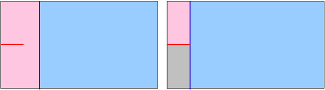
Figure 4.1. Rectangle with a crack (Neumann condition)

We summarize [14], Propositions (8.5), (8.7), (9.5) and (9.9), into the following theorem.

Theorem 4.1 (Dauge-Helffer).

With the above notation, the following properties hold.

1. For $i\geq 1$, the functions $[0,1]\ni a\mapsto\delta_{i}(a)$, resp. $[0,1]\ni a\mapsto\nu_{i}(a)$, are non-increasing.

2. For $i\geq 1$, the functions $]0,1[\ni a\mapsto\delta_{i}(a)$, resp. $]0,1[\ni a\mapsto\nu_{i}(a)$, are continuous.

3. For $i\geq 1$, $\lim_{a\to 0+}\delta_{i}(a)=\delta_{i}(0)$ and $\lim_{a\to 0+}\nu_{i}(a)=\nu_{i}(0)$.

It follows that for $a$ positive, small enough, we have

(4.5) $$\left\{\begin{array}[]{l}0<\delta_{1}(a)\leq\delta_{1}(0)<\delta_{2}(a)\leq\delta_{2}(0)<\delta_{3}(a)\leq\delta_{3}(0)\,,\text{and}\\[5.0pt] 0=\nu_{1}(a)=\nu_{1}(0)<\nu_{2}(a)\leq\nu_{2}(0)<\nu_{3}(a)\leq\nu_{4}(a)\leq\nu_{3}(0)\,.\end{array}\right.$$

Observe that for $i=1$ and $2$, $\frac{\partial\phi_{i}}{\partial y}(x,\pi)=0$ and $\frac{\partial\psi_{i}}{\partial y}(x,y)=0$. It follows that for $a$ small enough, the functions $\phi_{1}$ and $\phi_{2}$ (resp. the functions $\psi_{1}$ and $\psi_{2}$) are the first two eigenfunctions for $\mathcal{R}_{a}$ with the Dirichlet (resp. Neumann) boundary condition on $\partial\mathcal{R}$, and the Neumann boundary condition on $C_{a}$, with associated eigenvalues $\frac{5}{16}$ and $\frac{1}{2}$ (resp. $0$ and $\frac{1}{16}$).

We have

$$\alpha\phi_{1}(x,y)+\beta\phi_{2}(x,y)=\sin(\frac{x}{4})\,\sin(\frac{y}{2})\,\left(\alpha+2\beta\cos(\frac{x}{4})\right),$$

and

$$\alpha\psi_{1}(x,y)+\beta\psi_{2}(x,y)=\alpha+\beta\cos(\frac{x}{4}).$$

We can choose the coefficients $\alpha,\beta$ in such a way that these linear combinations of the first two eigenfunctions have two (Figure 4.1 left) or three (Figure 4.1 right) nodal domains in $\mathcal{R}_{a}\,$.

Proposition 4.2.

The $\mathrm{\textsc{ECP}}(\mathcal{R}_{a})$ is false with the Neumann condition on $C_{a}$, and either the Dirichlet or the Neumann condition on $\partial\mathcal{R}$.

Remark 4.3.

In the Neumann case, we can introduce several cracks $\{(x,b_{j})\leavevmode\nobreak\ |\leavevmode\nobreak\ 0<x<a_{j}\}_{j=1}^{k}$ in such a way that for any $d\in\{2,3,\ldots k+2\}$ there exists a linear combination of $1$ and $\cos(\frac{x}{4})$ with $d$ nodal domains.

Remark 4.4.

Numerical simulations, kindly provided by Virginie Bonnaillie-Noël, indicate that the Extended Courant Property does not hold for a rectangle with a crack, with the Dirichlet boundary condition on both the boundary of the rectangle, and the crack, [9]. Dirichlet cracks appear in another context in [17] (see also references therein)

Remark 4.5.

It is easy to make an analogous construction for the unit disk (Neumann case) with radial cracks. As computed for example in [20] (Subsection 3.4), the second radial eigenfunction has labelling $6$ ($\lambda_{6}\approx 14,68$), and we can introduce six radial cracks to obtain a combination of the two first radial Neumann eigenfunctions with seven nodal domains, see Figure 4.2.

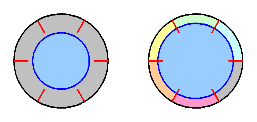
Figure 4.2. Disk with cracks, Neumann condition

5. The rectangular flat torus with cracks

Consider the flat torus $\mathbb{T}:=\mathbb{R}^{2}/\left(4\pi\mathbb{Z}\oplus 2\pi Z\right)$. Arrange the eigenvalues in nondecreasing order,

(5.1) $$\lambda_{1}(0)<\lambda_{2}(0)\leq\lambda_{3}(0)\leq\cdots$$

The eigenvalues are given by the numbers $\frac{m^{2}}{4}+n^{2}$ for $(m,n)$ pairs of integers, with associated complex eigenfunctions

(5.2) $$\exp(im\frac{x}{2})\,\exp(iny)$$

or equivalently, with real eigenfunctions

(5.3) $$\begin{array}[]{l}\cos(m\frac{x}{2})\,\cos(ny),\,\cos(m\frac{x}{2})\,\sin(ny),\\[5.0pt] \sin(m\frac{x}{2})\,\cos(ny),\,\sin(m\frac{x}{2})\,\sin(ny),\end{array}$$

where $m,n$ are non-negative integers. Accordingly, the first eigenpairs of $\mathcal{T}$ are as follows.

(5.4) $$\begin{array}[]{|c|c|c|c|}\hline\cr\text{Eigenvalue}&\text{Value}&\text{Pairs}&\text{Eigenfunctions}\\[5.0pt] \hline\cr\lambda_{1}(0)&0&(0,0)&\omega_{1}(x,y)=1\\[5.0pt] \hline\cr\lambda_{2}(0)&&&\omega_{2}(x,y)=\cos(\frac{x}{2})\\[5.0pt] \lambda_{3}(0)&\frac{1}{4}&(1,0)&\omega_{2}(x,y)=\sin(\frac{x}{2})\\[5.0pt] \hline\cr\lambda_{4}(0)&&&\omega_{3}(x,y)=\cos(y)\\[5.0pt] \lambda_{5}(0)&1&(0,1)&\omega_{4}(x,y)=\sin(y)\\[5.0pt] \hline\cr\end{array}$$

A typical linear combination of the first three eigenfunctions is of the form $\alpha+\beta\,\sin(\frac{x}{2}-\theta)$

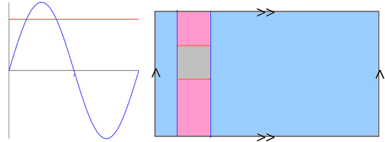
Figure 5.1. Flat torus with two cracks

Take the torus $\mathbb{T}$, and perform two (or more) cracks parallel to the $x$ axis, and with the same length $a$. Call $\mathbb{T}_{a}$ the torus with cracks, see Figure 5.1, and choose the Neumann boundary condition on the cracks. For $a$ small enough, the first three eigenfunctions of the torus $\mathbb{T}$ remain eigenfunctions of the torus with cracks, $\mathbb{T}_{a}$, with the same $\kappa(\mathbb{T}_{a},3)=2$. The proof is the same as in [14]. We can choose the length $a$ such that the nodal set of $\alpha+\beta\,\sin(\frac{x}{2}-\theta)$ and the two cracks determine three nodal domains.

Proposition 5.1.

The Extended Courant Property is false for the flat torus with cracks (Neumann condition on the cracks).

6. Sphere $\mathbb{S}^{2}$ with cracks

According to [24, Theorem 1, p. 305], the ECP is true on the round sphere $\mathbb{S}^{2}$ for sums of spherical harmonics of even (resp. of odd) degree. We consider the geodesic lines $z\mapsto(\sqrt{1-z^{2}}\cos\theta_{i},\sqrt{1-z^{2}}\sin\theta_{i},z)$ through the north pole $(0,0,1)$, with distinct $\theta_{i}\in[0,\pi[$. For example, removing the geodesic segments $\theta_{0}=0$ and $\theta_{2}=\frac{\pi}{2}$ with $1-z\leq a\leq 1$, we obtain a sphere $\mathbb{S}^{2}_{a}$ with a crack in the form of a cross. We choose the Neumann boundary condition on the crack.

We can then easily produce a function, in the space generated by the two first eigenspaces of the sphere with a crack, having five nodal domains.

The first eigenvalue of $\mathbb{S}^{2}$ is $\lambda_{1}(0)=0$, with corresponding eigenspace of dimension $1$, generated by the function $1$. The next eigenvalues of $\mathbb{S}^{2}$ are $\lambda_{2}(0)=\lambda_{3}(0)=\lambda_{4}(0)=2$ with associated eigenspace of dimension $3$, generated by the functions $x,y,z$. The following eigenvalues of $\mathbb{S}^{2}$ are larger than or equal to $6$.

As in [14], the eigenvalues of $\mathbb{S}^{2}_{a}$ (with Neumann condition on the crack) are non-increasing in $a$, and continuous to the right at $a=0$. More precisely

(6.1) $$\left\{\begin{array}[]{l}0=\lambda_{1}(a)<\lambda_{2}(a)\leq\lambda_{3}(a)\leq\lambda_{4}(a)\leq 2<\lambda_{5}(a)\leq 6\,,\\[5.0pt] \lim_{a\to 0+}\lambda_{i}(a)=2\text{\leavevmode\nobreak\ for\leavevmode\nobreak\ }i=2,3,4,\\[5.0pt] \lim_{a\to 0+}\lambda_{5}(a)=6\,.\end{array}\right.$$

The function $z$ is also an eigenfunction of $\mathbb{S}^{2}_{a}$ with eigenvalue $2$. It follows from (6.1) that for $a$ small enough, $\lambda_{4}(a)=2$, with eigenfunction $z$. For $0<b<a$, the linear combination $z-b$ has five nodal domains in $\mathbb{S}^{2}_{a}$, see Figure 6.1 in spherical coordinates.

Proposition 6.1.

The Extended Courant Property is false for the round $2$-sphere with cracks (Neumann condition on the cracks).

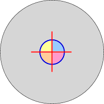
Figure 6.1. Sphere with crack, five nodal domains

Remark 6.2.

(1) Removing more geodesic segments around the north pole, we can obtain a linear combination $z-b$ with as many nodal domains as we want.
(2) The sphere with cracks, and Dirichlet condition on the cracks, has been considered for another purpose in [18].

Appendix A Eigenvalues of the equilateral triangle

In this appendix, we recall the description of the eigenvalues of the equilateral triangle. For the reader’s convenience, we retain the notation of [6, Section 2].

A.1. General formulas

Let $\mathbb{E}^{2}$ be the Euclidean plane with the canonical orthonormal basis $\{e_{1}=(1,0),e_{2}=(0,1)\}$, scalar product $\langle\cdot,\cdot\rangle$ and associated norm $|\cdot|$.

Consider the vectors

(A.1) $$\alpha_{1}=(1,-\frac{1}{\sqrt{3}}),\alpha_{2}=(0,\frac{2}{\sqrt{3}}),\alpha_{3}=(1,\frac{1}{\sqrt{3}})=\alpha_{1}+\alpha_{2}\,,$$

and

(A.2) $$\alpha{}^{\vee}_{1}=(\frac{3}{2},-\frac{\sqrt{3}}{2}),\alpha{}^{\vee}_{2}=(0,\sqrt{3}),\alpha{}^{\vee}_{3}=(\frac{3}{2},\frac{\sqrt{3}}{2})=\alpha{}^{\vee}_{1}+\alpha{}^{\vee}_{2}\,.$$

Then

(A.3) $$\alpha{}^{\vee}_{i}=\frac{3}{2}\alpha_{i},|\alpha_{i}|^{2}=\frac{4}{3},|\alpha{}^{\vee}_{i}|^{2}=3.$$

Define the mirror symmetries

(A.4) $$s_{i}(x)=x-2\frac{\langle x,\alpha_{i}\rangle}{\langle\alpha_{i},\alpha_{i}\rangle}\alpha_{i}=x-\frac{2}{3}\langle x,\alpha{}^{\vee}_{i}\rangle\alpha{}^{\vee}_{i}\,,$$

whose axes are the lines

(A.5) $$L_{i}=\{x\in\mathbb{E}^{2}\leavevmode\nobreak\ |\leavevmode\nobreak\ \langle x,\alpha_{i}\rangle=0\}.$$

Let $W$ be the group generated by these mirror symmetries. Then,

(A.6) $$W=\{1,s_{1},s_{2},s_{3},s_{1}\circ s_{2},s_{1}\circ s_{1}\}\,,$$

where $s_{1}\circ s_{2}$ (resp. $s_{2}\circ s_{1}$) is the rotation with center the origin and angle $\frac{2\pi}{3}$ (resp. $-\frac{2\pi}{3}$).

Remark. The above vectors are related to the root system $A_{2}$ and $W$ is the Weyl group of this root system.

Let

(A.7) $$\Gamma=\mathbb{Z}\alpha{}^{\vee}_{1}\oplus\mathbb{Z}\alpha{}^{\vee}_{2}$$

be the (equilateral) lattice. The set

(A.8) $$\mathcal{D}_{\Gamma}=\{s\alpha{}^{\vee}_{1}+t\alpha{}^{\vee}_{2}\leavevmode\nobreak\ |\leavevmode\nobreak\ 0\leq s,t\leq 1\}$$

is a fundamental domain for the action of $\Gamma$ on $\mathbb{E}^{2}$. Another fundamental domain is the closure of the open hexagon (see Figure A.1)

(A.9) $$\mathcal{H}=[A,B,C,D,E,F]\,,$$

whose vertices are given by

(A.10) $$\left\{\begin{array}[]{l}A=(1,0);B=(\frac{1}{2},\frac{\sqrt{3}}{2});C=(-\frac{1}{2},\frac{\sqrt{3}}{2});\\[5.0pt] D=(-1,0);E=(-\frac{1}{2},-\frac{\sqrt{3}}{2});F=(\frac{1}{2},-\frac{\sqrt{3}}{2})\,.\end{array}\right.$$

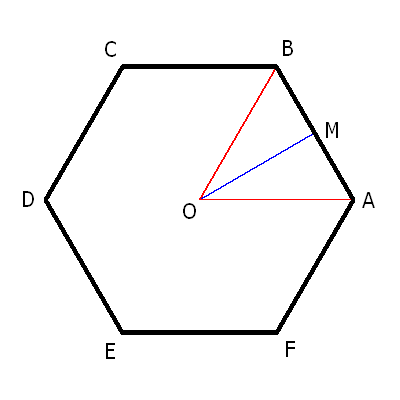
Figure A.1. The hexagon $\mathcal{H}$

Call $\mathcal{T}_{e}$ the equilateral triangle

(A.11) $$\mathcal{T}_{e}=[O,A,B]\,,$$

where $O=(0,0)$.

Let $\Gamma^{*}$ be the dual lattice of the lattice $\Gamma$, defined by

(A.12) $$\Gamma^{*}=\{x\in\mathbb{E}^{2}\leavevmode\nobreak\ |\leavevmode\nobreak\ \forall\gamma\in\Gamma,\langle x,\gamma\rangle\in\mathbb{Z}\}\,.$$

Then,

(A.13) $$\left\{\begin{array}[]{l}\Gamma^{*}=\mathbb{Z}\varpi_{1}\oplus\mathbb{Z}\varpi_{2}\,,\\[5.0pt] \text{where\leavevmode\nobreak\ }\varpi_{1}=(\frac{2}{3},0)\text{\leavevmode\nobreak\ and\leavevmode\nobreak\ }\varpi_{2}=(\frac{1}{3},\frac{1}{\sqrt{3}})\,.\end{array}\right.$$

Define the set $C$ (an open Weyl chamber of the root system $A_{2}$),

(A.14) $$C=\{x\varpi_{1}+y\varpi_{2}\leavevmode\nobreak\ |\leavevmode\nobreak\ x,y>0\}\,,$$

and let $\mathbb{T}_{e}$ denote the equilateral torus $\mathbb{E}^{2}/\Gamma$.

A complete set of orthogonal (not normalized) eigenfunctions of $-\Delta$ on $\mathbb{T}_{e}$ is given (in complex form) by the exponentials

(A.15) $$\phi_{p}(x)=\exp(2i\pi\langle x,p\rangle)\text{\leavevmode\nobreak\ where\leavevmode\nobreak\ }x\in\mathbb{E}^{2}\text{\leavevmode\nobreak\ and\leavevmode\nobreak\ }p\in\Gamma^{*}\,.$$

Furthermore, for $p=m\varpi_{1}+n\varpi_{2}$, with $m,n\in\mathbb{Z}$, the multiplicity of the eigenvalue $\hat{\lambda}(m,n)=4\pi^{2}|p|^{2}=\frac{16\pi^{2}}{9}(m^{2}+mn+n^{2})$ is equal to the number of points $(k,\ell)$ in $\mathbb{Z}^{2}$ such that $k^{2}+k\ell+\ell^{2}=m^{2}+mn+n^{2}$.

The closure of the equilateral triangle $\mathcal{T}_{e}$ is a fundamental domain of the action of the semi-direct product $\Gamma\rtimes W$ on $\mathbb{E}^{2}$ or equivalently, a fundamental domain of the action of $W$ on $\mathbb{T}_{e}^{2}$.

For the following proposition, we refer to [5].

Proposition A.1.

Complete orthogonal (not normalized) sets of eigenfunctions of the equilateral triangle $\mathcal{T}_{e}$ in complex form are given, respectively for the Dirichlet (resp. Neumann) boundary condition on $\partial\mathcal{T}_{e}$, as follows.

1. Dirichlet boundary condition on $\partial\mathcal{T}_{e}$. The family is

   (A.16) $$\Phi^{\mathfrak{d}}_{p}(x)=\sum_{w\in W}det(w)exp(2i\pi\langle x,w(p)\rangle)$$

   with $p\in C\cap\Gamma^{*}$. Furthermore, for $p=m\varpi_{1}+n\varpi_{2}$, with $m,n$ positive integers, the multiplicity of the eigenvalue $4\pi^{2}|p|^{2}$ is equal to the number of solutions $q\in C\cap\Gamma^{*}$ of the equation $|q|^{2}=|p|^{2}$.

2. Neumann boundary condition on $\partial\mathcal{T}_{e}$. The family is

   (A.17) $$\Phi^{\mathfrak{n}}_{p}(x)=\sum_{w\in W}exp(2i\pi\langle x,w(p)\rangle)$$

   with $p\in\overline{C}\cap\Gamma^{*}$. Furthermore, for $p=m\varpi_{1}+n\varpi_{2}$, with $m,n$ non-negative integers, the multiplicity of the eigenvalue $4\pi^{2}|p|^{2}$ is equal to the number of solutions $q\in\overline{C}\cap\Gamma^{*}$ of the equation $|q|^{2}=|p|^{2}$.

Remark. To obtain corresponding complete orthogonal sets of real eigenfunctions, it suffices to consider the functions

$$C_{p}=\Re(\Phi_{p})\text{\leavevmode\nobreak\ and\leavevmode\nobreak\ }S_{p}=\Im(\Phi_{p})\,.$$

For $p=m\varpi_{1}+n\varpi_{2}$, with $m,n\in\mathbb{N}\setminus\{0\}$ for the Dirichlet boundary condition (resp. $m,n\in\mathbb{N}$ for the Neumann boundary condition), we denote these functions by $C_{m,n}$ and $S_{m,n}$.

In order to give explicit formulas for the first eigenfunctions, we have to examine the action of the group $W$ on the lattice $\Gamma^{*}$. A simple calculation yields the following table in which we simply denote $m\varpi_{1}+n\varpi_{2}$ by $(m,n)$.

(A.18) $$\begin{array}[]{|c|c|c|c|}\hline\cr w&(m,n)&w(m,n)&\det(w)\\[5.0pt] \hline\cr 1&(m,n)&(m,n)&1\\[5.0pt] \hline\cr s_{1}&(m,n)&(-m,m+n)&-1\\[5.0pt] \hline\cr s_{2}&(m,n)&(m+n,-n)&-1\\[5.0pt] \hline\cr s_{3}&(m,n)&(-n,-m)&-1\\[5.0pt] \hline\cr s_{1}\circ s_{2}&(m,n)&(-m-n,m)&1\\[5.0pt] \hline\cr s_{2}\circ s_{1}&(m,n)&(n,-m-n)&1\\[5.0pt] \hline\cr\end{array}$$

Remark. The above table should be compared with [6, Table], in which there is a slight unimportant error (the lines $s_{1}\circ s_{2}$ and $s_{2}\circ s_{1}$ are interchanged).

Remark. Using the above chart, one can easily prove the following relations.

(A.19) $$\left\{\begin{array}[]{lll}C^{\mathfrak{d}}_{n,m}=-C^{\mathfrak{d}}_{m,n}&\text{\leavevmode\nobreak\ and\leavevmode\nobreak\ }&S^{\mathfrak{d}}_{n,m}=S^{\mathfrak{d}}_{m,n}\,,\\[5.0pt] C^{\mathfrak{n}}_{n,m}=C^{\mathfrak{n}}_{m,n}&\text{\leavevmode\nobreak\ and\leavevmode\nobreak\ }&S^{\mathfrak{n}}_{n,m}=-S^{\mathfrak{n}}_{m,n}\,.\end{array}\right.$$

A.2. Neumann boundary condition, first three eigenfunctions

The first Neumann eigenvalue of $\mathcal{T}_{e}$ is $0$, corresponding to the point $0=(0,0)\in\Gamma^{*}$, with first eigenfunction $\varphi_{1}\equiv 1$ up to scaling.

The second Neumann eigenvalue corresponds to the pairs $(1,0)$ and $(0,1)$. According to the preceding remark, it suffices to consider $C^{\mathfrak{n}}_{1,0}$ and $S^{\mathfrak{n}}_{1,0}$. Using Proposition A.1, and the table (A.18), we find that, at the point $[s,t]=s\alpha{}^{\vee}_{1}+t\alpha{}^{\vee}_{2}$,

(A.20) $$\left\{\begin{array}[]{l}C^{\mathfrak{n}}_{1,0}([s,t])=2\left(\cos(2\pi s)+\cos(2\pi(-s+t))+\cos(2\pi t)\right)\,,\\[5.0pt] S^{\mathfrak{n}}_{1,0}([s,t])=2\left(\sin(2\pi s)+\sin(2\pi(-s+t))-\sin(2\pi t)\right)\,.\end{array}\right.$$

Up to a factor $2$, this gives the following two independent eigenfunctions for the Neumann eigenvalue $\frac{16\pi^{2}}{9}$, in the $(x,y)$ variables, with $(x,y)=\left(\frac{3}{2}s,-\frac{\sqrt{3}}{2}s+\sqrt{3}t\right)$ or $(s,t)=\left(\frac{2}{3}x,\frac{1}{3}x+\frac{1}{\sqrt{3}}y\right)$,

(A.21) $$\left\{\begin{array}[]{ll}\varphi^{\mathfrak{n}}_{2}(x,y)=&\cos(\frac{4\pi}{3}x)+\cos(\frac{2\pi}{3}(-x+\sqrt{3}y))\\[3.0pt] &+\cos(\frac{2\pi}{3}(x+\sqrt{3}y))\,,\\[5.0pt] \varphi^{\mathfrak{n}}_{3}(x,y)=&\sin(\frac{4\pi}{3}x)+\sin(\frac{2\pi}{3}(-x+\sqrt{3}y))\\[3.0pt] &-\sin(\frac{2\pi}{3}(x+\sqrt{3}y))\,.\end{array}\right.$$

The first eigenfunction is invariant under the mirror symmetry with respect to the median $OM$ of the equilateral triangle, see Figure 3.1. The second eigenfunction is anti-invariant under the mirror symmetry with respect to this median. Its nodal set is equal to the median itself.

A.3. Dirichlet boundary condition, first three eigenfunctions

The first Dirichlet eigenvalue of $\mathcal{T}_{e}$ is $\delta_{1}(\mathcal{T}_{e})=\frac{16\pi^{2}}{3}$. A first eigenfunction is given by $S^{\mathfrak{d}}_{1,1}$. Using Proposition A.1 and Table A.18, we find that this eigenfunction is given, at the point $[s,t]=s\alpha{}^{\vee}_{1}+t\alpha{}^{\vee}_{2}$, by the formula

(A.22) $$\left\{\begin{array}[]{ll}\varphi^{\mathfrak{d}}_{1}([s,t])=&2\sin 2\pi(s+t)+2\sin 2\pi(s-2t)\\[3.0pt] &+2\sin 2\pi(t-2s)\,.\end{array}\right.$$

Substituting the expressions of $s$ and $t$ in terms of $x$ and $y$, one obtains the formula,

(A.23) $$\begin{array}[]{ll}\varphi^{\mathfrak{d}}_{1}(x,y)=&2\sin\left(2\pi(x+\frac{y}{\sqrt{3}})\right)-2\sin\left(4\pi\frac{y}{\sqrt{3}}\right)\\[3.0pt] &-2\sin\left(2\pi(x-\frac{y}{\sqrt{3}})\right)\,,\end{array}$$

The second Dirichlet eigenvalue has multiplicity $2$,

$$\delta_{2}(\mathcal{T}_{e})=\delta_{3}(\mathcal{T}_{e})=\frac{112\pi^{2}}{9}\,.$$

The eigenfunctions $C^{\mathfrak{d}}_{2,1}$ and $S^{\mathfrak{d}}_{2,1}$ are respectively anti-invariant and invariant under the mirror symmetry with respect to $[OM]$, with values at the point $[(s,t)]$ given by the formulas,

(A.24) $$\left\{\begin{array}[]{ll}\varphi^{\mathfrak{d}}_{2}([s,t])=&\sin 2\pi(2s+t)+\sin 2\pi(s+2t)\\[3.0pt] &+\sin 2\pi(2s-3t)-\sin 2\pi(3s-2t)\\[3.0pt] &+\sin 2\pi(s-3t)-\sin 2\pi(3s-t)\,,\\[5.0pt] \varphi^{\mathfrak{d}}_{3}([s,t])=&\cos 2\pi(2s+t)-\cos 2\pi(s+2t)\\[3.0pt] &-\cos 2\pi(2s-3t)+\cos 2\pi(3s-2t)\\[3.0pt] &+\cos 2\pi(s-3t)-\cos 2\pi(3s-t)\,.\end{array}\right.$$

Substituting the expressions of $s$ and $t$ in terms of $x$ and $y$, one obtains the formulas,

(A.25) $$\begin{array}[]{ll}\varphi^{\mathfrak{d}}_{2}(x,y)=&\sin\left(\frac{2\pi}{3}(5x+\sqrt{3}y)\right)-\sin\left(\frac{2\pi}{3}(5x-\sqrt{3}y)\right)\\ &+\sin\left(\frac{2\pi}{3}(x-3\sqrt{3}y)\right)-\sin\left(\frac{2\pi}{3}(x+3\sqrt{3}y)\right)\\ &+\sin\left(\frac{4\pi}{3}(2x+\sqrt{3}y)\right)-\sin\left(\frac{4\pi}{3}(2x-\sqrt{3}y)\right)\,.\end{array}$$

and

(A.26) $$\begin{array}[]{ll}\varphi^{\mathfrak{d}}_{3}(x,y)=&\cos\left(\frac{2\pi}{3}(5x+\sqrt{3}y)\right)-\cos\left(\frac{2\pi}{3}(5x-\sqrt{3}y)\right)\\ &+\cos\left(\frac{2\pi}{3}(x-3\sqrt{3}y)\right)-\cos\left(\frac{2\pi}{3}(x+3\sqrt{3}y)\right)\\ &+\cos\left(\frac{4\pi}{3}(2x+\sqrt{3}y)\right)-\cos\left(\frac{4\pi}{3}(2x-\sqrt{3}y)\right)\,.\end{array}$$

References

- [1] V. Arnold. The topology of real algebraic curves (the works of Petrovskii and their development). Uspekhi Math. Nauk. 28:5 (1973), 260–262. English translation in [3].
- [2] V. Arnold. Topological properties of eigenoscillations in mathematical physics. Proc. Steklov Inst. Math. 273 (2011), 25–34.
- [3] V. Arnold. Topology of real algebraic curves (Works of I.G. Petrovskii and their development). Translated from [1] by Oleg Viro. In Collected works, Volume II. Hydrodynamics, Bifurcation theory and Algebraic geometry, 1965–1972. Edited by A.B. Givental, B.A. Khesin, A.N. Varchenko, V.A. Vassilev, O.Ya. Viro. Springer 2014. http://dx.doi.org/10.1007/978-3-642-31031-7 . Chapter 27, pages 251–254. http://dx.doi.org/10.1007/978-3-642-31031-7_27 .
- [4] R. Bañuelos and M. Pang. Level sets of Neumann eigenfunctions. Indiana University Math. J. 55:3 (2006), 923–939.
- [5] P. Bérard. Spectres et groupes cristallographiques. Inventiones Math. 58 (1980), 179–199.
- [6] P. Bérard and B. Helffer. Courant-sharp eigenvalues for the equilateral torus, and for the equilateral triangle. Letters in Math. Physics 106:12 (2016), 1729–1789.
- [7] P. Bérard and B. Helffer. Sturm’s theorem on zeros of linear combinations of eigenfunctions. arXiv:1706.08247. To appear in Expositiones Mathematicae.
- [8] P. Bérard and B. Helffer. Level sets of certain Neumann eigenfunctions under deformation of Lipschitz domains. Application to the Extended Courant Property. arXiv:1805.01335.
- [9] P. Bérard and B. Helffer. On Courant’s nodal domain property for linear combinations of eigenfunctions. arXiv:1705.03731v3 (23 Oct 2017).
- [10] P. Bérard and B. Helffer. On Courant’s nodal domain property for linear combinations of eigenfunctions, Part II. arXiv:1803.00449 (version 2).
- [11] L. Bérard Bergery and J.P. Bourguignon. Laplacians and Riemannian submersions with totally geodesic fibers. Ill. J. Math. 26 (1982), 181–200.
- [12] R. Courant and D. Hilbert. Methoden der mathematischen Physik. Erster Band. Zweite verbesserte Auflage. Julius Springer 1931.
- [13] R. Courant and D. Hilbert. Methods of mathematical physics. Vol. 1. First English edition. Interscience, New York 1953.
- [14] M. Dauge and B. Helffer. Eigenvalues variation II. Multidimensional problems. J. Diff. Eq. 104 (1993), 263–297.
- [15] Y. Fyodorov, A. Lerario, and E. Lundberg. On the number of connected components of random algebraic hypersurfaces. arXiv:1404.5349. J. Geom. Phys. 95 (2015), 1–20.
- [16] G. Gladwell and H. Zhu. The Courant-Herrmann conjecture. ZAMM - Z. Angew. Math. Mech. 83:4 (2003), 275–281.
- [17] B. Helffer and T. Hoffmann-Ostenhof and S. Terracini. Nodal domains and spectral minimal partitions. Ann. Inst. H. Poincaré Anal. Non Linéaire 26 (2009), 101–138.
- [18] B. Helffer and T. Hoffmann-Ostenhof and S. Terracini. On spectral minimal partitions: the case of the sphere. In Around the Research of Vladimir Maz’ya III. International Math. Series, Springer, Vol. 13, p. 153–178 (2010).
- [19] B. Helffer and R. Kiwan. Dirichlet eigenfunctions on the cube, sharpening the Courant nodal inequality. arXiv: 1506.05733. In Functional analysis and operator theory for quantum physics. The Pavel Exner anniversary volume. Dedicated to Pavel Exner on the occasion of his 70th birthday. Dittrich, Jaroslav (ed.) et al. European Mathematical Society. EMS Series of Congress Reports, 353-371 (2017).
- [20] B. Helffer and M. Persson-Sundqvist. On nodal domains in Euclidean balls. arXiv:1506.04033v2. Proc. Amer. Math. Soc. 144:11 (2016), 4777–4791.
- [21] D. Jerison and G. Lebeau. Nodal sets of sums of eigenfunctions. In Harmonic analysis and partial differential equations. Essays in honor of Alberto Calderón. Edited by M. Christ, C. Kenig and C. Sadosky. Chicago Lectures in Mathematics, 1999. Chap. 14, pp. 223-239.
- [22] N. Kuznetsov. On delusive nodal sets of free oscillations. Newsletter of the European Mathematical Society 96 (2015), 34–40.
- [23] J. Leydold. On the number of nodal domains of spherical harmonics. PhD Thesis, Vienna University (1992).
- [24] J. Leydold. On the number of nodal domains of spherical harmonics. Topology 35 (1996), 301–321.
- [25] J.B. McCartin. Eigenstructure of the Equilateral Triangle, Part I: The Dirichlet Problem. SIAM Review, 45:2 (2003), 267–287.
- [26] J.B. McCartin. Eigenstructure of the Equilateral Triangle, Part II: The Neumann Problem. Mathematical Problems in Engineering 8:6 (2002), 517–539.
- [27] F. Nazarov and M. Sodin. Asymptotic laws for the spacial distribution and the number of connected components of zero sets of Gaussian random functions. Zh. Mat. Fiz. Anal. Geom. 12:3 (2016), 205–278.
- [28] Å. Pleijel. Remarks on Courant’s nodal theorem. Comm. Pure. Appl. Math. 9 (1956), 543–550.
- [29] A. Rivera. Expected number of nodal components for cut-off fractional Gaussian fields. arXiv:1801.06999.
- [30] O. Viro. Construction of multi-component real algebraic surfaces. Soviet Math. dokl. 20:5 (1979), 991–995.