Linear Stability of Periodic Three-Body Orbits with Zero Angular Momentum and Topological Dependence of Kepler’s Third Law: A Numerical Test

Abstract

We test numerically the recently proposed linear relationship between the scale-invariant period $T_{\rm s.i.}=T|E|^{3/2}$, and the topology of an orbit, on several hundred planar Newtonian periodic three-body orbits. Here $T$ is the period of an orbit, $E$ is its energy, so that $T_{\rm s.i.}$ is the scale-invariant (s.i.) period, or, equivalently, the period at unit energy $|E|=1$. All of these orbits have vanishing angular momentum and pass through a linear, equidistant configuration at least once. Such orbits are classified in ten algebraically well-defined sequences. Orbits in each sequence follow an approximate linear dependence of $T_{\rm s.i.}$, albeit with slightly different slopes and intercepts. The orbit with the shortest period in its sequence is called the “progenitor”: six distinct orbits are the progenitors of these ten sequences. We have studied linear stability of these orbits, with the result that 21 orbits are linearly stable, which includes all of the progenitors. This is consistent with the Birkhoff-Lewis theorem, which implies existence of infinitely many periodic orbits for each stable progenitor, and in this way explains the existence and ensures infinite extension of each sequence.

I Introduction

There is no general solution to the Newtonian three-body problem Bruns1887 , so particular solutions, such as periodic orbits, are of special interest. Up until five years ago, only three topologically distinct families of periodic orbits were known Moore:1993 ; Chenciner:2000 ; Martynova2009 ; Suvakov:2013 , with the latest two discoveries being received with some fanfare. No theorem guaranteeing the existence of further periodic solutions was known at the time. Indeed contradictory claims Vernic:1953 , and counterclaims Arenstorf:1967 in the 1950’s and 1960’s led to some confusion, which was (only partially) resolved by subsequent numerical discoveries - the corresponding formal existence proofs for these orbits are still being sought, and only in a few rare examples, have been supplied - for a brief history of this problem up to mid 1970’s see Sect. 1 in Broucke Broucke1975 , and for subsequent developments, see Sect. I in Ref. Dmitrasinovic:2016 .

The questions of existence, density and distribution of stable orbits is of some importance for astronomy: stable orbits have at least a fighting chance of being produced in astrophysical processes and, therefore, of being subsequently observed. These questions can only be addressed by explicit discovery, or construction of new stable orbits . Therefore any reliable new source of information about periodic orbits, even if it is (only) empirical and incomplete, ought to be welcomed by the community and subjected to further tests.

Several hundred demonstrably distinct families of periodic orbits have been found by numerical means over the past few years Suvakov:2013b ; Iasko2014 ; Shibayama:2015 ; DanyaRose ; Dmitrasinovic:2016 ; Liao:2017a . This progress in numerical studies has led to a new, wholly unexpected insight into the distribution of periodic orbits, that was, at first, rather tentative: soon after the papers Suvakov:2013 ; Suvakov:2013b appeared a relationship between an orbit’s period and its topology was observed - at first just in one class of orbits Suvakov:2013b , and then more generally Dmitrasinovic:2015 . The initial set of orbits was fairly “sparse”, consisting of only about 45 orbits, so the observed regularities had large gulfs yet to be filled. In the meantime we have continued our search for new orbits, as well as tests of their stability, amounting to more than 200 orbits, this time with a clear indication that their number grows without bounds as the scale-invariant period increases, and still following the linear dependence of an orbit’s period on its topology Dmitrasinovic:2016 .

Here we present a new, detailed numerical test of the previously observed regularities, based on more than 200 orbits, as well as several new regularities regarding (probably) infinite sequences of orbits. Moreover, we present a semi-empirical observation about the relation between stability of certain orbits and the existence of infinite sets of periodic orbits, as related by the Birkhoff-Lewis theorem Birkhoff_Lewis:1933 , as well as some analytic arguments about the causes of the linear relation between the period and topology, that still remain without rigorous proofs. These arguments have evolved from the study Dmitrasinovic:2017 of the three-body system in the so-called strong Jacobi-Poincaré potential, which system is simpler than the Newtonian one, and therefore allows certain theorems about the existence of solutions to be proven and analytical arguments to be made. The extension of these analytic arguments to the Newtonian three-body system may seem straightforward at first, but a closer inspection might prove more complicated. We have tried and pointed out lacunae in our arguments, in the hope that experts will either complete the proofs, or definitely disprove the conjectures.

If our numerical and empirical arguments withstand a more rigorous mathematical scrutiny, they should have: 1) significant implications for the distribution of periodic three-body orbits in all homogeneous potentials with singularities at the two-body collision points: at least one such potential (the Coulomb one) is of direct physical interest; and 2) ready generalizations for 4-, 5-, … n-body periodic orbits in the Newtonian potential.

In this paper, after the present Introduction, in Sect. II we provide the necessary preliminaries for our work. Then in Sect. III we provide more than 200 periodic zero-angular-momentum orbits and identify their topologies using two integers, $n_{w}$ and ${\bar{n}}_{w}$, defined in Sect. II. There we test their $T_{\rm s.i.}$ vs. $(n_{w}+{\bar{n}}_{w})$ relationship(s) and refine the quasi-linear rule, equation (2), by classifying the new orbits into ten algebraically well-defined sequences. In Sect. IV we study the linear stability of three-body orbits, which leads us to the identification of six orbits as progenitors of ten sequences of orbits. There, we offer a possible explanation for the existence of infinitely many orbits in each sequence, in terms of the Birkhoff-Lewis theorem, which we do not prove in this case, however. In Sect. V we offer a possible explanation of the observed linear regularities, using the virial theorem and the analyticity of the action. Finally, in Sect. VI we summarize and discuss our results, as well as present some open questions. Appendices A,B,C,D,E are devoted to various necessary technical topics, that would distract the flow of our arguments, if they were kept in the main text.

II Preliminaries: Topology and Period of Periodic Three-Body Orbits

For a quantitative relationship between topology and period to be possible one has to have an algebraic method for the description of an orbit’s topology. There are several such methods in the literature, variously based on the braid group $B_{2}$, Moore:1993 , on the free group $F_{2}$ on two elements Montgomery:1998 , and on three symbols Tanikawa:2008 , see Appendices B and C.

The original discovery of the linear relationship between period and topology was based on Montgomery’s free group method Montgomery:1998 , which was used to identify and label periodic orbits.

The topology of a periodic three-body orbit O can be algebraically described by a finite sequence of symbols, e.g., letters ${\tt(a,b)}$ and ${\tt(A,B)}$, that we shall call “word” $w_{\rm O}$, as defined in Ref. Montgomery:1998 , and presented in detail in Ref. Suvakov:2014 , and briefly reviewed in Appendix B. For an alternative method of assigning symbols to a topology, see Appendix C.

With such an algebraic description one could, for the first time, search for relations between topological and dynamical properties of orbits. At first, the curious approximate linear functional relation

$$\frac{T_{\rm s.i.}(w_{8}^{k})}{T_{\rm s.i.}(w_{8})}\equiv\frac{T(w_{8}^{k})|E(w_{8}^{k})|^{3/2}}{T(w_{8})|E(w_{8})|^{3/2}}\simeq k=1,2,3,...\quad,$$ (1)

was noticed between the periods $T$, energies $E$ and the free-group elements $w_{8}={\tt(ab)(AB)}$ for the figure-eight orbit Chenciner:2000 and their topological-power satellite orbits with topologies $w^{k}={\tt[(ab)(AB)]}^{k}$, ($k=1,2,3,\cdots$). We define “topological-power satellite” orbits as those whose topologies can be described as $k$ times repeated topology, i.e., integer powers $w^{k}$ of the simplest (“progenitor”) orbit described by the word $w$ Suvakov:2013b . Here $\simeq$ means equality within the estimated numerical precision of Ref. Suvakov:2013b . In the meantime, with improved numerics, several cases have been found where this relation breaks down at higher decimal places.

Initially, only the “topological-power satellites” of the figure-eight orbit were known , but, in the meantime new examples of topological-power satellites have been found to obey equation (1) within their respective numerical errors. This naturally raises the question: why do only some orbits have topological-power satellites and not others? We shall argue below that the linear stability of the shortest-period (“progenitor”) orbit plays a crucial role in this regard.

Following this observation, Ref. Dmitrasinovic:2015 investigated all of the 45 orbits known at the time and not just the topological-power satellites, and observed the following more general quasi-linear relation

$$\frac{T_{\rm s.i.}(w)}{T_{\rm s.i.}(w_{p})}\simeq\frac{N_{w}}{N_{w_{p}}}=\frac{n_{w}+{\bar{n}}_{w}}{n_{w_{p}}+{\bar{n}}_{w_{p}}}$$ (2)

for three-body orbits with zero angular momentum. Here $N_{w}=n_{w}+{\bar{n}}_{w}$ is one half of the minimal total number of letters , in the free group element $w=w(O)$ characterizing the (family of) orbit $O$, and similarly for $w_{p}=w({\rm progenitor})$, the word describing the progenitor orbit in a sequence, where $n_{w}$ is the number $n_{w}=\frac{1}{2}(n_{\tt a}+n_{\tt b})$, of small letters ${\tt a}$, or ${\tt b}$, and ${\bar{n}}_{w}=\frac{1}{2}(n_{\tt A}+n_{\tt B})$ is the number of capital letters ${\tt A}$, or ${\tt B}$.

Equation (2) suggested “at least four and at most six” distinct sequences among the 45 orbits considered in Ref. Dmitrasinovic:2015 . Precise algebraic definitions of these sequences, analogous to the definition $w^{k}$ of the topological-power satellites, were not known at the time, again due to the dearth of distinct orbits . This clearly demanded further, finer searches to be made.

Equation (2) predicts (infinitely) many new, as yet unobserved orbits together with their periods; if true, even approximately, equation (2) would be a spectacular new and unexpected property of three-body orbits, that would open new insights into the Newtonian three-body problem, as well as provide help in practical searches to find new orbits. Therefore equation (2) merits a thorough investigation, which we shall attempt below. The scope, of course, is limited by the number and type of available orbits.

III Classification of Orbits in sequences

Using equation (2) we predicted the periods and numbers of letters of new orbits, and then searched for them, with the results first reported in Ref. Dmitrasinovic:2016 . We did so by first identifying the linearly stable orbits among the original 13 orbits, and then by “zooming in” our search on smaller windows around the stable orbits. Thus we found new periodic orbits that have “filled” many of the “gaps” in the older versions of the $T_{\rm s.i.}-N_{w}$ graph, see Fig. 1(a), the web site site and the Supplementary Notes. The “outlier” point, in Fig. 1 in Ref. Dmitrasinovic:2015 , has become just another orbit in a new sequence with a slightly steeper slope on the same graph. The totality of the $T_{\rm s.i.}-N_{w}$ points is shown in Fig. 1.

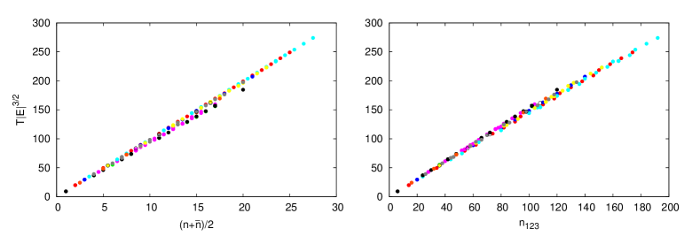
Figure 1: (color on-line) (a) Left panel: The scale-invariant periods $|E|^{3/2}T(w)$ of more than 200 presently known zero-angular-momentum three-body orbits versus one half of the number of all letters in the free-group word $w$ describing the orbit, $N_{w}=n_{w}+{\bar{n}}_{w}$, where $n_{w}$ is the number of small letters ${\tt a}$, or ${\tt b}$, and ${\bar{n}}_{w}$ is the number of capital letters ${\tt A}$, or ${\tt B}$ in the word $w$. (b) Right panel: Same as (a), only in terms of the number of symbols $n_{123}$ in the sequence of symbols (1,2,3) describing the topology of the orbit, see Appendix C. Color code: 1) red = sequence I - butterfly I; 2) green = sequence II - dragonfly; 3) dark blue = sequence III - yin-yang; 4) pink = sequence IVa - moth I; 5) light blue = sequence IVb - butterfly III; 6) yellow = sequence IVc - moth III; 7) black = sequence V - figure-eight; 8) orange = sequence VI - yarn; 9) grey = sequence VII - moth; 10) empty circles = other.

It is clear that the scale-invariant periods $T_{\rm s.i.}$ do not lie on one straight line, but rather on several lines with slightly different slopes, emerging from a small “vertex” area, forming a (thin) wedge-like structure in Fig. 1. All the newly found orbits passing through an Euler configuration, see Supplementary Notes, fit into one of ten sequences, where the fourth (“moth I”) sequence in Ref. Dmitrasinovic:2015 has now been divided into three: a) “moth I $(n,n+1)$”; b) “butterfly III-IV $(n,n+1)$”; c) “moth III $(n,n+1)$”. Moreover, we found two entirely new sequences: 1) “VIIa moth $(n,n)$” and 2) “VIIb moth $(n,n)$”, and one sequence of pure “topological-power satellites” of the moth I orbit.

Each of these ten sequences has an algebraic pattern of free-group elements, see Table 1, associated with it. Here we use the sequence label $(n,m)$ to denote the general form of $(n_{w},{\bar{n}}_{w})$ in that sequence: for example $(n,n)$ means that $n_{w}$ and ${\bar{n}}_{w}$ are equal integers: $n=n_{w}={\bar{n}}_{w}=1,2,3,\ldots$. Then, $n$ can be used to label orbits within the sequence, see Supplementary Notes. By setting $n=0$, or $n=1$, in the second column of Table 1, in each sequence, we can read off the topology of their respective progenitor, which is shown in the third column of Table 1.

Table 1: Typical (non-minimal) free group elements’ $w$ structure for orbits in various sequences, their progenitors, the line parameters $c_{1},c_{2}$, where the $T_{\rm s.i.}(N_{w})$ dependence is fitted as $f(x)=c_{1}x+c_{2}$. Not all words $w(n_{i})$ in any particular sequence need have the presented structure, however, see Supplementary Notes.

	Free group element$w(n)$	progenitor	$c_{1}$	$c_{2}$
I butterfly I $(n,n)$	$({\tt AB})^{2}({\tt abaBAB})^{n}({\tt ab})^{2}({\tt ABAbab})^{n}$	Schubart	$9.957\pm 0.011$	$-0.2\pm 0.2$
II dragonfly $(n,n)$	${\tt bA}({\tt baBA})^{n}{\tt aB}({\tt abAB})^{n}$	isosceles	$9.194\pm 0.004$	$0.04\pm 0.06$
III yin-yang $(n,n)$	$({\tt abaBAB})^{n}{\tt a}({\tt babABA})^{n}{\tt A}$	S-orbit	$9.8667\pm 0.0003$	$0.002\pm 0.004$
IVa moth I $(n,n+1)$	$({\tt abAB})^{n}{\tt A}({\tt baBA})^{n}{\tt B}$	moth I	$9.34\pm 0.06$	$0.7\pm 0.7$
IVb butterfly III $(n,n+1)$	$[({\tt ab})^{2}({\tt AB})^{2}]^{n}{\tt b}[({\tt ba})^{2}({\tt BA})^{2}]^{n}{\tt a}$	butterfly III	$9.967\pm 0.012$	$-0.3\pm 0.3$
IVc moth III $(n,n+1)$	$({\tt babABA})^{n}{\tt A}({\tt abaBAB})^{n}{\tt B}$	Schubart	$9.94\pm 0.04$	$-1.2\pm 0.7$
V figure-eight $(n,n)$	$({\tt abAB})^{n}$	figure-8	$9.2377\pm 0.0014$	$-0.03\pm 0.02$
VI moth I - yarn $(2n,3n)$	$[({\tt abAB}){\tt A}({\tt baBA}){\tt B}]^{n}$	moth I	$9.683\pm 0.002$	$0.01\pm 0.02$
VIIa moth $(n,n)$	$({\tt abAB})^{(n+1)}{\tt a}({\tt baBA})^{n}{\tt b}$	Schubart	$9.61\pm 0.07$	$-0.2\pm 0.7$
VIIb moth $(n,n)$	$({\tt abaBAB})^{(n+1)}{\tt b}({\tt babABA})^{n}{\tt a}$	Schubart	$9.88\pm 0.04$	$-0.7\pm 0.5$

The individual $T_{s.i.}-N_{w}$ graphs are shown in Figs. 2,3, and their free-group patterns are in Table 1. The agreement of separate sequences with the linear functional Ansatz, equation (2), see Fig. 1(b)-(d), is much better than for the aggregate of all orbits, Fig. 1, but the (root-mean-square) variations of line parameters $(c_{1},c_{2})$ reported in Table 1 are generally larger than the estimates numerical errors, thus indicating that equation (2) is still approximate, and not exact, even in these sequences.

Whereas the approximate empirical rule equation (2) now appears established, and its extension to ever-longer periods just a technical difficulty, some deeper questions remain open. For example, the raison d’être of so many periodic orbits remains obscure, let alone the linear relation among their periods.

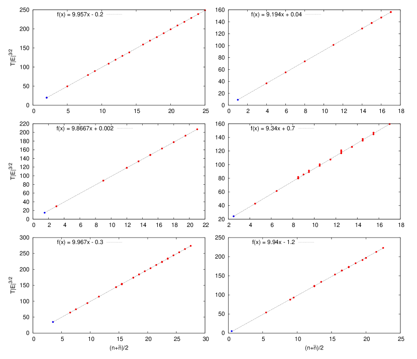
Figure 2: The scale-invariant periods $|E|^{3/2}T(w)$ of zero-angular-momentum three-body orbits versus one half of the number of all letters in the free-group word $w$ describing the orbit, $N_{w}=n_{w}+{\bar{n}}_{w}$, where $n_{w}$ is defined as in Fig. 1. (a) Top left: sequence I - butterfly I, ; (b) Top right: sequence II - dragonfly; (c) Center left: sequence III - yin-yang; (d) Center right: sequence IVa - moth I; (e) Bottom left: sequence IVb - butterfly III; (f) Bottom right: sequence IVc - moth III. The blue points at the lower ends of sequences are the progenitors of the respective sequences, see the text. Progenitors of sequences II, III and IVc, that involve collisions were not used in the fitting procedure, so the validity of the linear Ansatz for these sequences can be evaluated by inspection.

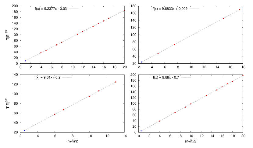
Figure 3: (color on-line) Same as in Fig. 2, except for the following sequences: (a) Top left: sequence V - figure-eight; (b) Top right: sequence VI - yarn; (c) Bottom left: sequence VIIa - moth III $(n,n)$; (d) Bottom right: sequence VIIb - moth III $(n,n)$. The progenitors of sequence VIIa and VIIb were not used in the fitting procedure.

IV Linear stability and progenitor orbits

Perhaps the first hint at a solution to this puzzle was given in Ref. Jankovic:2015 , where it was noticed that the topological satellite orbits in the Broucke-Hadjidemetriou-Hénon (BHH), Broucke1975 ; Broucke1975b ; Hadjidemetriou1975a ; Hadjidemetriou1975b ; Hadjidemetriou1975c ; Henon1976 ; Henon1977 , family of orbits with non-zero angular momentum, exist only when their progenitor is linearly stable. There is a theorem, due to Birkhoff and Lewis Birkhoff_Lewis:1933 , see also §3.3 (by Jürgen Moser) in Ref. Klingenberg:1978 , which holds for systems with three d.o.f. and implies the existence of infinitely many periodic orbits . So, whereas the Birkhoff-Lewis theorem might solve one part of the puzzle, it does not say anything about the relation of topologies and periods. There is, however, another (the so-called “twist”) condition underlying this theorem, which we shall not try to check here - we simply conjecture that the Birkhoff-Lewis theorem holds for the linearly stable periodic three-body orbits. Linear stability of periodic orbits is tested numerically, see below, and thus the conjecture of Birkhoff-Lewis theorem can be falsifed.

We have analyzed linear stability of all zero-angular-momentum three-body orbits and tabulated the linearly stable ones in Table 2. The Floquet exponents $\nu_{j}$, and the linear stability coefficients $\lambda_{j}=\exp(\pm 2\pi i\nu_{j})$, are the standard ones, as defined in Ref. Dmitrasinovic:2016 .

Table 2: The Floquet exponents $\nu_{j}$, where $\lambda_{j}=\exp(\pm 2\pi i\nu_{j})$ define the linear stability coefficients of linearly stable periodic three-body orbits.

	$\nu_{1}$	$\nu_{2}$
S-orbit	0.131093	0.470591
Moore 8	0.298093	0.00842275
NC1 ($8^{7}$)	0.27216	0.158544
V.17.H (O13 = $8^{17}$)	0.31573	0.0002988
V.17.I (O14 = $8^{17}$)	0.0435411	0.00262681
V.17.J (O15 = $8^{17}$)	0.0435411	0.00262681
II.11.A (bumblebee)	0.137149	0.0325135
IVa.2.A (moth I)	0.159013	0.491881
IVa.4.A (moth II)	0.108451	0.0886311
IVb.3.A (butterfly III)	0.378728	0.00173642
I.5.A	0.170764	0.001476
I.14.A	0.443006	0.000121435
II.17.B	0.138698	0.0335924
III.13.A.$\beta$	0.175816	0.000655417
IVb.9.A	0.194186	0.000561819
IVc.12.B	0.0863933	0.00394124
IVc.17.A	0.0442047	0.00206416
VIIa.11.A	0.416228	0.0088735
VIIb.7.A	0.27753	0.0360425
VIIb.9.A	0.216455	0.0584561
VIIb.13.A	0.0621421	0.0141894

We note that two orbits, “butterfly III” and “moth I”, lie at the origins of two “linear sequences” of “non-topological-power satellite” orbits observed among the original 13 orbits Dmitrasinovic:2015 .

Thus, the manifest candidates for progenitors are: 1) “figure-eight” for the sequence V “figure-eight $(n,n)$”; 2) “butterfly III” for the sequence IVb “butterfly III $(n,n+1)$”; and 3) “moth I” for the sequences IVa “moth I $(n,n+1)$” and VI “moth I - yarn $(2n,3n)$”. These three progenitors are collisionless orbits with three degrees-of-freedom, that are linearly stable.

Next we extend this reasoning to sequences of periodic three-body orbits with collisional progenitors.

1) The parent orbit of sequence II “dragonfly $(n,n)$” is Broucke’s isosceles triangle orbit Broucke1979 ; Zare1998 , that involves two-body collisions. This orbit always stays in an isosceles triangle configuration, thus eliminating one degree-of-freedom, and is linearly stable Broucke1979 ; Zare1998 , so it also satisfies the Poincaré-Birkhoff theorem.

2) The parent orbit of the “yin-yang” sequence is the collisional “S-orbit” of Refs. Martynova2009 ; Iasko2014 .

3) The Schubart orbit Schubart1956 is the progenitor of four sequences: I, IVc, VIIa and VIIb, see Table 1 and Supplementary Notes. The Schubart orbit is linearly stable in three spatial dimensions, Henon1976 ; Henon1977 , but due to its collinear nature, it has only two degrees-of-freedom. As it has two degrees-of-freedom, it satisfies the Poincaré-Birkhoff theorem Birkhoff:1935 ; Siegel_Moser:1971 ; Moser_Zehnder:1979 , which also predicts the existence of infinitely many orbits .

Thus, we have shown a definite correlation between the sequences in Table 1 and linear stability of the progenitor orbit in each sequence.

V Virial theorem and analyticity of the action

The remaining mysteries are: (i) why are the $T_{s.i.}(N_{w})$ graphs linear, and (ii) why are the slopes of different sequences so close to each other?

Our answers to these questions are still not proven in a sufficiently rigorous way. Therefore, we shall present them here in the same, or similar way, as they were discovered; otherwise the motivation, and the weak points of our arguments might be lost.

It should be clear that the mere formulation of $T_{s.i.}=T|E|^{3/2}$ depends crucially on the homogeneity of the Newtonian potential: the exponent $3/2$ follows from the Newtonian potential’s degree of homogeneity $\alpha=1$, see Suvakov:2014 ; Dmitrasinovic:2015 . So, one may ask if the same, or similar behaviour occurs in other homogeneous potentials? A (partial) answer to this question was provided in Ref. Dmitrasinovic:2017 , where periodic three-body orbits in the so-called strong potential $V^{\alpha=2}(r)\simeq-1/r^{2}$ and their relation to topology were studied, which has led to our proposed answer to question (i). The strong potential $V^{\alpha=2}(r)\simeq-1/r^{2}$, is also homogeneous, see Appendix D.

It was shown in Ref. Dmitrasinovic:2017 that the periodic solutions to the three-body problem in the strong potential form sequences, very much like those in the Newtonian potential shown in Sect. III, but their periods do not increase linearly with the topological complexity $N_{w}$ of the orbit. Rather, it is the action integral, $S_{min}\simeq N_{w}$, that rises linearly with $N_{w}$, which fact can be understood using Cauchy’s residue theorem, which is based on the analyticity of the action integral,

$$S^{\alpha=2}_{min}=-{2}\int_{0}^{T}V^{\alpha=2}({\bf r}(t))dt,$$

where ${\bf r}(t)$ is a periodic solution to the equations-of-motion (e.o.m.) at fixed energy $E=0$, see Appendix E.

But, in the Newtonian potential the action of (any) periodic orbit is proportional to its period $S^{\alpha=1}_{min}(T)=3|E|T$, see equation (9), derived in Appendix D.2. So, the scale-invariant period $T_{s.i.}$ must depend in the same way on the topological complexity $N_{w}$ of the orbit as the corresponding action $S^{\alpha=1}_{min}(T)$. The question now arises if the same argument as in Dmitrasinovic:2017 , about the analyticity of the action $S^{\alpha=1}_{min}(T)$ can be extended to the Newtonian potential?

In the Newtonian potential this argument becomes more complicated because the hyper-radius $R=|Z|$ is not constant in Newtonian three-body orbits, and the problem becomes one in the calculus of two complex variables, see Appendices A and E. This leads to new possibilities that have not been considered thus far. Indeed, the second complex variable in the Newtonian potential immediately leads to the possibility that there is a pole in the second complex variable $Z$, which could lead to non-zero contributions to the integral, and thus change the $T_{s.i.}(N_{w})$ functional dependence, under right conditions.

Assuming that the variation of periodic orbits in the second complex variable $Z$ is limited such that no new poles arise in the action integral, see Appendix E, we may conclude that

$$S^{\alpha}_{min}=\left(\frac{\alpha+2}{\alpha-2}\right)E\leavevmode\nobreak\ T\simeq N_{w}.$$

This cannot be true in general, however: A moment’s thought shows that the linear dependence cannot hold in the harmonic oscillator, as all harmonic oscillatory motions have the same period there. More formally, equation $S^{\alpha}_{min}=\left(\frac{\alpha+2}{\alpha-2}\right)E\leavevmode\nobreak\ T$, implies that the action of a periodic orbit in the harmonic oscillator always vanishes $S_{min}^{\alpha=-2}=0$. Moreover, we note that the action integral equation (8) must have (at least one) pole if the residue theorem should hold. Consequently, there is an upper bound on the exponent: $\alpha\geq 0$, for which this kind of action-topology dependence can exist.

These arguments provide also a (possible) answer to question (ii) above, as the slope of of the $T_{s.i.}(N_{w})$ graph depends on the residue(s) at the same poles in all sequences, the main difference being the ordering of circles around the poles, i.e., of the Riemann sheet(s) one is on (“crossings of branch cuts”), see Appendix E.

Of course, the foregoing arguments do not constitute a mathematical proof - the missing dots on the i’s and crosses on the t’s, or, perhaps more interestingly, counter-arguments/proofs - ought to be supplied by the interested reader.

VI Summary, Discussion and Outlook

We have shown that:

1) The presently known periodic three-body orbits with vanishing angular momentum and passing through an Euler configuration, can be classified into 10 sequences according to their topologies. Each sequence probably extends to infinitely long periods, and emerges from one of six linearly stable (shortest-period) progenitor orbits.

2) Numerically, the scale-invariant periods of orbits in each sequence obey linear dependences on the number of symbols in the algebraic description of the orbit’s topology.

3) There is a possible explanation for the existence of this infinity of periodic orbits, in the form of Birkhoff-Lewis theorem, provided that each progenitor orbit also satisfies the “twist” condition Birkhoff_Lewis:1933 .

4) Some of the longer-period orbits are linearly stable: a) the seventh satellite of “figure-8” orbit, ; b) moth II, which lies in, but is not the progenitor of the “moth I” sequence; and c) the “bumblebee” orbit, which lies in, but is not the progenitor of the “dragonfly” sequence.

We note that in 1976 Henon1976 , Hénon established the linear stability of many orbits with non-vanishing angular momenta ($L\neq 0$) in the Broucke-Hadjidemetriou-Hénon family. The topological-power satellites of these linearly stable BHH orbits were discovered only recently Jankovic:2015 , where an $L\neq 0$ version of the period-topology linear dependence equation (2) was checked numerically, as well. The agreement there is also (only) approximate, as a small, but numerically significant discrepancy exists.

Furthermore, Ref. Dmitrasinovic:2017 indicates that a linear dependence of the action, but not of the period, on the topology exists also in the case of periodic three-body orbits in the so-called strong Jacobi-Poincaré potential, which is in agreement with the virial theorem, see Appendix D. The argument in Ref. Dmitrasinovic:2017 can be extended to the Newtonian potential, but it becomes a complicated question in the calculus of two complex variables .

Our results are generic, so they imply that similar linear relations may be expected to hold for 3-body orbits in the Coulombian , and in all other homogeneous potentials containing poles.

Moreover, similar functional dependences might also hold for 4-, 5-, 6-body etc. orbits in the Newtonian potential.

Our results also raise new questions:

1) Each of the six progenitors generates a family of orbits, at different masses and non-vanishing angular momenta, e.g. the Schubart colliding orbit Schubart1956 , generates the BHH family of collisionless orbits with non-zero angular momenta, that describe the majority of presently known triple-star systems. The remaining five progenitors may now be viewed as credible candidates for astronomically observable three-body orbits, provided that their stability persists under changes of mass ratios and of the angular momentum. Those dependences need to be explored in detail.

2) Checking the “twist” condition of the Birkhoff-Lewis theorem, for each progenitor orbit, is a task for mathematicians, as is the explanation of the topologies of the so-predicted orbits: why do these sequences exist and not some others?

3) The question of existence of other stable two-dimensional colliding orbits, and of new sequences of periodic orbits that they (may) generate. Rose’s new linearly stable colliding orbits DanyaRose are particularly interesting in this regard. Turning the foregoing argument around, one can use any newly observed sequence of orbits to argue for the the existence of its, perhaps as yet unknown, progenitor.

4) A remaining mystery is why are the slopes of different sequences so close to each other?

Appendix A Three-Body Variables

The graphical representation of the three-body system can be simplified with the use of translational and rotational invariance – by changing the coordinates to the Jacobi ones Jacobi:1843 . Jacobi or relative coordinates are defined by two relative coordinate vectors, see Fig. 4:

$${\bm{\rho}}=\frac{1}{\sqrt{2}}({\bf r}_{1}-{\bf r}_{2}),\leavevmode\nobreak\ \leavevmode\nobreak\ \leavevmode\nobreak\ \leavevmode\nobreak\ {\bm{\lambda}}=\frac{1}{\sqrt{6}}({\bf r}_{1}+{\bf r}_{2}-2{\bf r}_{3}).$$ (3)

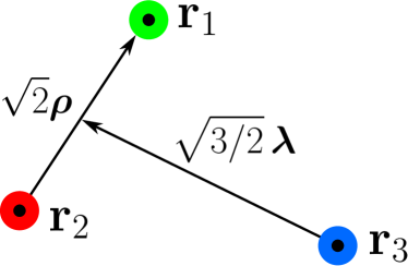
Figure 4: The two three-body Jacobi coordinates ${\mbox{\boldmath$\rho$}},{\mbox{\boldmath$\lambda$}}$.

Three independent scalar variables can be constructed from Jacobi coordinates: $\bm{\rho}^{2}$, $\bm{\lambda}^{2}$ and $\bm{\rho}\cdot\bm{\lambda}$. The overall size of the orbit is characterized by the hyperradius $R=\sqrt{\bm{\rho}^{2}+\bm{\lambda}^{2}}$. These scalar variables are connected to the unit vector with Cartesian components Montgomery:1998 :

$$\hat{\mathbf{n}}=\left(\frac{2\bm{\rho}\cdot\bm{\lambda}}{R^{2}},\frac{\bm{\lambda}^{2}-\bm{\rho}^{2}}{R^{2}},\frac{2(\bm{\rho}\times\bm{\lambda})\cdot\mathbf{e}_{z}}{R^{2}}\right).$$ (4)

Therefore, every configuration of three bodies (shape of the triangle formed by them, independent of size) can be represented by a point on a unit sphere. This sphere is called the shape-sphere.

Every relatively periodic orbit of a three-body system is therefore represented on the shape-sphere by a closed curve (collisionless solutions), a finite open section of a curve (free-fall and colliding solutions), or a point (Lagrange–Euler solutions). One example, the figure-eight orbit, is illustrated in Fig. 5.

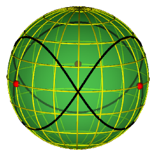
Figure 5: The shape-space sphere: the figure-eight orbit (solid black curve); three two-body collision points (red), singularities of the potential, lie on the equator.

The north and the south pole of the shape-sphere correspond to equilateral triangles, while the equator corresponds to degenerate triangles, where the bodies are in collinear configurations (syzygies). There are three points on the equator that correspond to two-body collision points – the singularities of the potential, see Fig. 5.

Two orbits with identical representations on the shape-sphere are considered to be the same solution. For example, periodic orbits subjected to symmetry transformations, such as translations, rotations, dilations, reflections of space and time, all have identical curves on the shape-sphere and are counted as one.

Size or energy scaling, ${\bf r}\rightarrow\alpha{\bf r}$, and the equations of motion imply $t\rightarrow\alpha^{3/2}t$ Landau . Therefore, the velocity scales as ${\bf v}\rightarrow{\bf v}/\sqrt{\alpha}$, the total energy scales as $E\rightarrow\alpha^{-1}E$, and the period $T$ as $T\rightarrow\alpha^{3/2}T$. Consequently, the combination $|E|^{3/2}T$ is invariant under scale transformations and we call it scale invariant period $T_{s.i.}=|E|^{3/2}T$. It is always possible to remove one of the three scalar variables by changing the hyper-radius to the desired value by means of these scaling rules.

Appendix B Montgomery’s topological identification method

A curve corresponding to a collisionless periodic orbit can not pass through any one of the three two-body collision points. Stretching this curve across a collision point would therefore change its topology. The classification problem of closed curves on a sphere with three punctures is given by the conjugacy classes of the fundamental group, which is in this case the free group on two letters (${\tt a,b}$), see Fig. 6.

This abstract notation has a simple geometric interpretation: it classifies closed curves in a plane with two punctures according to their topologies. The shape sphere can be mapped onto a plane by a stereographic projection using one of the punctures as the north pole, see Fig. 7. The selected puncture is thusly removed to infinity, which leaves two punctures in the (finite) plane. Any closed curve on the shape sphere (corresponding to a periodic orbit) can now be classified according to the topology of its projection in the plane with two punctures.

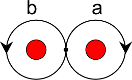
Figure 6: The two elements $({\tt a,b})$ of the free group.

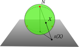
Figure 7: Stereographic projection of a sphere onto a plane. Three two-body collision points (solid red) lie on a meridian (dashed circle), with one of them being at the north pole (denoted by the letter $N$).

Topology of a curve can be algebraically described by a “word” - a sequence of letters ${\tt a}$, ${\tt b}$, ${\tt A}$ and ${\tt B}$ - which is, more formally, an element of the free group $F_{2}$. Here ${\tt a}$ denotes a clockwise full turn around the right-hand-side puncture, ${\tt b}$ the counter-clockwise full turn around the left-hand-side puncture (see Fig. 6), and the upper case letters denote their inverse elements ${\tt a}^{-1}={\tt A}$ and ${\tt b}^{-1}={\tt B}$.

A specific periodic orbit can be equally well described by several different sequences of letters. As there is no preferred starting point of a closed curve, any other word that can be obtained by a cyclic permutation of the letters in the original word represents the same curve.

The conjugacy class of a free group element (word) contains all cyclical permutations of the letters in the original word. For example, the conjugacy class of the free group element ${\tt aB}$ also contains the cyclically permuted word ${\tt Ba}$. The class of topologically equivalent periodic orbits therefore corresponds not merely to one specific free group element, but to the whole conjugacy class.

Time-reversed orbits are represented by the inverse elements of the original free group elements. Naturally, they correspond to physically identical solutions, but they generally form different words (free group elements) with different conjugacy classes.

Another ambiguity is related to the choice of the puncture to be used as the north pole of the stereographic projection (of the sphere onto the plane). A single loop around any one of the three punctures on the original shape sphere (denoted by ${\tt a}$ or ${\tt b}$) must be equivalent to the loop around either of the two remaining punctures. But as can be seen in Fig. 7, a simple loop around the third (“infinite”) puncture on the shape sphere corresponds to ${\tt aB}$, a loop around both poles in the plane. Therefore, ${\tt aB}$ must be equivalent to ${\tt a}$ and ${\tt b}$.

Some periodic solutions have free group elements that can be written as $w^{k}=w^{k}({\tt a,b,A,B})$, where $w=w({\tt a,b,A,B})$ is a word that describes some solution, and $k$ is an integer. Such orbits will be called topological-power satellites. For example, the orbits with free group element $({\tt abAB})^{k}$ are called figure-eight ($k$) satellites, and are all free from the stereographic projection ambiguity.

Appendix C Tanikawa and Mikkola’s (syzygy) method of topological identification

There is an alternative method of assigning a sequence of three symbols, in this case three digits $({\tt 1,2,3})$, to any given “word” in the free group $F_{2}$. It has been proposed for collisionless orbits, by Ref. Tanikawa:2008 , see also Ref. Moeckel:2014 , to use the sequence of syzygies (collinear configurations) as a symbolic dynamics for the 3-body problem.

The rules for converting “words” consisting of letters ${\tt a}$ , ${\tt b}$, ${\tt A}$, ${\tt B}$ into “numbers” consisting of three digits - $({\tt 1,2,3})$ - are as follows: (i) make the substitution ${\tt a=12}$, ${\tt A=21}$, ${\tt b=32}$, ${\tt B=23}$; (ii) ${\tt 11=22=33}$ = empty sequence (“cancellation in pairs rule”). So, for example:

(1) the symbolic sequence corresponding to the BHH family of orbits, ${\tt aB=1223=13}$ is equivalent, by way of cyclic permutations, to: ${\tt a=12}$ and to ${\tt B=23}$, as one would expect intuitively. Thus we see that the “lengths” $N_{n}$, i.e., the number of symbols in a sequence are identical for all three symbolic sequences representing the BHH family, $N_{n}({\tt 13})$=$N_{n}({\tt 12})$=$N_{n}({\tt 23})$, unlike the Montgomery’s method, where $N_{w}({\tt aB})\neq N_{w}({\tt a})=N_{w}({\tt B})$. This indicates that the “lengths” $N_{n}(w)$ are good algebraic descriptors of the complexity of an orbit’s topology.

(2) the symbolic sequence ${\tt abAB=(12)(32)(21)(23)=12322123=123123=(123)^{2}}$ corresponding to the figure-eight orbit is now manifestly invariant under cyclic permutations, ${\tt 1}\to{\tt 2}\to{\tt 3}$ and ${\tt 1}\to{\tt 3}\to{\tt 2}$, whereas it is so only in a non-manifest way in the two-letter scheme. Here, also, the “length” $N_{n}(w)$ is also a good algebraic descriptor of the complexity of an orbit’s topology.

Note that:

1. As stated above, the numbers ${\tt 1}$, ${\tt 2}$, and ${\tt 3}$ can be viewed as denoting syzygies, i.e., crossings of the equator on the shape sphere, in one of three corresponding segments on the said equator, where the index of the body passing between the other two is used as a symbol.

2. Each symbol is its own inverse, which accounts for the “cancellation in pairs” rule . This circumstance leads to the reduction (by a factor of two) of the number of symbolic sequences denoting one topology, as the time-reversed orbit has an identical symbolic sequence to the original one (which is not the case in the two-letter scheme); and

3. That the cyclic permutation symmetry indicates irrelevance of which syzygy is denoted by which digit.

In this way, we have restored the three-body permutation symmetry of the problem into the algebraic notation describing the topology of a periodic three-body orbit, albeit at the price of having three symbols, rather than two. This restoration of permutation symmetry also implies an absence of the “automorphism ambiguity” Dmitrasinovic:2015 . Such three-symbol sequences have been used e.g. in Refs. Tanikawa:2008 ; Moeckel:2014 to identify the topology of periodic three-body orbits.

The length of a sequence of symbols necessary to describe any given topology generally increases by a factor close to 1.5 as one switches from two letters $N_{w}$ to three digits $N_{s}$, as symbols used, i.e., $N_{s}\simeq 1.5N_{w}$. The precise value of this proportionality factor ($\simeq 1.5$) is not important for our purposes, as we shall be concerned with the length(s) of symbolic sequences with a well-defined algebraic form, such as $w_{1}(w_{2})^{n}w_{3}(w_{4})^{n}$, where $n=1,2,3,\cdots$. In such a case, the following relation holds $N[w_{1}(w_{2})^{n}w_{3}(w_{4})^{n}]\simeq N[w_{1}w_{3}]+nN[w_{2}w_{4}]$ using either set of symbols for $w_{i}$. Only the value of the slope parameter changes as one switches from one set to another. Of course, it is an additional mystery if and when the slopes of different sequences happen to coincide.

Appendix D Virial theorem and the action of periodic orbits in homogeneous potentials

D.1 The Lagrange-Jacobi identity and the virial theorem

We know that the Lagrange-Jacobi identity Jacobi:1843 ,

$$\frac{1}{2}\frac{dG}{dt} = 2K_{total}+\alpha V^{\alpha}_{total},\$$ (5)

where $G=\sum_{i=1}^{N}{\bf q}_{i}\cdot{\bf p}_{i}$ is the so-called virial, gives a relation between kinetic $K_{total}=\sum_{i}K_{i}$ and potential energy $V_{total}^{\alpha}$, for homogeneous potentials with homogeneity degree $-\alpha$. One example of such a homogeneous potential is the sum of two-body terms $\sum_{i<j}V_{\alpha}(r_{ik})$, where $V_{\alpha}(r_{ik})\simeq-1/r_{ik}^{\alpha}$ is a power-law interaction . Here $r_{ik}$ is the distance between two particles, and $\alpha$ is a positive real number.

For periodic motions, with period $T$, this identity can be integrated to yield

$$\frac{1}{2}\int_{0}^{T}dt\frac{dG}{dt} = \frac{1}{2}\left(G(T)-G(0)\right)=0$$ (6)

$$= \int_{0}^{T}(2K_{total}+\alpha V_{total}^{\alpha})dt\$$

which tells us that the time integral of the kinetic energy is related to the time integral of the potential energy:

$$\int_{0}^{T}dtK_{total}=-\frac{\alpha}{2}\int_{0}^{T}dtV_{total}^{\alpha}$$

Energy conservation

$$E=K_{total}+V_{total}^{\alpha}$$

implies

$$E=\frac{1}{T}\int_{0}^{T}(K_{total}+V_{total}^{\alpha})dt=\frac{1}{T}\int_{0}^{T}(-\frac{\alpha}{2}V_{total}^{\alpha}+V_{total}^{\alpha})dt$$

which leads to the equipartition of energy (or “virial”) theorem:

$$E = \left(\frac{\alpha-2}{-2}\right)\frac{1}{T}\int_{0}^{T}V^{\alpha}(r(t))dt\equiv\left(\frac{\alpha-2}{-2}\right)\langle V^{\alpha}(r)\rangle$$ (7)

$$E = \left(\frac{\alpha-2}{\alpha}\right)\frac{1}{T}\int_{0}^{T}K({\dot{r}}(t))dt\equiv\left(\frac{\alpha-2}{\alpha}\right)\langle K({\dot{r}}(t))\rangle\$$ (8)

which holds exactly for periodic orbits. This, in turn, reduces the action $S$ to one or another time integral.

D.2 The action for three-body orbits in a homogeneous potential

The (minimized) action of a periodic n-body orbit in a homogeneous potential $V^{\alpha}(r)\simeq-1/r^{\alpha}$ is

$$S_{min}=\int_{0}^{T}L(q(t),{\dot{q}}(t))dt=\int_{0}^{T}\left(T({\dot{r}}(t))-V^{\alpha}(r(t))\right)dt,$$

leads to

$$S^{\alpha}_{min}(T)=\left(\frac{\alpha+2}{\alpha-2}\right)E\leavevmode\nobreak\ T,$$ (9)

which depends only on the energy $E$ and period $T$ of the orbit. Note the singularity on the right-hand-side of equation (9) at $\alpha=2$, which demands that $E=0$ in that case. For the Newtonian case, $\alpha=1$, equation (9) leads to

$$S^{\alpha=1}_{min}(T)=-3ET=3|E|T,$$

as claimed in Dmitrasinovic:2015 .

Appendix E Complex variables and analytic properties of the action

Here we follow closely Appendix C in Ref. Dmitrasinovic:2017 . The minimized action $S^{\alpha}_{min}=\int_{0}^{T}L(q(t),{\dot{q}}(t))dt$ of a periodic orbit $q(t)$ in the homogeneous (power) potential $V^{\alpha}(r)$, written as a time integral of twice the kinetic energy $K$ over period $T$,

$$S^{\alpha}_{min}(T) = \left(\frac{\alpha+2}{\alpha}\right)\sum_{i=1}^{3}\int_{0}^{T}\frac{{\bf p}_{i}^{2}}{2m}dt=\left(\frac{\alpha+2}{\alpha}\right)\sum_{i=1}^{3}\int_{{\bf r}_{i}(0)}^{{\bf r}_{i}(T)}{\bf p}_{i}\cdot d{\bf r}_{i}$$ (10)

where $m=1$, can be expressed as a closed-contour integral of two complex variables. After shifting to the relative-motion variables, $({\bm{\rho}},{\bm{\lambda}})$, one finds

$$S^{\alpha}_{min}(T)=\left(\frac{\alpha+2}{\alpha}\right)\left(\int_{{\bm{\rho}}(0)}^{{\bm{\rho}}(T)}{\bf p}_{\rho}\cdot d{\bm{\rho}}+\int_{{\bm{\lambda}}(0)}^{{\bm{\lambda}}(T)}{\bf p}_{\lambda}\cdot d{\bm{\lambda}}\right)$$

The real Jacobi two-vectors ${\bm{\rho}}$ and ${\bm{\lambda}}$ may be replaced with two complex variables

$$z_{\rho}=\rho_{x}+i\rho_{y},\leavevmode\nobreak\ z_{\lambda}=\lambda_{x}+i\lambda_{y},$$

so that the action $S^{\alpha}_{min}$, can be rewritten as a (double) closed contour integral in two complex variables:

$$S^{\alpha}_{min}(T)=\left(\frac{\alpha+2}{\alpha}\right)\left(\int_{z_{\rho(0)}}^{z_{\rho(T)}}{\dot{z}}_{\rho}^{*}dz_{\rho}+\int_{z_{\lambda}(0)}^{z_{\lambda}(T)}{\dot{z}}_{\lambda}^{*}dz_{\lambda}\right).$$

Note that the periodicity of motion ${\bm{\rho}}(0)={\bm{\rho}}(T)$, ${\bm{\lambda}}(0)={\bm{\lambda}}(T)$ implies $z_{\rho}(T)=z_{\rho}(0)$ and $z_{\lambda}(T)=z_{\lambda}(0)$, which makes this integral a closed contour one

$$S^{\alpha}_{min}=\left(\frac{\alpha+2}{\alpha}\right)\left(\oint_{C_{\rho}}{\dot{z}}_{\rho}^{*}dz_{\rho}+\oint_{C_{\lambda}}{\dot{z}}_{\lambda}^{*}dz_{\lambda}\right).$$

If there were only one complex variable, then the so-defined function would be analytic. Indeed, the action of two-body elliptic motion in the Newtonian potential has been evaluated using Cauchy’s residue theorem in Sect. 18.16 of Ref. Pars:1964 , and in Sect. 11.8 in Ref. Marmi:2006 . With two complex variables, there is no such guarantee, however. Moreover, the residue theorem for functions of two complex variables is a more complicated matter, see Refs. Fuks ; Hormander ; Shabat ; Freitag .

The existence and positions of poles in this (double) contour integral are not manifest in its present form; the same integral is given by equation (7) in Appendix D.2, $S^{\alpha}_{min}(T)=\left(\frac{\alpha+2}{-2}\right)\int_{0}^{T}V^{\alpha}(r(t))dt$, due to the virial theorem, however, where the potential $V^{\alpha}({r}(t))$ is known to have three singularities (simple poles) at three binary collisions and the time-evolution dependence $r(t)$ of the periodic orbit, which parametrizes the contour. For the Newtonian potential $\alpha=1$ the binary collisions are regularizable, and this integral has been studied by K. F. Sundman Sundman:1907 with the result that the functions $r_{k}(u),1\leq k\leq 3$, are holomorphic in a strip $|\mathrm{Im}\leavevmode\nobreak\ u|<\delta$ of the complex plane $u\in C$ which contains the real axis, see §2.3. in Ref. Arnold:2006 . Since $S^{\alpha=1}_{min}(T)=S(T)=-\left(\frac{3}{2}\right)u(T)$, we know that the trajectories $r_{k}(S),1\leq k\leq 3$ are holomorphic functions of the action $S$ in a strip $|\mathrm{Im}\leavevmode\nobreak\ S|<\delta$ of the complex plane $S\in C$ which contains the real axis.

Note the following implications of this result: 1) for non-singular potentials ($\alpha<0$) there are no poles in the potential, and consequently no poles encircled by the contour, so the residue vanishes; 2) for singular potentials ($2>\alpha>0$) there are poles in the potential, but the residue depends on the integration contour, i.e., on the trajectory on the shape sphere and its topology $w$; 3) if the integration contour, i.e., the trajectory on the shape sphere repeats $k$ times the topologically equivalent path, then, for singular potentials ($2>\alpha>0$), the residue equals $k$ times the single path residue.

Next, we switch from the real $({\bm{\rho}},{\bm{\lambda}})$, or complex $(z_{\rho},z_{\lambda})$ Cartesian Jacobi variables to the curvilinear hyper-spherical variables: the real hyper-radius $R$ and the overall rotation angle $\Phi=\frac{1}{2}(\varphi_{\rho}+\varphi_{\lambda})$, and the two angles parametrizing the shape-sphere, e.g. $(\theta=(\varphi_{\rho}-\varphi_{\lambda}),\chi=2{Tan}^{-1}(\frac{\rho}{\lambda}))$. Here $(\varphi_{\rho},\varphi_{\lambda})$ are the angles subtended by the vectors $({\bm{\rho}},{\bm{\lambda}})$ and the $x$-axis. Equivalently, we may use the complex variables $Z$, defined by $(R,\Phi)$ and $z$, defined by way of a stereographic projection from the shape-sphere parametrized by $(\theta,\chi)$.

The variable $Z$ has limited (bounded) variation for all periodic orbits (with zero angular momentum) studied in this paper. Indeed, the value of $R=|Z|=0$ occurs only in the “triple collision” (“der Dreierstoss”) orbits, which does not happen in our case. The condition $\Phi$ = const. is trickier, however, because there are “relatively periodic” solutions with vanishing angular momentum ($L=0$) and a non-zero change $\Delta\Phi\neq 0$ of angle $\Phi$ over one period. All of the orbits considered in this paper are absolutely periodic, i.e., they have $\Delta\Phi$ = 0 over one period, so this caveat does not apply. Therefore one may eliminate the complex variable $Z$ from further consideration, at least for the orbits considered here, and the problem becomes (much) simpler.

Thus, we see that the complex integration contour $C_{z}$ relevant to Cauchy’s theorem, $S_{min}=2i\pi\sum{Res}$, for the considered periodic orbits, is determined solely by the orbit’s trajectory on the shape sphere: the only poles relevant to this contour integral are the two-body collision points on the shape sphere. Consequently, the periodic orbits’ minimized action (integral) is determined (predominantly) by the topology of the closed contour on the shape sphere, i.e., by the homotopy group element of the periodic orbit, unless there is a closed contour in the $Z=(R,\Phi)$ variable, as well.

Repeated $k$-fold loops of the contour lead to $k$ times the initial integral, i.e., $S_{min}(w^{k})=2ki\pi\sum{Res}=kS_{min}(w)$, or, equivalently $T_{s.i.}(w^{k})=kT_{s.i.}(w)$, as observed in topological satellite orbits in Sect. III. Crossings of branch cuts provide for the change of residue(s) of the pole(s) at different values of $k$, which may account for the different values of ${Res}$, i.e., for different slopes of $T_{s.i.}(N_{w})$ graphs in different sequences.

Detailed study of analytic properties of the action should be a subject of interest to pure mathematicians, however, Feynman:1964 .

References

- (1) E. H. Bruns, Acta Math. 11, 25 (1887) (in German).
- (2) C. Moore, Phys. Rev. Lett. 70, 3675–3679 (1993).
- (3) A. Chenciner and R. Montgomery, Ann. Math. 152, 881–901 (2000).
- (4) A. I. Martynova, V. V. Orlov, and A. V. Rubinov, Astron. Rep. 53, 710 (2009).
- (5) M. Šuvakov, and V. Dmitrašinović, Phys. Rev. Lett. 110, 114301 (2013).
- (6) R. Vernić, Hrvatsko Prirod. Društvo Clas. Mat. Fiz. Astron., Ser. 2, 8, 247-266 (1953).
- (7) R. F. Arenstorf, pp. 55–68 in “Differential Equations and Dynamical Problems”, edited by J. K. Hale and J. P. LaSalle, Academic Press (1967).
- (8) R. Broucke and D. Boggs, Celest. Mech. 11, 13 (1975).
- (9) V. Dmitrašinović, A. Hudomal, M. Shibayama and A. Sugita, “Newtonian Periodic Three-Body Orbits with Zero Angular Momentum: Linear Stability and Topological Dependence of the Period”, arXiv:1705.03728v2 [physics.class-ph] (2017).
- (10) M. Šuvakov, Celest. Mech. Dyn. Astron. 119, 369-377 (2014).
- (11) P. P. Iasko and V. V. Orlov, Astron. Rep. 58, 869-879 (2014).
- (12) M. Šuvakov and M. Shibayama, Celest. Mech. Dyn. Astron. 124, 155-162 (2016).
- (13) D. Rose, “Geometric phase and periodic orbits of the equal-mass, planar three-body problem with vanishing angular momentum”, Ph.D. thesis, University of Sydney (2016). Available at https://ses.library.usyd.edu.au/handle/2123/14416
- (14) X. Li and S. Liao, Sci. China-Phys. Mech. Astro. Vol. 60 No. 12: 129511 (2017). (doi: 10.1007/s11433-017-9078-5). Initial conditions can be found at the website: http://numericaltank.sjtu.edu.cn/three-body/three-body.htm
- (15) V. Dmitrašinović and M. Šuvakov, Phys. Lett. A 379, 1939-1945 (2015).
- (16) G. D. Birkhoff and D. C. Lewis, Ann. di Mat. (4) 12, 117-133 (1933).
- (17) R. Montgomery, Nonlinearity 11, 363 - 376 (1998).
- (18) K. Tanikawa and S. Mikkola, “A trial symbolic dynamics of the planar three-body problem”, arXiv:0802.2465, (2008).
- (19) M. Šuvakov, and V. Dmitrašinović, Am. J. Phys. 82, 609-619 (2014).
- (20) http://three-body.ipb.ac.rs/sequences.php
- (21) R. Moeckel and R. Montgomery, Nonlinearity 28, 1919 (2015).
- (22) G. D. Birkhoff, Mem. Pon. Acad. Sci. Novi Lyncaei (3) 1, 85-216 (1935).
- (23) C. L. Siegel and J. K. Moser, “Lectures on Celestial Mechanics”, Springer-Verlag Berlin Heidelberg (1971).
- (24) J. K. Moser and E. J. Zehnder, “Notes on Dynamical Systems”, American Mathematical Society, Providence R. I. (2000).
- (25) W. Klingenberg, “Lectures on Closed Geodesics”, Springer-Verlag Berlin Heidelberg New York (1978).
- (26) L. A. Pars, “Analytical Dynamics” (London, UK: Heinemann, 1965).
- (27) A. Fasano and S. Marmi, “Analytical Mechanics: An Introduction”, Oxford University Press, Oxford, UK (2006).
- (28) K. F. Sundman Acta Soc. Sci. Fennicae 34, no. 6, 144-151 (1907); K. F. Sundman, Acta Math. 36, 105-179 (1912) (in French).
- (29) V. I. Arnold, V. V. Kozlov, A. I. Neishtadt, “Mathematical Aspects of Classical and Celestial Mechanics”, 3rd edition, Encyclopaedia of Mathematical Sciences Volume 3 Dynamical Systems III, Springer-Verlag Berlin Heidelberg (2006).
- (30) C. G. J. Jacobi, “Vorlesungen über Dynamik” (1843), Gesammelte Werke, Chelsea (1969).
- (31) L. D. Landau and E. M. Lifshitz, “Mechanics”, 3rd ed. (Butterworth-Heinemann, Oxford, 1976), Sec. 10.
- (32) C. Simó, pp. 209 - 228 in “Celestial Mechanics”, edited by A. Chenciner, R. Cushman, C. Robinson, and Z. J. Xia (dedicated to Donald Saari, Evanston, IL, 1999). Contemporary Mathematics, Vol 292, AMS, Providence, R.I., (2002).
- (33) J. Galán, F. J. Muñoz-Almaraz, E. Freire, E. Doedel, and A. Vanderbauwhede, Phys. Rev. Lett. 88, 241101 (2002).
- (34) J. Schubart, Astron. Nachr. 283, 17 (1956).
- (35) M. Hénon, Celest. Mech. 13, 267 (1976).
- (36) M. Hénon, Celest. Mech. 15, 243 (1977).
- (37) R. Broucke, Astron. Astrophys. 73, 303 (1979).
- (38) K. Zare and S. Chesley, Chaos, 8, No. 2, 475 (1998).
- (39) M. R. Janković and V. Dmitrašinović, Phys. Rev. Lett. 116, 064301(5) (2016).
- (40) R. Broucke, Celest. Mech. 12, 439 (1975).
- (41) J.D. Hadjidemetriou, Celest. Mech. 12, 155 (1975).
- (42) J.D. Hadjidemetriou and Th. Christides, Celest. Mech. 12, 175 (1975).
- (43) J.D. Hadjidemetriou, Celest. Mech. 12, 255 (1975).
- (44) V. Dmitrašinović, L. V. Petrović and M. Šuvakov, Jour. Phys. A 50, 435102 (2017).
- (45) K. Richter, G. Tanner and D. Wintgen, Phys. Rev. A 48, 4182 (1993).
- (46) T. Yamamoto and K. Kaneko, Phys. Rev. Lett. 70, 1928 (1993).
- (47) R. P. Feynman, “Feynman’s Lost Lecture: The Motion of Planets Around the Sun”, edited by D. L. Goodstein and J. R. Goodstein, W - W. Norton & Company, New York London (1999).
- (48) B. A. Fuks, “Theory of Analytic Functions of Several Complex Variables”, (American Mathematical Society, Providence, Rhode Island, 1963).
- (49) L. Hörmander, “An Introduction to Complex Analysis in Several Variables”, (North Holland Publishing Company, Amsterdam 1973).
- (50) B. V. Shabat, “Introduction to Complex Analysis Part II Functions of Several Variables”, (American Mathematical Society, Providence, Rhode Island, 1992).
- (51) E. Freitag, “Complex Analysis 2 Riemann Surfaces, Several Complex Variables, Abelian Functions, Higher Modular Functions”, (Springer, Heidelberg 2011).