Long-time coherence in fourth-order spin correlation functions

Abstract

We study the long-time decay of fourth-order electron spin correlation functions for an isolated singly charged semi-conductor quantum dot. The electron spin dynamics is governed by the applied external magnetic field as well as the hyperfine interaction. While the long-time coherent oscillations in the correlation functions can be understood within an semi-classical approach treating the Overhauser field as frozen, the field dependent decay of its amplitude reported in different experiments cannot be explained by the central-spin model indicating the insufficiency of such a description. By incorporating the nuclear Zeeman splitting and the strain induced nuclear-electric quadrupolar interaction, we find the correct crossover from a fast decay in small magnetic fields to a slow exponential asymptotic in large magnetic fields. It originates from a competition between the quadrupolar interaction inducing an enhanced spin decay and the nuclear Zeeman term that suppressed the spin-flip processes. We are able to explain the magnetic field dependency of the characteristic long-time decay time $T_{2}$ depending on the experimental setups. The calculated asymptotic values of $T_{2}=3-4\,\upmu$s agree qualitatively well with the experimental data.

I Introduction

The spin of a single electron or a hole confined in a semiconductor quantum dot (QD) is a promising candidate for the realization of solid state based quantum bits Hanson et al. (2007); Glazov (2013); Schliemann et al. (2003); Greilich et al. (2006, 2007). In contrast to defects in diamonds Jelezko et al. (2004); Jelezko and Wrachtrup (2006), such QDs can be easily integrated into conventional semiconductor devices and allow ultrafast optical preparation and control Greilich et al. (2006, 2007). A main challenge in such devices is the loss of information due to spin decoherence. The high localization of the electron wave function in the QD reduces all decoherence facilitated by free electron motion, but simultaneously increases the hyperfine interaction strength between the confined electron spin and the surrounding nuclear spins. This hyperfine interaction dominates the short-time dynamics of the confined electron spin Merkulov et al. (2002); Coish and Loss (2004); Fischer et al. (2008); Testelin et al. (2009).

The analysis of the spin-noise spectrum Crooker et al. (2009, 2010); Dahbashi et al. (2012); Glazov and Ivchenko (2012); Hackmann and Anders (2014); Sinitsyn et al. (2012a); Hackmann et al. (2015); Glasenapp et al. (2016), the Fourier transform of the second-order spin autocorrelation function $C_{2}(t)$, reveals some of the intrinsic dynamics of the central spin interacting with its environment. The short-time dynamics of $C_{2}(t)$ can be understood using a semi-classical approximation Merkulov et al. (2002); Chen et al. (2007); Glazov and Ivchenko (2012) where the Overhauser field generated by the nuclear spins is treated statically due to the separation of time scales. The short-time dephasing of the electronic spin is caused by averaging the electronic spin precession over a Gaussian distribution of Overhauser fields defining a characteristic time scale $T^{*}\approx 1-4$ ns. While the remaining part of $C_{2}(t)$ is partially protected against further decay by conservation laws Uhrig et al. (2014) within the central-spin model Gaudin (1976) in the absence of an external magnetic field, it has been suggested Sinitsyn et al. (2012a); Hackmann et al. (2015); Glasenapp et al. (2016) that the strain-induced nuclear electric quadrupolar interaction plays a crucial role in understanding the long-time spin dynamics in QDs. Randomly orientated nuclear quadrupolar easy axis Bulutay (2012) leads to a breaking of the conservation of total spin inducing a second decoherence time $T_{H}$ of the order to $200-800$ ns in typical QDs Hackmann et al. (2015) independent of sign of the charge in the QDs. Cywiński et al. Cywiński et al. (2009) investigated the electron spin decoherence function by applying a canonical transformation to the Gaudin model Gaudin (1976) valid in large external magnetic fields. More in depth reviews on the spin dynamics in a single QD can be found in Refs. Hanson et al. (2007); Glazov (2013).

Recently, higher-order spin autocorrelation functions have been promoted Liu et al. (2010); Bechtold et al. (2016); Li and Sinitsyn (2016) as an indicator for quantum effects not accessible by $C_{2}(t)$. Bechtold et al.  have measured the joint probability $w(t_{1},t_{2})$ of still finding a spin-down state in two consecutive measurements at the waiting times $t_{1}$ and $t_{1}+t_{2}$ after preparing the spin of a singly charged quantum dot in the spin-down state. Using quantum measurement theory Braginsky and Khalili (1995), we are able to link $w(t_{1},t_{2})$ to a fourth-order spin correlation function. Press et al Press et al. (2010) have addressed the question of prolonging electron spin coherence in a QD via a three pulse spin echo method. It turns out that the measured probability function is likewise given by a fourth-order spin correlation function. A long time decoherence in a similar order of magnitude was also observed in mode-locking experiments Varwig et al. (2016). While the spin decay is related to a weak coupling Markovian process parametrized with a phenomenological decay rate in the literature Liu et al. (2010); Bechtold et al. (2016); Li and Sinitsyn (2016), this paper aims for an understanding of the experimentally observed response based on a microscopic Hamiltonian and the accurate evaluation of the quantum mechanical traces of such a coupled electron-nuclear system.

The differences and similarities between these two experiments Bechtold et al. (2016); Press et al. (2010) will be expanded upon in this paper. In particular, we will show that the absolute values as well as the magnetic field dependency of the long-time decay time $T_{2}$ of the order of $1-4\,\upmu$s depend on the type of experiments. Spin-echo protocols Hahn (1950) have been used for a long time to extend the spin coherence time Viola and Lloyd (1998); Greilich et al. (2009) in QDs. We analyze in detail the physical origin of the different time scales observed in the experiment. In particular, we will argue and provide strong numerical evidence that the additional magnetic-field dependent long-time scale $T_{2}$ Bechtold et al. (2016) is related to the interplay between nuclear-electric quadrupolar interaction causing the long-time decoherence and the nuclear Zeeman effect which suppresses the decoherence mechanism: Without the quadrupolar interaction, quantum coherence would be maintained as predicted by the semi-classical approximation (SCA)Merkulov et al. (2002); Chen et al. (2007); Glazov and Ivchenko (2012) in contradiction to the experiments Press et al. (2010); Bechtold et al. (2016). Our theory provides an explanation for threshold behavior of $T_{2}$ as function of the external magnetic field observed in experiments.

I.1 Plan of the paper

We study the fourth-order correlation function using three different methods: (i) the SCA of a Gaussian distributed frozen Overhauser field Merkulov et al. (2002); Chen et al. (2007); Glazov and Ivchenko (2012), (ii) the exact enumeration of quantum-mechanical expectation values in finite size system based on the exact diagonalization of the Hamiltonian, and (iii) an iterative Lanczos based approach Lanczos (1950) to the real-time dynamics of $w(t,t)$ that is numerically very expensive but required to estimate finite size corrections to $T_{2}$. In order to ascertain what interactions influence the long-time behavior of the fourth-order correlation function, the full quantum-mechanical model is required, incorporating both nuclear-electric quadrupolar couplings and Zeeman splitting of the nuclei.

The rest of the paper is structured as follows. In section II, we derive the relation between the joint probability $w(t_{1},t_{2})$ and a fourth-order correlations function using quantum measurement theory Braginsky and Khalili (1995). In addition we calculate the probability of finding the electron spin again in an spin ground state after applying a pulse sequence of $\pi/2-\pi-\pi/2$ pulse on that spin ground state. We will introduce the central-spin model (CSM) in Sec. III.1 and the additional nuclear-electric quadrupolar interaction in Sec. III.2. Section IV is devoted to the applied methods and explicitly discusses the evaluation of the fourth-order correlation function using exact diagonalization (ED) in Sec. IV.2 while we provide details of the Lanczos approach to $w(t,t)$ in Sec. IV.3.

The results will be presented in Sec. V. We start with a comparison between $w(t_{1},t_{2})$ obtained using ED and the SCA in Sec. V.1 with the CSM. Sec. V.2 covers to the influence of the nuclear-electric quadrupolar interaction as well as the nuclear Zeeman term onto the fourth-order correlation function. By combining $H_{\rm CSM}$ with quadrupolar interaction and Zeeman splitting of the nuclei, we present our final results for $w(t_{1},t_{2})$ in Sec. V.3 and show the very good agreement with the experiments. In Sec. V.4 we extent our theory to the spin-echo experiments Press et al. (2010). At the end, we close with a summary and a conclusion.

II Quantum measurement and fourth-order correlation

II.1 Three measurement pulse experiment

The experiment conducted by Bechtold et al. Bechtold et al. (2016) measures the probability of the central spin being in a spin $\ket{\downarrow}$ state both at time $t_{1}$ and time $t_{1}+t_{2}$, after a pump pulse transferred the electron spin of the singly negatively charged InGaAs quantum dot into a $\ket{\downarrow}$-state. In this section we show that this probability can be casted into a fourth-order autocorrelation function for the spin projector $P_{\downarrow}=\ket{\downarrow}\bra{\downarrow}$, which is related to a sum of second and fourth-order spin correlation functions in the high temperature limit.

We describe these three consecutive projection processes through quantum measurement theory Braginsky and Khalili (1995). The first probe at time $t_{1}$ transfers the density operator from $\rho_{\text{init}}$ to

$$\rho(t_{1})=\frac{1}{w_{1}(t_{1})}P_{\downarrow}U(t_{1})\rho_{\text{init}}U^{\dagger}(t_{1})P^{\dagger}_{\downarrow},$$ (1)

where the time evolution operators is given by $U(t)=\exp(-\text{i}Ht)$ and

$$w(t_{1})=\braket{P_{\downarrow}(t_{1})}_{\text{init}}$$ (2)

is the probability to measure the electron spin $\ket{\downarrow}$ state at time $t_{1}$. We use the notation $\braket{\hat{O}}_{\text{init}}=\text{Tr}(\hat{O}\rho_{\text{init}})$ where $\hat{O}$ can be any operator, as well as $P_{\downarrow}=P_{\downarrow}^{\dagger}=P_{\downarrow}^{2}$. The conditional probability of measuring the electron spin $\ket{\downarrow}$ state again at time $t_{1}+t_{2}$ is given by

$$w(t_{1}|t_{2})=\text{Tr}\left(P_{\downarrow}U(t_{2})\rho(t_{1})U^{\dagger}(t_{2})P^{\dagger}_{\downarrow}\right).$$ (3)

Therefore, the joint probability function for both measurements can be written as

$$\begin{split}w(t_{1},t_{2})&=w(t_{1}|t_{2})w(t_{1})\\ &=\text{Tr}\left(P_{\downarrow}U(t_{2})P_{\downarrow}U(t_{1})\rho_{\text{init}}U^{\dagger}(t_{1})P^{\dagger}_{\downarrow}U^{\dagger}(t_{2})P^{\dagger}_{\downarrow}\right)\\ &=\braket{P^{\dagger}_{\downarrow}(t_{1})P^{\dagger}_{\downarrow}(t_{1}+t_{2})P_{\downarrow}(t_{1})}_{\text{init}}.\end{split}$$ (4)

Due to the nature of the first pump pulse, the initial density operator is given by $\rho_{\text{init}}=2P_{\downarrow}(0)/D$ in the high temperature limit, with $D$ being the dimension of the Hilbert space, and we arrive at

$$w(t_{1},t_{2}) =\frac{2}{D}\text{Tr}\left(P_{\downarrow}(t_{1})P_{\downarrow}(t_{1}+t_{2})P_{\downarrow}(t_{1})P_{\downarrow}(0)\right).$$ (5)

Since the experiments are usually performed at temperature around $T=4-6\,$K and the hyperfine interaction strength corresponds to about 50 mK, employing the high temperature limit is well justified.

It turns out that the joint probability function is a special case of a general fourth-order autocorrelation function defined as

$$G_{4}(t_{1},t_{2},t_{3}) = \frac{2}{D}\text{Tr}\left(P_{\downarrow}(t_{1})P_{\downarrow}(t_{2})P_{\downarrow}(t_{3})P_{\downarrow}(0)\right)$$ (6)

such that $w(t_{1},t_{2})=G_{4}(t_{1},t_{1}+t_{2},t_{1})$

Using the identity $P_{\downarrow}=\mathbb{1}/2-S_{z}$ and the high-temperature limit, we obtain

$$G_{4}(t_{1},t_{1}+t_{2},t_{1}) = \frac{1}{4}+C_{2}(t_{1})+C_{2}(t_{2})+\frac{1}{2}C_{2}(t_{1}+t_{2})$$ (7)

$$+2C_{4}(t_{1},t_{1}+t_{2},t_{1})$$

with second-order spin autocorrelation functions

$$C_{2}(t)=\braket{S_{z}(t)S_{z}}$$ (8)

and the general unsymmetrized fourth-order autocorrelation function

$$C_{4}(t_{1},t_{2},t_{3})=\braket{S_{z}(t_{1})S_{z}(t_{2})S_{z}(t_{3})S_{z}}.$$ (9)

All expectation values are calculated with respect to the high-temperature density operator $\rho_{\text{ht}}=\mathbb{1}/D$.

The properties of the second-order autocorrelation function $C_{2}(t)$ are well understood for singly charged semiconductor quantum dots Glasenapp et al. (2016); Greilich et al. (2007); Hackmann et al. (2015); Sinitsyn et al. (2012a) and are experimentally accessible via spin noise measurements as well as direct measurement of the real-time dynamics Bechtold et al. (2016). In a strong external magnetic field applied in the $x$-direction, $C_{2}(t)$ decays to zero for times $t\gg T^{\ast}$ Testelin et al. (2009); Hackmann and Anders (2014), where $T^{\ast}$ denotes the time scale defined by the fluctuation of the Overhauser field. This allows us to discuss possible long time limits of $G_{4}$. The maximum of the fourth-order spin autocorrelation function $C_{4}$ is $1/16$, since correlation is highest if the spin is in the same state at all times. Therefore, long-time limits for $G_{4}$ will lie between $1/4$ (full decoherence of $C_{4}$) and $3/8$ (maximum coherence of $C_{4}$).

II.2 Spin-Echo measurements

In a recent ultrafast optical spin echo experiment Press et al. (2010), in a single quantum dot, an intrinsic long-time decoherence scale $T_{2}$ has been determined by initializing the electron spin in the QD in the ground state in an external magnetic field in the $x$-direction and then applying a $\pi/2-\pi-\pi/2$ pulse sequence with a fixed duration of $2T$ between the two $\pi/2$ pulses and the $\pi$-pulse at a time $T+\tau$. The $\pi/2$-pulse rotates the electron spin into the $z$-direction where it starts precessing with the Larmor-frequency $\omega_{L}$. After the time $T+\tau$, the spin component perpendicular to the external magnetic field is flipped. In a system of pure static dephasing via a frozen distribution of local magnetic fields, there would be a revival of the signal at $2T$ for $\tau=0$. By varying $\tau$, interference oscillations can be observed where the amplitude is taken as a measure for restoring quantum coherence via spin-echo pulses. For a large magnetic field of $2-10$ T, values of $T_{2}\approx 2.6\,\upmu$s have been reported Press et al. (2010).

The probability amplitude for finding the electronic spin again in the spin ground state $\ket{g_{0}}$ after the application of the pulse sequence for two fixed nuclear spin configurations $\vec{m},\vec{m^{\prime}}$ is given by

$$A(T,\tau,\vec{m},\vec{m^{\prime}}) = \bra{g_{0},\vec{m}}U_{y}(\pi/2)e^{-\text{i}H(T-\tau)}$$

$$\times U_{y}(\pi)e^{-\text{i}H(T+\tau)}U_{y}(\pi/2)\ket{g_{0},\vec{m^{\prime}}}.$$

Since the nuclear spin configurations are completely undetermined by the experiment, we need to sum over all nuclear contributions in the probability function and arrive at

$$P_{g_{0}g_{0}}(T,\tau) = \frac{2}{D}\sum_{\vec{m},\vec{m^{\prime}}}|A(T,\tau,\vec{m},\vec{m^{\prime}})|^{2}$$ (11)

$$= \frac{2}{D}\sum_{\vec{m}}\bra{g_{0},\vec{m}}U^{\dagger}_{y}(\pi/2)e^{\text{i}H(T+\tau)}U^{\dagger}_{y}(\pi)$$

$$\times e^{\text{i}H(T-\tau)}U^{\dagger}_{y}(\pi/2)\hat{P}_{g_{0}}U_{y}(\pi/2)e^{-\text{i}H(T-\tau)}$$

$$\times U_{y}(\pi)e^{-\text{i}H(T+\tau)}U_{y}(\pi/2)\ket{g_{0}\vec{m}}.$$

Here $D/2$ denotes the number of nuclear spin configurations and the sum runs over all possible nuclear configurations. Defining the projector onto the electron spin ground state,

$$\hat{P}_{g_{0}} = \ket{g_{0}}\bra{g_{0}},$$ (12)

and

$$A = U_{y}(\pi/2)\hat{P}_{g_{0}}U^{\dagger}_{y}(\pi/2)$$ (13)

$$\bar{A} = U_{y}^{\dagger}(\pi/2)\hat{P}_{g_{0}}U_{y}(\pi/2)$$ (14)

$$B = U_{y}(\pi)$$ (15)

yields another fourth-order correlation function

$$P_{g_{0},g_{0}}(T,\tau) = \frac{2}{D}\mbox{Tr}\left[B^{\dagger}\bar{A}(T-\tau)BA(-T-\tau)\right].$$ (16)

Identifying $t_{1}=T+\tau$ and $t_{2}=T-\tau$, reveals the similarity to $w(t_{1},t_{2})$ introduced in Eq. (5).

Since the electron-spin operator $\vec{S}$ is the generator of the electron-spin rotation, one arrives in the high-temperature limit at

$$P_{g_{0},g_{0}}(T,\tau)=\frac{1}{2}-8\braket{S_{y}S_{z}(T-\tau)S_{y}S_{z}(-T-\tau)}.$$ (17)

Incorporating $S_{y}$ as well as $S_{z}$, $P_{g_{0},g_{0}}(T,\tau)$ differs from $w(t_{1},t_{2})$ introduced in the previous section. But with an external magnetic field applied only in the $x$-direction, the system is invariant under rotation in the $y-z$-plane. Therefore, we expect both fourth-order correlation functions $P_{g_{0},g_{0}}$ and $C_{4}$ to exhibit similar properties.

A different type of fourth-order spin correlation function has been investigated by Li and Sinitsyn Li and Sinitsyn (2016) using a classical approach. These authors target the cross correlations between the spin-noise power at different frequencies. The higher-order spin noise function factorizes into the product $C_{2}(\omega_{1})C_{2}(\omega_{2})$ for uncorrelated frequencies while the cumulant reveals cross correlations of the different frequency components.

In this paper, however, we focus on the two fourth-order correlation functions defined in the time domain as derived above that are directly linked to recent experiments.

III Models

III.1 Central-spin model (CSM)

In an InGaAs quantum dot charged with a single electron, the hyperfine interaction between the electron spin and the nuclear spins dominates the short-time dynamics. The Hamiltonian $H_{\text{CSM}}$ describes the simple central-spin model

$$H_{\text{CSM}}=g_{\text{e}}\mu_{\text{B}}\vec{B}_{\text{ext}}\vec{S}+\sum_{k=1}^{N}\tilde{A}_{k}\vec{I}_{k}\vec{S}$$ (18)

where the electron spin $\vec{S}$ interacts via hyperfine interaction with the surrounding $N$ nuclear spins $\vec{I}_{k}$ and precesses in the external magnetic field $\vec{B}_{\text{ext}}$. The hyperfine coupling constants $\tilde{A}_{k}$ are proportional to the probability of the electron at the position of the $k^{\text{th}}$ nucleus $|\psi(\vec{R}_{k})|^{2}$. In a QD, the sum

$$\tilde{A}_{s} = \sum_{k=1}^{N}\tilde{A}_{k}$$ (19)

is a universal constant due to the normalization of the wave function and independent of the shape of the wave function.

Since we only investigate a negatively charged quantum dot, the hyperfine interaction is isotropic. For hole doped QDs the hyperfine interaction acquires an anisotropy defined by the growth direction Testelin et al. (2009). The stable isotopes of Arsenic and Gallium have a nuclear spin of 3/2, and the stable isotopes of Indium have a nuclear spin of 9/2. For simplicity we take all nuclear spins $I_{k}$ to be 3/2.

The fluctuation of the Overhauser field

$$\vec{B}_{N}=\sum_{k=1}^{N}\tilde{A}_{k}\vec{I}_{k}$$ (20)

is given by

$$\omega^{2}_{\text{fluc}}=\frac{4I(I+1)}{3}\sum_{k=1}^{N}\tilde{A}_{k}^{2},$$ (21)

defining the energy scale of the electron spin’s decoherence in the quantum dot induced by the hyperfine interaction. The time scale $T^{\ast}=1/\omega_{\text{fluc}}$ is used as the natural time unit throughout the paper. In experiment, typical values of 1-3 ns are found for $T^{\ast}$ in QDs, depending on their lateral size.

With the dimensionless hyperfine coupling constants

$$A_{k}=\frac{\tilde{A}_{k}}{\omega_{\text{fluc}}}$$ (22)

and the dimensionless external magnetic field

$$\vec{b}=\frac{g_{\text{e}}\mu_{\text{B}}}{\omega_{\text{fluc}}}\vec{B}_{\text{ext}},$$ (23)

the Hamiltonian takes the form

$$H_{\text{CSM}}=\omega_{\text{fluc}}\left(\vec{b}+\sum_{k=1}^{N}A_{k}\vec{I}_{k}\right)\vec{S}=\omega_{\text{fluc}}\left(\vec{b}+\vec{b}_{N}\right)\vec{S}$$ (24)

with $\vec{b}_{N}$ being the dimensionless Overhauser field. While this CSM describes short-time spin dynamics $t\approx T^{\ast}$ very well, additional interaction terms are required, such as the Zeeman splitting of the nuclei and the quadrupolar interaction, in order to make contact to spin noise experiments Hackmann et al. (2015); Glasenapp et al. (2016). The magnetic dipole-dipole interaction between neighboring nuclei in GaAs can be neglected in our calculations since its strength is about $(100\upmu s)^{-1}$ for two neighboring nuclei and decays as $1/r^{3}$ as has been pointed out in the review Hanson et al. (2007).

Different distributions have been used in model calculations Hackmann and Anders (2014); Coish and Loss (2004); Faribault and Schuricht (2013) for the CSM. The short-time spin decay, however, is universal and independent of the detailed shape of the distribution function Merkulov et al. (2002) and only determined by $\omega_{\text{fluc}}$. Only the long-time asymptotic Coish and Loss (2004) of $C_{2}(t)$ depends on the distribution function $P(\tilde{A}_{k})$ in the absence of or at very small external magnetic fields. For large electric Zeeman energy, $|\vec{b}|\gg 1$, the higher momenta of $P(\tilde{A}_{k})$ are known to be not of importance for the spin noise spectrum Glazov and Ivchenko (2012); Glasenapp et al. (2016).

Here, we have used the exponentially decaying coupling constants defined by

$$\tilde{A}_{k}(\alpha)=A_{\text{max}}\text{e}^{-\alpha(k-z_{k})/N}$$ (25)

By setting $z_{k}=0$, and $\alpha=1$, we recover the exponential distribution of the coupling constants describing a Gaussian electron wave function in a two-dimensional QD as introduced by Coish and Loss Coish and Loss (2004). In a real material, the $10^{5}$ active nuclear spins generated an almost continuous distribution of $\tilde{A}_{k}$. In order to mimic such a continuum we resort to the so-called z-averaging introduced by Yoshida et al Yoshida et al. (1990) in the context of the numerical renormalization group Anders and Schiller (2006); Bulla et al. (2008). By generating configurations with $z_{k}$ determined from an uniform distribution $z_{k}\in[-0.5,0.5]$, and averaging over different configurations, the averaged discrete spectrum of a Hamiltonian approaches that of a continuum for large numbers of configurations. Configuration averaging has been successfully employed in numerical simulation Hackmann and Anders (2014); Hackmann et al. (2015); Glasenapp et al. (2016) of the spin noise to minimize the finite size effects in the calculation. For N=5, we have averaged over $N_{C}=32$ different configurations of $\{\tilde{A}_{k}\}$. For N=6 and N=7, $N_{C}=16$ configurations were sufficient to lessen finite size noise. The parameter $\alpha$ governs the ratio between the largest and the smallest hyperfine coupling. The methods we employ to model the system limit the bath size severely, see Sec.  IV. If $\alpha$ is too large, the weakly coupling nuclear spins don’t contribute to the spin dynamics, effectively decreasing the bath size further. Therefore, we choose $\alpha=0.5$ instead of $\alpha=1$. We illustrate the marginal difference between setting $\alpha=0.5$ and $\alpha=1.0$ in Fig, 4 found in in Sec. V.2.1.

III.2 Nuclear-electric quadrupolar interaction

When a QD grows on a substrate, lattice strain can cause the nuclei to take on a prolate charge distribution, which presents an electric quadrupolar moment. This plays a central role in the nuclear spin dynamics of QD Bulutay (2012). The quadrupolar interaction term Pound (1950); Slichter (1996)

$$\begin{split}H_{Q}=&\sum_{k=1}^{N}\tilde{q}_{k}\left((\vec{I}_{k}\vec{n}_{k}^{z})^{2}-\frac{I(I+1)}{3}\right.\\ &+\left.\frac{\eta}{3}(\vec{I}_{k}\vec{n}_{k}^{x})^{2}-\frac{\eta}{3}(\vec{I}_{k}\vec{n}_{k}^{y})^{2}\right)\end{split}$$ (26)

originates from the interaction of an stress induced electric field gradient with the quadrupolar moment of the nucleus and its overall strength at the kth nucleus is denoted by $\tilde{q}_{k}$. The anisotropic factor $\eta$ been found to be $\eta\approx 0.5$ Bulutay (2012). Here it is taken as independent from the nucleus for simplicity. Note, that in contrary to simplifications Sinitsyn et al. (2012a) $H_{Q}$ conserves time reversal symmetry Hackmann et al. (2015). The distribution of spatial orientations of the unit vector $\vec{n}^{z}_{k}$ defining the local nuclear easy axis are dependent on the underlying material, and the corresponding unit vectors $\vec{n}_{k}^{x},\vec{n}_{k}^{y}$ complete the local orthonormal coordinate system at the nucleus $k$.

The distribution of the local easy axis directions is determined by the QD growth. The microscopic details of anisotropy factor $\eta$ as well as the distribution of the deviation angle $\theta$ of the easy axis from the z-direction, i. e. $\cos\theta=\vec{n}_{k}^{z}\vec{e}_{z}$, have been investigated by Bulutay et al. Bulutay (2012); Bulutay et al. (2014). We have used the mean deviation angle of $\theta=23^{\circ}$ reported for a typical GaInAs QD by generating isotropically distributed vectors $\vec{n}_{k}^{z}$ and discarding any vector at an angle from the $z$-axis larger than $\theta_{\text{max}}=34^{\circ}$ Hackmann et al. (2015).

In order to eliminate finite size effects introduced by different numbers of nuclear spins, the ratio

$$Q_{r}=\frac{1}{\tilde{A}_{s}}\sum_{k=1}^{N}\tilde{q}_{k}.$$ (27)

turned out Hackmann (2015); Hackmann et al. (2015); Glasenapp et al. (2016) to be a useful measure of the relative quadrupolar interaction strength. We explicitly demonstrate this in fig. 5 below. In a first step, we randomly determine $c_{k}$ from a uniform distribution $c_{k}\in[0.5:1]$ and then calculate $Q^{\prime}=\sum_{k}c_{k}$ in order to obtain the coefficients $\tilde{q}_{k}=c_{k}\tilde{A}_{s}Q_{r}/Q^{\prime}$ entering eq. (26) Bulutay (2012); Bulutay et al. (2014); Sinitsyn et al. (2012b); Hackmann (2015); Hackmann et al. (2015); Glasenapp et al. (2016).

III.3 Nuclear Zeeman effect

While for small magnetic fields the nuclear Zeeman term can be neglected Merkulov et al. (2002); Hackmann and Anders (2014); Glasenapp et al. (2016), the nuclear Zeeman energy,

$$H_{\text{Z}}=\sum_{k=1}^{N}g_{\text{k}}\mu_{\text{k}}\vec{I}_{k}\vec{B}_{\text{ext}}=\omega_{\text{fluc}}\sum_{k}z_{k}\vec{I}_{k}\vec{b},$$ (28)

has to be included when its value becomes comparable to the hyperfine interaction. Its relative magnitude with respect to the electronic Zeeman energy is determined by the ratio

$$z_{k}=\frac{g_{\text{k}}\mu_{\text{k}}}{g_{\text{e}}\mu_{\text{B}}}.$$ (29)

Realistic materials consist of different elements as well as different isotopes all having individual factors $z_{k}$, even if the nuclear spin length is $I=3/2$ for all stable Ga and As isotopes. While the main effect of the nuclear-electric quadrupolar interaction is to provide an additional dephasing mechanism due to random orientation of the two time reversal doublets formed by the four states of an $I=3/2$ spin, an external magnetic field lifts these degeneracies and suppresses spin-flip processes between the electronic spin and the nuclear spin bath. The value of $z_{k}$ defines when this crossover sets in. Note that the variation of $z_{k}$ is of the order of 30%. Therefore, different values of $z_{k}$ do not change this fundamental mechanism but extends the crossover region, and will indeed have a small influence of the overall long-time decay rates: the larger the average $z_{k}$, the earlier this effect sets in and we expect a lower time scale $T_{2}$.

This paper, however, only targets the fundamental understanding of the origin of the different long-time scales seen. Given the limited bath size we can simulate, different kinds of $z_{k}$ additionally lead to an increase of finite size effects. To better model a QD with a large number of nuclei, we use a uniform $z_{k}=z$ given by an average over all nuclei. For an InGaAs QD, we set $z\approx 1/800$. The experiment by Bechtold et al. Bechtold et al. (2016) is performed with external magnetic fields up to $B_{x}=$4 T. Since $T^{\ast}\approx 1\,\text{ns}$, 4 T corresponds to $b_{x}=200$ and $zb_{x}$ becomes comparable to the magnitude of the hyperfine interaction and is therefore non-negligible.

IV Methods

IV.1 Semi-classical approximation (SCA)

The period of the electron spin precession ($2\pi T^{\ast}$) in the hyperfine field of the nuclei is found to be $\mathcal{O}(\text{ns})$, while the precession period of a nuclear spin in the hyperfine field of the electron is $\mathcal{O}(\upmu\text{s})$. In the short time range, the fast precession electron spin sees a frozen ’snapshot’ of the Overhauser field. Since the number of nuclei present in the QD is of the order $\mathcal{O}(10^{5})$ Glasenapp et al. (2016); Merkulov et al. (2002), this ’snapshot’ follows a Gaussian distribution. In the SCA the Overhauser field is taken as a static variable and an ensemble average is performed over the central spin precession in an effective magnetic field given by the sum of the external magnetic field and the Overhauser field. The method was used to analyze the decay of the central spin by Merkulov et al. Merkulov et al. (2002). We will see that the SCA accurately describes short time dynamics in the order of $T^{\ast}$, but not the long time dynamics $t\gg T^{\ast}$.

IV.2 Exact diagonalization (ED)

Since the SCA treats the Overhauser field statically, and includes neither the quadrupolar coupling nor the nuclear Zeeman term, we also employ ED of the Hamiltonian to analyze the effects of interactions beyond the hyperfine coupling on the long-time dynamics.
Let $E_{k}$ be the eigenenergies and $\ket{k}$ the eigenvectors of the Hamiltonian

$$H\ket{k}=E_{k}\ket{k}$$ (30)

and any time dependent operator $\hat{O}(t)=U^{\dagger}(t)\hat{O}(0)U(t)$ with the time evolution operator $U(t)=\exp(-\text{i}Ht)$. A fourth-order autocorrelation function of $\hat{O}$ can be expressed as

$$\begin{split}\braket{\hat{O}(t_{1})\hat{O}(t_{2})\hat{O}(t_{3})\hat{O}(0)}=&\frac{1}{D}\sum_{ijkl}O_{ijkl}f_{ijkl}(t_{1},t_{2},t_{3})\end{split}$$ (31)

where the time dependency is accounted for by the factor

$$f_{ijkl}(t_{1},t_{2},t_{3})=\text{e}^{\text{i}(E_{i}-E_{j})t_{1}}\text{e}^{\text{i}(E_{j}-E_{k})t_{2}}\text{e}^{\text{i}(E_{k}-E_{l})t_{3}},$$ (32)

and

$$O_{ijkl}=\braket{i}{O}{j}\braket{j}{O}{k}\braket{k}{O}{l}\braket{l}{O}{i}$$ (33)

denotes the product of matrix elements of the operator $\hat{O}$. Although it is straight forward to evaluate this expression exactly in a finite size system, the sum over four indices running over the dimension of the Hilbert space turns out to be the limiting factor and restricts us to small bath sizes $N$. Since we have the semi classical approximation at hand, which includes the proper limit $N\to\infty$, we can gauge the quality of our ED by a direct comparison of the results when restricting ourselves to $H=H_{\text{CSM}}$.

IV.3 Lanczos Algorithm with restart

The number of nuclear spins that can be included in the ED is severely limited. In order to make progress to access large number of $I=3/2$ nuclear spins, we used the stochastic evaluation of the trace Weiße et al. (2006); Hackmann and Anders (2014) by averaging over a small number $R\ll D$ of randomly chosen states $\ket{r}$ . The relative error made by the stochastic evaluation of the trace

$$\text{Tr}(O)\approx\frac{1}{R}\sum_{r=0}^{R-1}\braket{r}{O}{r}$$ (34)

is of the order $\mathcal{O}(1/\sqrt{DR})$ Weiße et al. (2006).

Using this technique, one can approximate the fourth-order autocorrelation function for equidistant laser pulses $G_{4}(t,2t,t)$ (eq. (6)) by

$$G_{4}(t,2t,t)=\frac{2}{RD}\sum_{r}^{R}\braket{1_{r}(t)}{P_{\downarrow}e^{\mathrm{i}Ht}P_{\downarrow}e^{-\mathrm{i}Ht}P_{\downarrow}}{2_{r}(t)}$$ (35)

where

$$\ket{1_{r}(t)} = e^{-\mathrm{i}Ht}\ket{r}$$ (36)

$$\ket{2_{r}(t)} = e^{-\mathrm{i}Ht}P_{\downarrow}\ket{r}.$$ (37)

In order to proceed, we need to track the time evolution of quantum states for very long time up to a few $\upmu$s $\approx 5000\,T^{\ast}$. Since this is very challenging for any polynomial approach, we discretize the time $t_{n}=n\tau,n\in\mathbb{Z}$ and use the recursion relation

$$\ket{\psi(t_{n})} = e^{-\mathrm{i}H\tau}\ket{\psi(t_{n-1})}$$ (38)

to propagate a state $\ket{\psi(t)}$ in reasonably small time steps $\tau$.

There are several options such as a Chebychev polynomial approach Weiße et al. (2006); Hackmann and Anders (2014) of a Runge-Kutta algorithm for performing each recursion step. Here we employed the Lanczos-Krylov Algorithm Lanczos (1950) for calculating the real-time propagation. The Krylov space spanned by the series of non-orthogonal vectors

$$\ket{\psi},H\ket{\psi},,H^{2}\ket{\psi},,...,H^{M-1}\ket{\psi},$$ (39)

defines a $M$ dimensional subspace of the Hilbert space where $\ket{\psi}$ denotes the starting vector of the approach Schmitteckert (2004); Saad (2003); Hanebaum and Schnack (2014). For evaluating the time evolution in (38), the starting vector would be given by $\ket{\psi_{0}}=\ket{\psi}=\ket{\psi(t_{n-1})}$.

In a first step, the next orthonormal basis vector is constructed via

$$b_{1}\ket{\psi_{1}} = H\ket{\psi_{0}}-a_{0}\ket{\psi_{0}}$$ (40)

such that $a_{0}=\bra{\psi_{0}}H\ket{\psi_{0}}$ and $b_{1}$ is obtained from the normalization of $\ket{\psi_{1}}$. This leads to the Lanczos recursion relation Lanczos (1950); Saad (2003)

$$b_{n+1}\ket{\psi_{n+1}} = H\ket{\psi_{n}}-a_{n}\ket{\psi_{n}}-b_{n}\ket{\psi_{n-1}}$$ (41)

providing a $M\times M$ dimensional tridiagonal hermitian Hamilton matrix $\underline{\underline{H(M)}}$, with the diagonal elements $H_{nn}=a_{n}$ and the off-diagonal part $H_{nn+1}=b_{n+1}$, where the recursion is stopped after $M-1$ steps. The Lanczos states $\{\ket{\psi_{n}}\},n=0,\cdots M-1$ serve as a complete orthonormal basis set of $M$-dimensional Krylov space.

For the Lanczos method with restart, the state $\ket{\psi(t_{n-1})}$ from the previous time step is used as the new starting vector $\ket{\psi_{0}}$ in the algorithm above. Through diagonalization of $\underline{\underline{H}}(M)$, the eigenstates $\ket{\nu^{n}}$

$$\underline{\underline{H}}(M)\ket{\nu^{n}}=\epsilon_{n}\ket{\nu^{n}}$$ (42)

and the corresponding eigenvalues $\epsilon_{\nu}^{n}$ are obtained. It allows to construct an approximate solution of the real-time evolution of $\ket{\psi(t_{n-1})}$ according to Eq. (38):

$$\ket{\psi(t_{n})} = \sum_{n=0}^{M-1}\mathrm{e}^{-\mathrm{i}\epsilon_{\nu}^{n}\tau}c_{n}(t_{n-1})\ket{\nu^{n}}.$$ (43)

where $c_{n}(t_{n-1})=\braket{\nu^{n}}{\psi(t_{n-1})}$. This expression becomes exact in the limit $M\to\infty$ or $\tau\to 0$ for a finite $M$. For the calculation below, we typically have used $M=400$ and a propagation time of $\Delta t=t_{n}-t_{n-1}=2/\omega_{\rm fluc}$ for high magnetic fields and $M=200$ and $\Delta t=100/\omega_{\rm fluc}$ for $\vec{b}=0$, before we start the next Lanczos step using $\ket{\psi}=\ket{\psi(t_{n})}$. This provides a numerically expensive but very precise way of propagating quantum states for very long times.

After this excursion on the details of the Lanczos algorithm, we come back to the original challenge to track the time evolution in $G_{4}(t,2t,t)$ stated in Eq. (35). In a first step, we arrive at the approximate representation of the state

$$\ket{1_{r}(t_{n})}=\mathrm{e}^{-\mathrm{i}H\tau}\ket{1_{r}(t_{n-1})}=\sum_{n=0}^{M-1}\mathrm{e}^{-\mathrm{i}\epsilon_{\nu}^{n}\tau}c^{1}_{n}(t_{n-1})\ket{\nu^{n}}.$$ (44)

employing the Lanczos algorithm with restart where $c^{1}_{n}(t_{n-1})=\braket{\nu^{n}}{1_{r}(t_{n-1})}$. To arrive at $\ket{1_{r}(t_{n})}$, $n$ such Lanczos time evolution steps have to be computed.

The same time evolution is needed for the vector $\ket{2_{r}(t)}$,

$$\ket{2_{r}(t_{n})}=\mathrm{e}^{-\mathrm{i}H\tau}\ket{2_{r}(t_{n-1})}=\sum_{n=0}^{M-1}\mathrm{e}^{-\mathrm{i}\epsilon_{\nu}^{n}\tau}c^{2}_{n}(t_{n-1})\ket{\nu^{n}},$$ (45)

where $c^{2}_{n}(t_{n-1})=\braket{\nu^{n}}{2_{r}(t_{n-1})}$.

We then repeat the time evolution on the vectors $\ket{3_{r}(t_{n})}=e^{-\mathrm{i}Ht_{n}}\ket{3_{r}(0)}$, $\ket{3_{r}(0)}=P_{\downarrow}\ket{1_{r}(t_{n})}$, and $\ket{4_{r}(t_{n})}=e^{-\mathrm{i}Ht_{n}}\ket{4_{r}(0)}$, $\ket{4_{r}(0)}=P_{\downarrow}\ket{2_{r}(t_{n})}$ using the same algorithm and finally express $G_{4}(t,2t,t)$ by the matrix element

$$G_{4}(t,2t,t)=\frac{2}{RD}\sum_{r}^{R}\braket{3_{r}(t)}{P_{\downarrow}}{4_{r}(t)}.$$ (46)

Since the $P_{\downarrow}$ operator is diagonal in the original Ising basis, this expression is easily evaluated. In conclusion, $4n$ Lanczos time evolutions are necessary to arrive at the single value of $G_{4}(t_{n},2t_{n},t_{n})$. We have implemented the calculation of $G_{4}(t_{n},2t_{n},t_{n})$ by an massive parallelized algorithm for obtaining $\ket{3_{r}(t_{n})}$ and $\ket{4_{r}(t_{n})}$ from an initial set of $N$ vectors $\ket{1_{r}(t_{n})}$ and $\ket{2_{r}(t_{n})}$.

V Results

In this section, we present our results for the fourth-order correlation $G_{4}$ measured by the three measurement pulse experiment by Bechtold et al. Bechtold et al. (2016) and the fourth-order correlation $P_{g_{0},g_{0}}$ measured by Press et al. Press et al. (2010). We analysed the influence of the different interactions present in the QD on the long-time behaviour of $w(t,t)=G_{4}(t,2t,t)$. In particular, we can show that the CSM is insufficient to explain the experimental findings. We need to add the nuclear-electric quadrupolar interaction $H_{Q}$ as well as the nuclear Zeeman energy to understand the occurrence of a second, long-time relaxation time $T_{2}$ as well as its magnetic field dependency.

V.1 CSM with SCA and ED

In order to set the stage for the generic behavior of $G_{4}(t_{1},t_{1}+t_{2},t_{1})$ in a finite magnetic field and gauge the quality of a finite size ED calculation, we compare our ED results for the fourth-order correlation functions with those obtained with a SCA using only $H_{\text{CSM}}$.

Within the SCA, the short-time dynamics of the central spin is modelled by the precession of a spin in a constant effective magnetic field, $\vec{b}_{\rm eff}=\vec{b}+\vec{b}_{N}=\omega_{\text{L}}\vec{n}$,

$$C_{2}(t) = \frac{1}{4}((n_{1}^{2}+n_{2}^{2})^{2}\cos(\omega_{\text{L}}t)+n_{3}^{2})$$ (47)

$$C_{4}(t_{1},t_{1}+t_{2},t_{1}) = \frac{1}{16}(n_{3}^{4}+(n_{1}^{2}+n^{2}_{2})^{2}\cos(\omega_{\text{L}}(t_{1}-t_{2}))$$

$$+n_{3}^{2}(n_{1}^{2}+n_{2}^{2})\left[2\cos(\omega_{\text{L}}t_{2})\right.$$

$$+\left.2\cos(\omega_{\text{L}}t_{1})-1-\cos(\omega_{\text{L}}(t_{1}+t_{2}))\right].$$

and an subsequent averaging over the Gaussian distributed Overhauser fields $\vec{b}_{N}$ Merkulov et al. (2002), where $\vec{n}=(n_{1},n_{2},n_{3})$ and $\omega_{\text{L}}$ denotes the corresponding Larmor frequency $\omega_{\text{L}}=|\vec{b}_{\text{ext}}+\vec{b}_{N}|$. Since conservation of energy holds for the individual spin precession in each configuration, the picture of pure dephasing without energy dissipation emerges from the SCA after the configuration averaging.

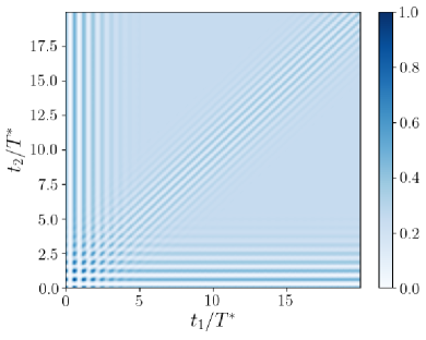
Figure 1: SCA of $G_{4}(t_{1},t_{1}+t_{2},t_{1})$, with an external magnetic field of $b_{x}=10$. It was averaged over $10^{6}$ Overhauser fields, determined from a Gaussian probability distribution.

Fig. 1 shows $G_{4}(t_{1},t_{1}+t_{2},t_{1})$ averaged over $10^{6}$ Gaussian distributed Overhauser fields. In this two dimensional color plot, the color encodes the magnitude of the correlation function. In the following, we will focus on two special lines in the $(t_{1},t_{2})$-plane: The diagonal defined by $t_{1}=t_{2}$ and the anti-diagonal for a fixed $T^{\prime}=t_{1}+t_{2}$. For these two cases, there exists published experimental data Bechtold et al. (2016).

a)

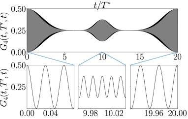
b)

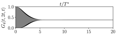
Figure 2: Cuts through the SCA (grey) of $G_{4}(t_{1},t_{1}+t_{2},t_{1})$ and the exact diagonalization (black) with $N=6$ $\frac{3}{2}$-spins and an external magnetic field $b_{x}=200$, averaged over $10^{6}$ Overhauser fields. a) shows the cut where the total time of measurement $t_{1}+t_{2}=T^{\prime}$ is a constant $T^{\prime}/T^{\ast}=20$. b) shows the cut where the pulses are equidistant, $t_{1}=t_{2}$.

In Fig. 2(a), the cut along the anti-diagonal direction, keeping $t_{1}+t_{2}=20T^{\ast}$ for $G_{4}(t,T^{\prime}=20T^{*},t)$ is depicted using both the SCA and the results of an full ED for the Hamiltonian $H_{\text{CSM}}$. For $t\approx 0$ and $t\approx T^{\prime}$, oscillations with a frequency of $\omega_{\text{L}}$ with a Gaussian envelope function can be seen, as plotted in the enlarged figures below.

In the middle, $t\approx T^{\prime}/2$, a frequency doubling with $\omega_{\text{L}}$, also characterized by a Gaussian envelope function with the same characteristic time scale $T^{*}$, is observed. The cause of this frequency doubling can be easily understood. In a finite external magnetic field, $G_{4}$ is reduced to $G_{4}(t,T^{\prime},t)\approx 1/4+2C_{4}(t,T^{\prime},t)$ according to Eq. (7) since $C_{2}(t)$ completely decays for $t\gg T^{*}$. For very strong external magnetic fields in the $x$-direction, we can additionally neglect the Overhauser field in leading order and obtain

$$C_{4}(t,T,t) = \frac{1}{16}\cos(2\omega_{\text{L}}(t-\frac{T^{\prime}}{2}))$$ (49)

from Eq. (V.1). Matching the Gaussian envelope of the ED results in fig. 2 to the results of Bechtold et al. Bechtold et al. (2016), we extracted the characteristic timescale as $T^{\ast}=1\,\mathrm{ns}$ which we used in all calculations as reference scale.

In the diagonal cut depicted in fig. 2(b), the correlation function oscillates with the Larmor frequency in the short-time range and quickly converges to a constant value of $3/8$ on the time scale $T^{*}$. Again, this can be understood by examining Eq. (7). Since $C_{2}(t)$ decays rapidly to zero, only $C_{4}(T^{\prime}/2,T^{\prime},T^{\prime}/2)=1/16$ is remaining according to (49) so that $G_{4}(t,2t,t)=3/8$ for $t\rightarrow\infty$.

Overall, the agreement of the SCA and the fully quantum mechanical ED with a rather small number of $N=6$ nuclear spins is remarkable in a larger external magnetic field, $|\vec{b}_{\rm ext}|\gg|\vec{b}_{N}|$. Finite size effects are small and responsible for the slight deviation of the ED envelop function compared to the Gaussian of the SCA, which is a static approximation for $N\to\infty$.

Apparently, the CSM Hamiltonian is not adequate for describing the long-time dynamics accurately. Bechtold et al. Bechtold et al. (2016) have reported that $G_{4}(t,2t,t)\to 1/4$ for $t\rightarrow\infty$ at moderate fields. In addition, there is a crossover reported to an exponential decay with long-time decay time $T_{2}\approx 1.4\,\upmu$s. Therefore additional interaction terms are required to cause the non-linear long-time dephasing effects observed in the experiment Bechtold et al. (2016), in particular for the case $t_{1}=t_{2}$, where the experiment reveals additional quantum effects.

To this end, we propose that by adding the nuclear-electric quadrupolar interaction as well as the nuclear Zeeman term to $H_{\text{CSM}}$ we are able to explain the experimental findings.

V.2 CSM with quadrupolar interaction

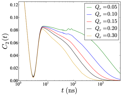
Figure 3: $C_{2}(t)$ computed by Lanczos method with restart with $N=9$ nuclear spins and no magnetic field. The strength of the quadrupolar interaction is varied to determine an experimentally relevant value of $Q_{r}$.

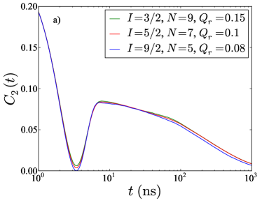
Figure 4: (a) $C_{2}(t)$ computed by Lanczos method with restart for different spin length $I=3/2,7/2,9/2$ and an adapted value of $Q_{r}$. The numbers of spins have been chosen to keep the Hilbert-space dimension almost identical. (b) $C_{2}(t)$ computed by Lanczos method with restart for two different values of $\alpha=0.5,1$ in (25) and $Q_{r}=0.1,0.15$ and $N=9$ nuclei with $I=3/2$. Parameters: $\vec{b}=0$.

Since $H_{\text{Z}}$ suppresses dephasing, we neglect this term and only investigate the influence of $H_{Q}$ at first.

V.2.1 The quadrupolar strength $Q_{r}$

The effect of $H_{Q}$ is determined by four parameters Bulutay (2012); Hackmann et al. (2015): (i) the overall quadrupolar strength $Q_{r}$, (ii) the distribution of the quadrupolar parameter $q_{k}$, (iii) the anisotropy $\eta$ and (iv) the distribution of the local nuclear easy axis all entering $H_{Q}$ defined in Eq. (26). For (ii)-(iv), we follow Refs. Bulutay (2012); Hackmann et al. (2015) by using the parameters stated in Sec. III.2 taken for a typical InGaAs QD.

By using the Lanczos approach with restart, we accurately calculated the long-time behavior of $C_{2}(t)$ under the influence of the quadrupolar interaction in the absence of an external magnetic field for a relatively large bath of $N$=9 nuclear spins with $I=3/2$. The time evolution is shown for five different values for $Q_{r}$ in fig. 3 on a logarithmic time scale up to $5\,\upmu$s. These Lanczos results reproduce the previous results obtained with Chebychev polynomial approach Hackmann et al. (2015). We matched theoretical curves for the spin-spin correlation function with the direct measurement of $C_{2}$ Bechtold et al. (2015) and extracted $Q_{r}\approx 0.15$ for making contact to the experiment. This value is very close in magnitude to the parameter used in Ref. Glasenapp et al. (2016) to explain spin-noise data obtained on different InGaAs QD samples.

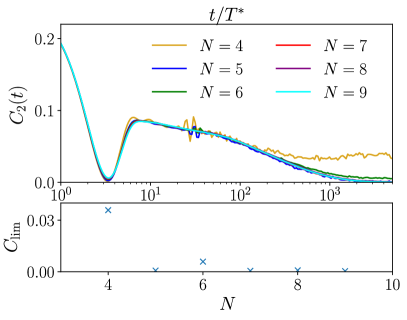
Figure 5: $C_{2}(t)$ with a quadrupolar coupling strength of $Q_{r}=0.15$, no magnetic field and a varying number of nuclear spins. The long time limit shows an even-odd behavior in regard to bath size, as shown in the lower figure.

In order to determine the finite size effects of our small nuclear spin bath, we compare $C_{2}(t)$ for different bath sizes and a fixed quadrupolar coupling of $Q_{r}=0.15$. The top panel of fig. 5 demonstrated the fast convergence of $C_{2}(t)$ with $N$. While $C_{2}(t)$ can be calculated exactly for as large as $N=9$ with a Lanczos method with restart without any problem, this is impossible for $C_{4}$ due to the scaling of the nested Lanczos algorithm with the exponential growth of the Hilbert space with $N$. A finite size analysis for $C_{\rm lim}=C_{2}(t\to\infty)$ is depicted in the lower panel of fig. 5. Clearly visible are even-odd oscillations which approach $C_{\rm lim}=0$ at large $N$ within a numerical error of $\mathcal{O}(10^{-4})$. In order to minimize the finite size effect in the long time limit, we restrict ourselves to odd bath sizes in all following simulations.

Fig. 4(a) illustrates the influence of the spin length $I$ on $C_{2}(t)$. The data for $I=3/2$ has been taken from Fig. 3. When adjusting the relative coupling strength $Q_{r}$ for each $I$ appropriately, we can obtain a universal curve for $C_{2}(t)$. The small differences in the minimum are well understood Stanek et al. (2013); Hackmann (2015) and are related to the number of spins. This illustrates that the additional dephasing is driven by presence of $H_{Q}$ while the differences in the spin length are insignificant.

The marginal influence of the choice of $\alpha$ in eq. (25) is depicted in fig. 4(b). At intermediate times, small deviations are observable, but the long time limit is not effected and fully determined by the value of $Q_{r}$.

V.2.2 Influence of $H_{Q}$ on $G_{4}$

Fig. 6 shows $G_{4}(t,2t,t)$ with a quadrupolar interaction strength $Q_{r}=0.15$. With this quadrupolar interaction strength, $G_{4}(t,2t,t)$ rather rapidly approaches a constant, augmented with some finite-size oscillations. As depicted in the inset of fig. 6, this decay occurs one a time scale of approximately 10 ns. The decay is not influenced significantly by the externally applied magnetic field as long as the magnetic field exceeds $b_{x}=50$. The long-time exponential decay reported in the experiment Bechtold et al. (2016) is absent in our calculations.

To suppress finite-size oscillations in favor of showcasing the long-time behavior, we smooth the curves through convolution with a Gaussian function

$$g(t)=\frac{1}{\sqrt{2\pi\sigma^{2}}}\exp{\left(-\frac{t^{2}}{2\sigma^{2}}\right)}.$$ (50)

In both fig. 6 as well as fig. 7, a standard deviation $\sigma=60\,\text{ns}$ was used for this low-pass filter. This is sufficiently small to not distort the curve progression in $\mathcal{O}(\upmu\mathrm{s})$.

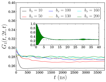
Figure 6: $G_{4}(t,2t,t)$ as function of $t$ for different external magnetic fields. The curves were smoothed through a low-pass filter to suppress finite size oscillations. The inset reveals the short-time behavior without the low-pass filter. One can see that $G_{4}$ decays down to a constant level close to 1/4 in $\mathcal{O}(\text{ns})$, and that the time frame of the decay is not dependent on the applied magnetic field. Parameters: $N=5$ with $I=\frac{3}{2}$ and $Q_{r}=0.15$.

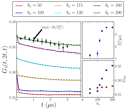
Figure 7: $G_{4}(t,2t,t)$ as function of $t$ for different external magnetic fields. and a relative strength of the Zeeman splitting of $z=1/800$. The decoherence time $T^{\text{G}}_{2}$ and the convergence level $G_{\text{lim}}$ are plotted against the external magnetic field $b_{x}$. A low pass filter was utilized to suppress finite size oscillations. $G_{4}(t,2t,t)$ obtained by a Lanczos algorithm and a bath size of $N=7$ and $b_{x}=200$ is shown in black dots. In the upper right panel , the decay time $T^{\text{G}}_{2}$ is plotted in blue dots. The long-time limit $G_{\text{lim}}$ is shown in the lower right. The blue and red squares denote $G_{\text{lim}}$ for $z=1/800$ and $G_{\text{lim}}$ for $z=0$, respectively. The dashed lines show the ED data fitted with eqn. (52). Parameters: $N=5$ with $I=\frac{3}{2}$ and $Q_{r}=0.15$.

V.3 Combining $H_{\rm CSM}$ with quadrupolar interaction and Zeeman splitting of the nuclei

In order to make a connection to the experiments Bechtold et al. (2016), a suppression of the additional long-time dephasing mechanism introduced by $H_{Q}$ is needed. This effect is provided by the nuclear Zeeman term, which dominates the local nuclear spin dynamics at large external magnetic fields: The Zeeman splitting of the nuclei suppresses nuclear spin flip processes once the nuclear Zeeman energy is within the order of magnitude of the hyperfine interaction.

To this end, we consider the full Hamiltonian $H=H_{\text{CSM}}+H_{Q}+H_{\text{Z}}$ in this section. With this additional term, a completely different behavior for the long-time limit of $w(t,t)=G_{4}(t,2t,t)$ emerges as depicted in fig. 7. In the larger left panel of the figure, $G_{4}(t,2t,t)$ is plotted up to 4$\,\upmu$s for various magnetic field strengths, again using the low-pass filter to suppress the finite size noise in the long time evolution. Setting $g=0.55$ for the electron spin in a QD, and the time scale $T^{*}=1\,$ns, the dimensionless fields $b_{x}=50,100,115,130,160,200$ translate to physical units of $B_{x}=|\vec{B}_{\rm ext}|=1.03,2.07,2.38,2.68,3.31,4.14\,$T. All curves are calculated using ED with only $N=5$ nuclear $3/2$-spins, a uniform average ratio $z=1/800$ and averaged over $N_{C}=32$ configurations of $\{A_{k}\}$.

For low magnetic fields $b_{x}=50,100$, the results are very similar to the results without $H_{Z}$ depicted in fig. 6. Rather rapidly, $G_{4}(t,2t,t)$ decays to its asymptotic magnetic field dependent long time limit defined as

$$G_{\text{lim}}(b_{x})=\lim_{t\rightarrow\infty}G_{4}(t,2t,t).$$ (51)

Here, however $G_{\text{lim}}(b_{x}=50)$ is lower than the value without nuclear Zeeman term, indicating that for small and intermediate fields the non-linear nuclear dynamics governed by the combination of the nuclear Zeeman term and nuclear quadrupolar interaction yields an overall long time decay closer to the theoretical lower limit of $1/4$ for a complete dephasing of the fourth-order spin correlation functions $C_{4}(t,2t,t)$.

$G_{\text{lim}}(b_{x})$ is shown as red squares for $H=H_{\text{CSM}}+H_{Q}$ and as blue squares for the full Hamiltonian in the lower right panel of fig. 7. A qualitatively different picture emerges once $b_{x}$ exceeds $100$. While $G_{\text{lim}}$ remains almost magnetic field independent for $H_{\text{CSM}}+H_{Q}$, $G_{\text{lim}}(b_{\rm ext})$ monotonically increases with $b_{x}$ for the full Hamiltonian, as plotted in the lower right panel of fig. 7. The increase occurs rather rapidly and approaches a plateau for large fields, since $G_{\text{lim}}(b_{x})$ cannot exceed the asymptotic value $3/8$ bound by the SCA.

We have analyzed the slow long-time decay of $G_{4}(t,2t,t)$ by assuming an exponential form

$$G_{4}(t,2t,t)=G_{\text{lim}}(b_{x})+\xi\exp(-2t/T^{\mathrm{G}}_{2})$$ (52)

parametrized by the amplitude $\xi$ and the additional decoherence time $T^{\mathrm{G}}_{2}$ in order to connect to the experimental findings by Bechtold et al. Bechtold et al. (2016). These fits are added as dashed lines to the calculated $G_{4}(t,2t,t)$ in the left panel of fig. 7. The decoherence time $T^{\mathrm{G}}_{2}$ obtained by this fit is plotted as function of the external magnetic field in the upper right panel of fig. 7. $T^{\mathrm{G}}_{2}$ is small and difficult to determine for small fields and rapidly increases around $b_{x}=115$ being equivalent to $B_{x}=2.38\,$T. This is in full accordance with Ref.  Bechtold et al. (2016) where only the data for largest field value of $B=4\,$T was fitted with an exponential form. While we find values of $T^{\mathrm{G}}_{2}\approx 3.5\upmu$s at $B_{x}=4.14\,$T by Bechtold et al. reported $T^{\mathrm{G}}_{2}=1.4\pm 0.1\,\upmu\text{s}$ at an external magnetic field of $B_{x}=4\,$T. Note that the experimental data points presented in Fig. 4(a) of Ref.  Bechtold et al. (2016) can also be fitted with a larger $T^{\mathrm{G}}_{2}$, if one only considers the data points for the long time decay $t>300\,$ns. $T^{\mathrm{G}}_{2}$ between $2-5\,\upmu$s can be obtained, indicating that the values for $T^{\mathrm{G}}_{2}$ strongly depended to the fit procedure.

In order to estimate the finite-size effects, we have calculated the long-time dynamics of $G_{4}(t,2t,t)$ for $N=7$ nuclear spins using the numerically expensive Lanczos approach with restart outlined in Sec. IV.3: The larger the external magnetic field, the larger the number of spins, the larger the spectrum of $H$, the shorter the time evolution step will be for a given Krylov space dimension $M$. We typically used $M=400$ and a propagation time of $\Delta t=2\,$ns for a single step. Since the calculation required two-week runs on our HPC cluster, we have evaluated $G_{4}(t,2t,t)$ only at a set of discrete data points for the largest magnetic field $b=200$.

Within the finite size errors, the Lanczos data for $N=7$ are identical to the results obtained from the ED for $N=5$, leading to the conclusion that the long-time scale extracted from the ED does not contain substantial finite size errors for a small increase of $N$. However, we are aware that the limitation of the energy spectrum of the Hamiltonian introduces finite-size errors which will influence $G_{\text{lim}}(b_{x})$. In the real system, the nearly continuous distribution function $P(A)$ of the hyperfine coupling will lead to a nearly continuous spectrum of the Hamiltonian so that phase space for spin-flip processes with be larger, and we expect that long-time limit $G_{\text{lim}}(b_{x})$ will be smaller than in our case. We have demonstrated that effect for $C_{2}(t)$ calculated with the full model in fig. 5: The finite size offset of $C_{2}(t\to\infty)$ depicted in the lower panel of fig. 5 suggests that a complete decay of $C_{2}$ can only be achieved in the limit $N\to\infty$.

Since finite-size corrections to asymptotic limit $G_{\text{lim}}(b_{x})$ will only influence prefactor $\xi$, the exponential decay time $T_{2}$ should be unaltered. We conclude that our findings for $T^{\mathrm{G}}_{2}$ agree not only qualitatively but also quantitatively with the experiments.

V.4 Spin echo experiments modeled with the full Hamiltonian

We derived in section II.2 that the amplitude of the spin echo measured by Press et al. Press et al. (2010) can be described as a fourth-order correlation function $P_{g_{0},g_{0}}(T,\tau)$. To properly compare our results with the experimental measurements, we study both $P_{g_{0},g_{0}}(T=\text{const},\tau)$ as a function of $\tau$ and the oscillation amplitude of $P_{g_{0},g_{0}}(T,\tau=0)=\bar{P}_{g_{0},g_{0}}(T)$ as a function of $T$ for several external magnetic fields. Similarly to $G_{4}(t,2t,t)$ measured in the Bechtold et al. experiment Bechtold et al. (2016), the amplitude of $P_{g_{0},g_{0}}(T,\tau)$ exhibits a long time exponential decay

$$\bar{P}_{g_{0},g_{0}}(T)=P_{\text{lim}}+\zeta\exp{\left(-\frac{2T}{T^{\text{P}}_{2}}\right)}.$$ (53)

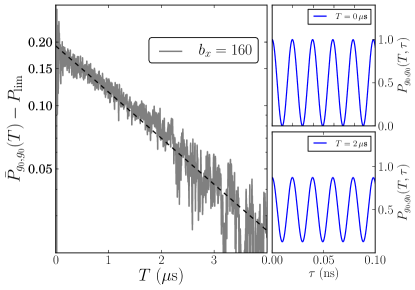
Figure 8: Left panel: Exponential decay of the amplitude of $P_{g_{0},g_{0}}(T,\tau=0)$ with $N=5$, here plotted for $b_{x}=160$ on a log scale, which corresponds Press et al. (2010) to a magnetic field $B_{x}=4.11\,$T for $g_{\text{e}}=0.442$. The decay time was fitted as $T_{2}^{\mathrm{P}}=3.96\,\upmu$s. On the right hand side, $P_{g_{0},g_{0}}(T,\tau)$ for a constant pulse distance $T$ is shown, once for $T=0\,\upmu$s and once for $T=2\,\upmu$s. The spin echo oscillates with twice the Larmor frequency, like $G_{4}(t,T,t)$ at $t\approx T/2$. All system parameters are equal to the ones used in fig. 7 to describe the experiment by Bechtold et al. Bechtold et al. (2016).

For the computation of $P_{g_{0},g_{0}}(T,\tau)$ using ED, the same system parameters were employed as for the computation of $G_{4}(t,2t,t)$ in fig. 7. If $T$ is kept constant, $P_{g_{0},g_{0}}(T,\tau)$ oscillates with twice the Larmor frequency as function of $\tau$. This can be understood analytically: When neglecting the Overhauser field, one again obtains

$$P_{g_{0},g_{0}}(T,\tau)=\frac{1}{2}+\frac{1}{2}\cos(2\omega_{\text{L}}\tau).$$ (54)

The decay of this coherent oscillations of the electron spin in the external magnetic field observed in the experiment Press et al. (2010) is also caused by the interaction of the electron spin with the surrounding nuclear spins.

When computing $P_{g_{0},g_{0}}(T,\tau)$ with ED using the full Hamiltonian, the decay of the spin-echo amplitude is evident, though not as pronounced as in the experiment. Exponential fitting shows that the decay time $T_{2}$ is similar, but that in our theoretical model the long-time limit of the probability, $P_{\text{lim}}=\lim_{T\to\infty}P_{g_{0},g_{0}}(T,0)$, lies above the experimental values. The coherent oscillations in $\tau$ are depicted for two different fixed times $T$ in the right panel of fig. 8. By applying the pulse sequence of $\pi/2-\pi-\pi/2$-pulses long time coherence can be maintained on a time scale of $T^{\text{P}}_{2}\gg T^{*}$. We have extracted $T_{2}^{\text{P}}$ as function of the applied external magnetic field shown in fig. 9. The calculated functional dependence of $T^{\text{P}}_{2}\gg T^{*}$ on the external magnetic field agrees remarkably well with the experimental data of fig. 4 in ref. Press et al. (2010).

Although $P_{g_{0},g_{0}}(T,\tau)$ behaves very similar $G_{4}(t_{1},t_{1}+t_{2},t_{1})$ when identifying $t_{1}=T+\tau$ and $t_{2}=T-\tau$, the magnetic field dependency of the two long-time scales $T^{\text{G}}_{2}$ and $T^{\text{P}}_{2}$ differs as well as their saturation values, $T^{\text{P}}_{2}\approx 4\,\upmu$s and $T^{\text{G}}_{2}\approx 3.5\,\upmu$s respectively. This agrees excellently with the experiments, where the $T^{\text{P}}_{2}$ measured by spin-echo method Press et al. (2010) was also higher than the $T^{\mathrm{G}}_{2}$ obtained by the three measurement pulse experiment Bechtold et al. (2016). We attribute the different in the long-time scales by the difference of the two different fourth-order spin correlation functions measured in the different experimental setups: While Bechtold et al. have focused on measuring only $S_{z}$, the $\pi/2$ pulse connect both spin components $S_{z}$ and $S_{y}$ orthogonal to the applied external magnetic field, see eqs. (7) and (17). Note that the underlying dynamics and all model parameters have been identical in our calculations for both correlation functions.

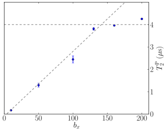
Figure 9: The decay time $T^{\text{P}}_{2}$ of $\bar{P}_{g_{0},g_{0}}(T)$ dependent on the external magnetic field $B_{x}$. The grey dashed lines are guides to the eye, indicating a rising slope that saturates at magnetic fields $b_{x}>130$. With $g_{\text{e}}=0.442$ the saturation point is reached at $B_{x}\geq 3.5\,$T with a saturation level of $T^{\mathrm{P}}_{2}\approx 4\,\upmu$s. A higher saturation point $B_{x}=4\,$T at a lower saturation level $T^{\mathrm{P}}_{2}\approx 3\,\upmu$s was reported by Press et al. Press et al. (2010).

VI Summary and conclusion

We have shown that the joint probability $w(t_{1},t_{2})$ of measuring a central spin $\ket{\downarrow}$ twice at times $t_{1}$ and $t_{1}+t_{2}$ in a quantum dot after preparing the central spin in a spin $\ket{\downarrow}$ state is related to the fourth-order correlation function $w(t_{1},t_{2})=G_{4}(t_{1},t_{1}+t_{2},t_{1})$. $G_{4}$ was computed via the SCA, the ED and and the Lanczos algorithm. To determine the influence of the different interactions, we have studied the long time behavior of $G_{4}$ with and without nuclear Zeeman splitting and quadrupolar interaction, and have compared the results to the experimental findings reported by Bechtold et al. Bechtold et al. (2016, 2015). $w(t,t)$ exhibits a long time exponential decay in a strong transversal magnetic field for equidistant probe pulses $(t_{1}=t_{2})$, which cannot be understood with the semi-classical approximation or the full quantum dynamics of the CSM including electron and nuclear Zeeman term.

By including the nuclear-electric quadrupolar interaction in the full-time reversal form Slichter (1996); Bulutay (2012); Hackmann et al. (2015); Glasenapp et al. (2016) as well as nuclear Zeeman term, for the CSM, the ED produces results which concur qualitatively with the findings of the recent experiments Bechtold et al. (2016, 2015). We have used the spin-correlation function $C_{2}(t)$ to determine $T^{*}$ and the relative quadrupolar coupling strength $Q_{r}$ relevant for connection to the experiment. $G_{4}$ computed using ED for the simple CSM model including only electron Zeeman splitting is very similar to $G_{4}$ computed by the SCA: Both approaches perfectly agree in short-time behavior but lack to explain the experimentally observed long-time decay of the correlation function. Adding the nuclear quadrupolar coupling to the Hamiltonian and neglecting the nuclear Zeeman term introduces a rapid decay of $G_{4}(t,2t,t)$ after the initial coherent Larmor oscillations on a time scale of $t_{\rm decay}\approx 10\,$ns. We have demonstrated that the nuclear Zeeman interaction is essential to observe the crossover from a fast non-exponential decay caused by the nuclear quadrupolar coupling in weak and intermediate magnetic field to a slow exponential decay at larger magnetic field. Above a threshold of $b_{x}\approx 100$, $G_{4}(t,2t,t)$ exhibits a long-time exponential decay dependent on the field strength, with a plateauing characteristic time scale $T_{2}=3.5\,\upmu$s. With the full model, the increasing external transversal magnetic field $b_{x}$ leads to a monotonically increasing asymptotic limit $G_{\text{lim}}(b_{x})$. Our findings agree with the experimental results reported by Bechtold et al. Bechtold et al. (2016).

The intrinsic dephasing time $T_{2}$ was also measured through the spin echo method by Press et al. Press et al. (2010). We were able to show that the spin echo measurement is described by a fourth-order spin correlation function $P_{g_{0},g_{0}}(T,\tau)$ that is different from $G_{4}$, involving $S_{y}$ and $S_{z}$. The decay mechanisms are the same, and the long time behavior is qualitatively similar. Both $P_{g_{0},g_{0}}$ and $G_{4}$ reach an asymptotic value for the decay time $T_{2}$ at large external magnetic fields. The asymptotic decay time of $P_{g_{0},g_{0}}$ is higher, $T^{P}_{2}=4\,\upmu$s, than that of $G_{4}$, where we have found $T_{2}^{\mathrm{G}}=3.5\,\upmu$s. This concurs with the experiments, since Press et al. also reported a higher asymptotic decay time $T_{2}^{\mathrm{P}}=3\,\upmu$s Press et al. (2010) than Bechtold el al. Bechtold et al. (2016), who measured $T_{2}^{\mathrm{G}}=1.4\,\upmu$s for $B_{x}=4\,$T. However, the approach of the asymptotic value for large magnetic fields significantly differs for the two fourth-order correlation functions. While the $T_{2}^{\text{P}}$ shows a slow linear rise – see also fig. 9 – that agrees very well with the experiment, $T_{2}^{\text{G}}$ exhibits a threshold behavior with a rapid rise at $b_{x}\approx 100$.

For the anti-diagonal of $w(t_{1},t_{2})$ defined by the fixed distance of the second probe pulse with respect to the initial pump pulse ($t_{1}+t_{2}=T^{\prime}$), i. e. $G_{4}(t_{1},T^{\prime},t_{1})$ both SCA and ED show $G_{4}$ oscillating with twice the Larmor frequency and a Gaussian envelope around $t_{1}=T^{\prime}/2$. The cause of the frequency doubling can be analytically understood by neglecting the Overhauser field compared to a strong transversal magnetic field in zero order while the Gaussian enveloped is caused by the dephasing introduced by the Overhauser field. The same behavior is also observed in $P_{g_{0},g_{0}}(T,\tau)$ at constant $T$.

In conclusion, the CSM model augmented with the nuclear-electric quadrupolar coupling and nuclear Zeeman splitting is an adequate description for fourth-order correlation functions in QD. While quadrupolar coupling induces an additional decay of the correlation functions towards universal constants, a increasing nuclear Zeeman splitting suppresses this effect leading to a long-time exponential decay. Applying the full model predicts a long-time exponential decay of the fourth-order correlation function at high transversal magnetic fields that qualitatively and quantitative agrees with the recent experimental results.