Proof of Concept of Wireless TERS Monitoring

Abstract

Temporary earth retaining structures (TERS) help prevent collapse during construction excavation. To ensure that these structures are operating within design specifications, load forces on supports must be monitored. Current monitoring approaches are expensive, sparse, off-line, and thus difficult to integrate into predictive models. This work aims to show that wirelessly connected battery powered sensors are feasible, practical, and have similar accuracy to existing sensor systems. We present the design and validation of ReStructure, an end-to-end prototype wireless sensor network for collection, communication, and aggregation of strain data. ReStructure was validated through a six months deployment on a real-life excavation site with all but one node producing valid and accurate strain measurements at higher frequency than existing ones. These results and the lessons learnt provide the basis for future widespread wireless TERS monitoring that increase measurement density and integrate closely with predictive models to provide timely alerts of damage or potential failure.

1 Introduction

Underground construction of subway stations and building basements are frequently accomplished through ‘bottom-up’ methods; where the permanent structure is built within an excavation pit that is supported by a Temporary Earth Retaining System (TERS). Typically TERS comprise of perimeter walls that are supported internally by cross-lot bracing struts, or externally by tieback anchors (installed in the adjacent ground). These temporary structures are designed to support the loads exerted by the retained soil mass (including pore water pressures), forces induced by foundations from adjacent buildings, etc. Numerical analyses of soil-structure interactions (usually by finite element methods) are used to predict the performance of the structure including the loads in the structural elements, magnitudes of wall deflections and ground deformations at all stages of the construction process. During construction, TERS systems are extensively monitored to ensure the stability of the works and to control/mitigate impacts of excavation-induced ground movements that can affect adjacent structures and facilities. Field monitoring typically includes measurements of compression forces in the strutting system (via strain gauges or load cells), deflections (and flexure) of the retaining wall (via inclinometers), surface and subsurface ground movements (optical surveys, inclinometers and extensometers) and pore water pressures (piezometers). In current practice, the monitoring data are primarily used to i) compare against the expected values predicted by prior analyses of soil-structure interaction, to determine if the design specification has been exceeded and ii) trigger static threshold based flags/alarms. The high unit costs for installing these instruments (particularly subsurface sensors) leads to sparse spatial coverage at most construction sites. Furthermore, there is little use of the data to interpret the actual field performance and hence, to update model predictions and reduce risks associated with the construction process.

Wireless sensing offers an attractive alternate approach for monitoring structural performance. By reducing the unit cost of sensor installation, wireless sensor networks can increase the spatial and temporal resolution for measuring forces in the bracing system (compared to wired devices).

The goal of this research is to enable robust, reliable wireless collection of strain measurements in an excavation environment and make it available for on-line integration, in real-time, with a user application. This paper demonstrates:

• the feasibility of using Wireless Sensor Networks (WSNs) for TERS. An end-to-end proof-of-concept system (ReStructure) has been developed and deployed on an excavation site (alongside a conventional wired system, where forces were monitored by vibrating wire strain gauges, done by a specialist instrumentation contractor) to acquire, transmit and aggregate strain data. Criteria used for evaluating the suitability of the prototype for the application have been: i) the validity and accuracy of the measurements against the industry gold-standard systems, ii) wireless communication reliability and data yield, iii) system survivability in field, and iv) system and battery life.

• The paper provides insights into the feasibility of large scale, low cost intelligent WSNs monitoring for TERS through analysis of the data archive created through the pilot deployment. Lessons are drawn from the system design, implementation and deployment that add to the existing body of knowledge on deployable WSNs for structural monitoring.

In this paper we review the current literature (Section 6) on related wireless systems for structural health monitoring. We then discuss the design specifications for the current application to Temporary Earth Retaining systems (Section 2), and present details of the prototype design and implementation (Section 3). We review data from two relatively short-duration field deployments (Section 4) and the lessons learned from this experience (Section 5).

2 ReStructure: design specification and model integration

The goal of ReStructure is to enable collection of strain measurements in an excavation environment and make it available for on-line integration, in real-time, with a user application. Figure 1 presents the system architecture.

Figure 1: The ReStructure system architecture involves wireless strain sensors transmitting their data locally to a gateway that then forwards via 3G to a server. The server can then be used to display or possibly to integrate with a finite element (FE) model.

2.1 The WSN design specification

The design specification for the WSN was developed to meet a variety of constraints associated with the expected physical loads (strains), project duration, sampling rate and unit costs of the sensor nodes.The following generic requirements were defined at the outset:

Data acquisition and wireless communication

The sensor network is expected to collect and transmit data at 5 minute intervals. The nodes are powered via batteries.

Measurement parameters

The primary measurand is strain (as a proxy for compressive load in the cross-lot bracing struts). Traditionally, strain is measured using vibrating wire gauges or resistive foil gauges. In commercial structural engineering projects, the standard is to use vibrating wire gauges that are sampled at hourly intervals (or less frequently) and have been shown to provide stable measurements over long-term deployments in harsh environmental conditions. The current deployment uses resistive foil gauges. These provide a small form factor, have much lower unit costs and simpler field installation (attachment by spot welding) but raise concerns about long term drift in the measurements.. Environmental air temperature and humidity are also measured in the proximity of the strain gauges in order to compensate for environmental effects. The current application uses a single strain gauge for axial compression of the strut (and assumes that bending strains are negligible).

Target lifetime

The sensor network is intended to last for the lifetime of an excavation (approximately 1 year). Individual nodes are to be added to the network as the excavation progresses.

Packaging and deployment

The strain gauges are mounted directly on the struts. Sensor nodes must be attached close to the foil gauges to reduce lead length and help protect the gauges. It is intended for sensor nodes to be i) low cost to enable dense deployments and ii) small in size and robust to prevent them being destroyed or stolen during operation.

There are a number of challenges associated with devising a system that fulfils this set of requirements:

1. maintaining an evolving and growing network in a climatically harsh and dynamic construction environment

2. meeting the system target life in face of environmental obstructions (i.e, where transmission retries penalise the energy consumption)

3. ensuring sufficiently high data yield to enable its use in models and user applications

4. ensuring adequate measurement accuracy with low cost sensing devices

The lack of opportunity to retrieve and debug or otherwise access nodes after installation is an added constraint and one that hindered learning from node failure events.

3 ReStructure: implementation and prototype characterisation

To reduce risk and development time, the implementation was based on off-the-shelf hardware and software wherever possible. A number of custom hardware interfaces and software components were developed in-house as specified below. The node and gateway energy profiling and the network coverage / yield characterisation performed show the alignment with the design requirements and open areas for further work.

3.1 Sensor node

The sensor node (shown in Figure 2) combines the Zolertia Z1 (MSP430 CPU and a CC2420 radio) platform with a custom strain gauge PCB. The custom PCB supports one bonded foil strain gauge whose readings are acquired using a Wheatstone bridge combined with a low power 16-bit ADC (TI ADS1115). Measurement resolution is $<1\,\mathrm{\mu{}e}$ with a measurement range of $\pm 2\,500\,\mathrm{\mu{}e}$. External temperature/humidity monitoring is enabled by a Sensirion SHT15. Each sensor node is packaged in an IP65 aluminium enclosure ($115\times 65.5\times 50\,\mathrm{mm}$, $370\,\mathrm{g}$) with holes for an external radio antenna ($4.4\,\mathrm{dBi}$ Antenova Titanis), a cable gland for the strain gauge wiring, and a waterproof breathable membrane for the SHT15. Magnetic feet on the enclosures allow the nodes to be placed on the strut without welding. A deployed sensor node is shown in Figure 7.

The node’s software was developed using Contiki WSN OS, which provides a network stack with a low power MAC (ContikiMAC) and multi-hop tree formation and data collection protocol (Contiki Collect). We reduced the size of the recent message buffer kept by each node to minimise the time taken to verify network formation after a node restart. Custom drivers were written for the strain interface board.

At application level, a traditional sense and send system was implemented that acquires, stores to flash, and transmits network information (time, RSSI, beacon interval, sequence number, neighbours) as well as a single strain and temperature/humidity measurement at 5 minute intervals (92 bytes of payload total). Storing samples to flash means that, even if the network fails, all measurements will be recorded while the node has sufficient battery power. Oscilloscope–based energy profiling was used to estimate the lifetime of the sensor nodes given a particular battery capacity and sampling rate [2].

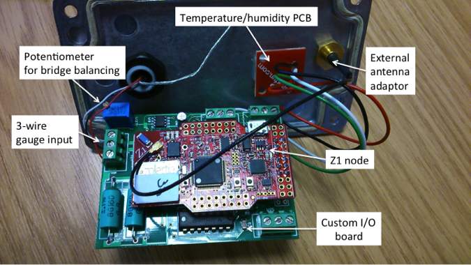
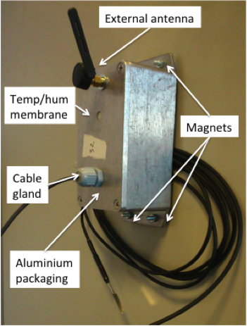
Figure 2: ReStructure wireless sensor node hardware

3.2 Gateway

The Gateway was built using a Raspberry Pi model A+ combined with a TelosB node and a USB 3G modem (both with external antennas). The Gateway is deployed inside an IP65 mild steel enclosure and mounted on a pole. Due to deployment constraints, the Gateway was powered by a $12\,\mathrm{V}$ $100\,\mathrm{Ah}$ battery (Figure 3). During normal operation WSN data is collected by the TelosB, aggregated at the Raspberry Pi and transmitted hourly via 3G to a remote server (and subsequently, compared with the FE model).

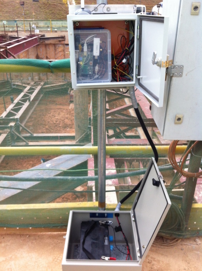
Figure 3: Deployment of server at the construction site, nodes are placed at the second strut level (approx. $12\,\mathrm{m}$ away)

Based on prior experience with deploying WSNs, the Gateway design and implementation focused on:

• minimising power consumption—by disabling HDMI on the Raspberry Pi and devising custom circuitry to allow the power to the TelosB and 3G modem to be controlled through GPIOs so that it can be turned on only when needed.

• improving fault tolerance between the TelosB and the Raspberry Pi to minimise on-site maintenance—by devising a simple handshake connection so that the Raspberry Pi can periodically check and restart the TelosB if necessary. For 3G transmissions, if an hourly update fails, it is rolled into the following hour’s transmissions, and data is always archived locally in case of extended 3G outages.

• ensuring on-site deployment, debugging and maintenance are as easy as possible—the Gateway can host a USB WI-FI dongle. When the dongle is connected, the Gateway becomes a wireless access point (using hostap [22]), hosting a web page that shows real-time updates of data. Our measures reduced the average power requirement of the gateway from over $4.8\,\mathrm{W}$ to $1.5\,\mathrm{W}$.

Based on gateway micro-benchmarking tests, we estimate that a $100\,\mathrm{Ah}$ battery will provide one month’s operation (details in Section 3.3)

3.3 Energy consumption benchmarking

Node Energy

Benchmark measurements were conducted for the node operations and used to predict lifetime based on $2\times\mathrm{AA}$ batteries. Power was estimated by measuring the voltage drop over a shunt resistor on the ground line of the power supply. The power consumption for the following operations was determined:

• sense/sample strain only (no warm up time on bridge)

• sense/sample strain and temp/humidity

• sense/sample strain and write data to flash storage

• sense/sample strain and send data over network

• idle (no sampling, listening for packets)

Figure 4 shows a typical power use profile when switching on strain bridge and taking a sample. Each point on the graph is an average of 64 oscilloscope samples. Based on these measurements, we derived Table 1, which shows an estimated breakdown of power consumption by operation.

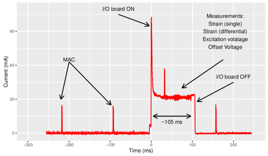
Figure 4: The characteristic current consumption when switching on strain bridge and taking a sample. Note that this profile does not include time spent to ‘warm-up’ the bridge, i.e. ensure that the strain value has reached a stable reading before taking a measurement.

Table 1: Micro-benchmark estimates for a ReStructure node running sense-and-send. The average current, for all but Idle, excludes the idle current.

Process	Duration (ms)	Average current (mA)	mW
Warm up bridge	$5\,000$	$33.6-1$	$1.63$
Strain sample	$105$	$33.6-1$	$0.034$
Temp/humidity sample	$315$	$33.6-1$	$0.1$
Write data to flash	$8$	$6.7-1$	$0.000\,46$
Send message	$30$	$17.9-1$	$0.005\,1$
Idle	$300\,000$	$1$	$3$
Total			$4.8$

The energy benchmarking results in Table 1 provide a profile of the design and help to identify opportunities for improvement. Note that the time taken to sample temperature and humidity is almost three times the time taken to acquire the strain measurements. Because the I/O board controls the temperature/humidity sensor’s power, the Wheatstone bridge is also powered during this time. A refinement of the PCB design may add an extra switch to allow the Wheatstone bridge to be powered independently of the temperature/humidity sensor.

The individual operations of a sensing cycle (5 minute interval) were measured and aggregated to determine a simple, best–case baseline for node lifetime of 205 days of operation with $2\times 7.8\,\mathrm{Ah}\times 1.5\,\mathrm{V}$ C-cells.

Gateway

Table 2 shows an estimated breakdown of power consumption by functionality. Using a $12\,\mathrm{V}$ $100\,\mathrm{Ah}$ car battery we estimate the gateway life to be 31 days. Future designs should consider making use of solar panels.

Table 2: Micro-benchmark estimates for the ReStructure gateway.

Process	Duration (s)	Average energy (A)	As
3G data transmission	60	0.27	16.2
Plotting	60	0.13	7.8
Processing	3480	0.126	438.48
Total	3600		462.48

3.4 Network performance

The multi-hop network characterisation below provides insights into the performance and yield expected from the ReStructure prototype in a heavy machinery environment (see Figure 5) but without the harsh climatic conditions of the construction site. Over a series of tests, each of the nodes transmitted ‘dummy’ measurement packets at 5 minutes interval.

Figure 5: Approximate layout of nodes during network test. Arrows indicate antenna orientation; the sink is located roughly 3m to the left of node A.

Table 3 provides a summary of the performance of the network over a (roughly) 23 hour test (transmitting about 276 packets). The performance is summarised by two measures, Packet Delivery Ratio (PDR) and Link Stability. PDR is the percentage of packets received vs. expected. We define link stability as the proportion of time that nodes are sending beacons at the longest interval ($3600\,\mathrm{s}$). Collection tree protocols, such as Contiki Collect, broadcast fewer beacon messages when the network is stable [6]. In addition, the number of packets sent directly to the sink node versus other nodes is recorded to identify the proportional use of direct versus multi-hop transmission.

Table 3: Summary of network statistics from 1-day multi-hop network deployment.

Node	Duration (h)	PDR (%)	Link stability	Most common	MCP (%)
			(%)	parent
A	22.7	91.5	1.6	Sink	57.8
B	22.8	100.0	94.5	Sink	100.0
C	22.7	89.3	2.1	Sink	70.0
D	22.6	100.0	94.6	Sink	100.0

Over the testing period, we observed two stable network connections, with 100% PDR, that were directly connected to the sink (Nodes B and D), and two unstable network connections (Nodes A and C) that had a lower PDR, were sending through two or more hops, and were changing path frequently. This test indicates that that data yield and network stability are related and that if stability is low, data yield will also be low.

4 Field deployment

The prototype ReStructure system was deployed to monitor axial strains for a series of selected struts within a large excavation pit. Data was collected between May and December 2015. The deployment environment was particularly challenging, due to:

• Climate - The site is located in a tropical climate with frequent and severe rainstorms. Temperatures can rise to $35\,\textrm{\textcelsius}$ and 99% RH above ground, and above $40\,\textrm{\textcelsius}$ inside the excavation. There are large daily cycles where temperature can change by $24\,\textrm{\textcelsius}$ and relative humidity by 60%. Temperature and thus thermal expansion affects both the TERS and the strain gauges. In addition, strain gauges are subject to apparent strain, a change in resistance that is not due to a loading change in the strut, but is related to the differences in thermal expansion coefficient between the strain gauge and strut being monitored.

• Obstructions - Radio channel quality was expected to be low due to the construction environment, which is mainly a combination of metal and concrete materials that can reflect and attenuate radio signals. The construction site itself is very dusty and there is lots of machinery and movement that could damage equipment. This was expected to affect the packet delivery radio (data yield), and therefore the energy consumption due to retransmissions of messages.

• Construction process - A construction site is constantly changing: over days and months material is being excavated from the bottom of the trench and new struts and supports are being placed. Therefore, the communication environment can be heavily affected as struts are deployed, providing new surfaces that can reflect and interfere with signals.

Deployment of five nodes at three levels on a single strut line in the excavation took place between 4th May and 18th July 2015. Level 1 deployment took place on 4th May 2015 (2 nodes), level 2 deployment took place on 9th June 2015 (2 nodes) and level 3 deployment took place on 18th Jul 2015 (1 node). Figures 6 and 7 show the deployment environment and an example of a node with a wireless bonded foil (WBF) strain gauge strain gauge deployed next to the measurement contractor’s vibrating wire (VW) gauge.

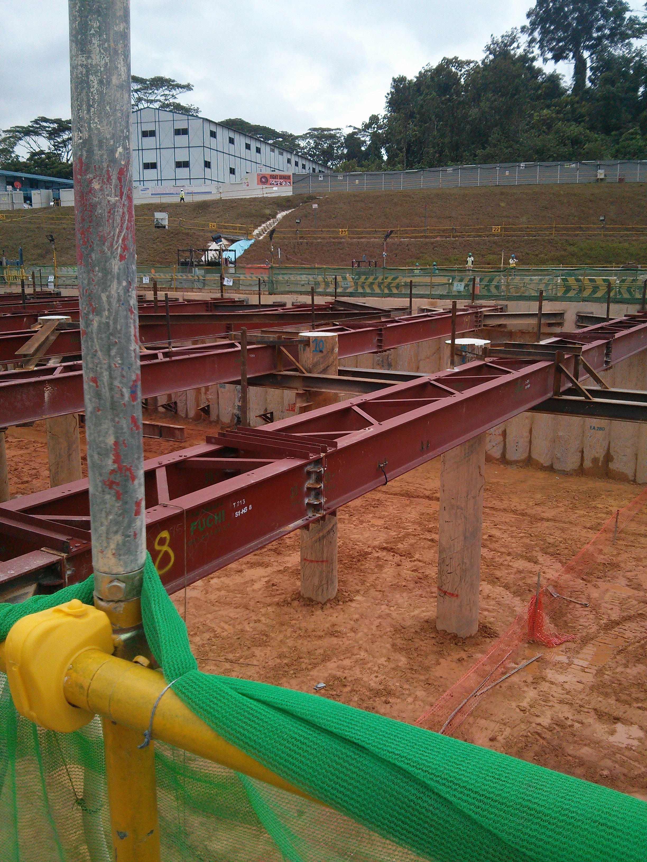
Figure 6: Excavation pit being prepared for the insertion of Level 2 struts.

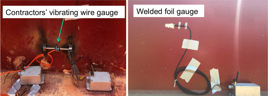
Figure 7: Example deployment on a strut next to vibrating wire gauges

The ReStructure nodes were mounted on to struts after it had been placed in the excavation, but before it had been pre–loaded: installation of the strut is completed by jacking preload forces into the strut to ensure that it remains in compression during subsequent excavation events. This allowed us to calibrate the WBF strain gauge in an unstressed/zero strain configuration. The WBF strain gauges were spot welded aligned to the length of the strut on the web (vertical section of strut, see Figure 7) and the strain bridge was manually balanced by adjusting the on-board potentiometer while the node is connected to a laptop displaying the current reading. This balancing procedure allows a reference point to be set that corresponds to zero load on the strut.

Figure 8 shows a schematic elevation of the cross section of the struts and the relative distance between the nodes and the gateway. Data was collected at 5 minute intervals, and nodes communicated on 802.15.4 channel 26 in an attempt to avoid any WI-FI interference and the maximum number of retries for each packet (sent by Contiki Collect) was set at 16.

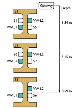
Figure 8: Deployment layout of ReStructure wireless bonded foil (WBF) strain gauges (50–56) and commercial vibrating wire (VW) gauges (VW-L1/L2) across three strut levels (S1, S2, S3). Distance from deployment location to gateway is shown in metres.

4.1 Network and energy performance

Table 4 shows the deployment duration and data yield across the deployment. There were two major outages where the node gateway batteries had exhausted: the first outage lasted 2.5 days (22nd to 24th June 2015) and the second outage lasted 19.3 days (10th to 29th September 2015), due to difficulties accessing the site. The data yield (or PDR) when ignoring the gateway outages is shown in the far right colum in Table 4.

Based on the analysis in Section 3.3, it was predicted that each node would have a best–case lifetime on 205 days. We see that both nodes on S2 got to within 10% of this prediction, where as the batteries in nodes on S1 and S3 lasted <50% less than expected. There are two potential explanations for this discrepancy - firstly, the effect of radio retransmissions and packet forwarding on lifetime (not analysed in this work), and secondly choice of battery. Nodes 50 and 52 were fitted with Energizer MAX Alkaline C cells, while the other nodes were fitted with Duracell PROCELL Alkaline C cells, suggesting that the Energizer batteries performed better for the energy consumption profile outlined in Section 3.3.

Table 4: Deployment summary for H14

Strut	Node	Deployed	Offline	Duration	Data	Data yield
level	ID			(days)	yield (%)	w/o
						outages (%)
S1	55	4th May	16th Aug	104	86.1%	88.2%
S1	51	4th May	26th Jul	82	91.1%	93.9%
S2	52	9th Jun	15th Dec	189	87.6%	99.0%
S2	50	9th Jun	11th Dec	185	87.4%	99.1%
S3	56	18th Jul	4th Nov	109	81.3%	98.7%

The Network configuration for the period 9th June to 4th November 2015, where all nodes were deployed and operating concurrently, is shown in Table 5. The network performance is evaluated using link stability, as defined in Section 3.4, as well as most common parent (MCP). The network was stable throughout ($>90$% stability for each node), and most often at S1 and S2, nodes chose to send directly to the sink. At S3, node 56 chose to send via S2 most often.

Table 5: Network configuration from 9th June 2015 to 4th November 2015 (148 days)

Strut	Node	Dist. to	Most common	MCP %	Stability
level	ID	sink (m)	parent
S1	55	1.34	Sink	98.4%	97.2%
S1	51	1.34	Sink	73.3%	92.7%
S2	52	5.15	Sink	86.7%	95.6%
S2	50	5.15	Sink	81.0%	93.9%
S3	56	8.59	50	64.6%	90.0%

Figure 9 shows an annotated graph of the daily PDR. In some cases, packet loss is specific to the node and is probably due to localised wireless interference or shadowing. Most loss, however, is concurrent indicating that the cause is most likely at the gateway.

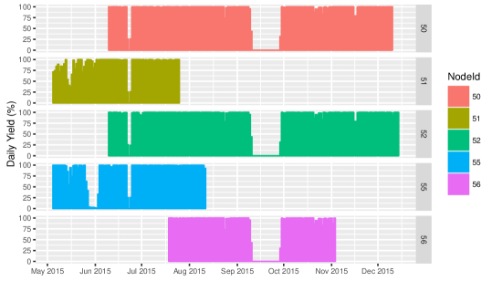
Figure 9: Daily PDR for Deployment 2 showing some independent yield loss (e.g., late May for node 55) and some concurrent loss (e.g., September for nodes 50, 52, 56). Concurrent losses are most likely due to gateway failure.

4.2 Strain measurement results

WBF strain data was collected by the ReStructure nodes at 5 minute intervals and VW strain data was collected by contractors at roughly hourly intervals.

• Figure 10 compares the VW strain measurements with the WBF strain gauge.

• The VW measurements are compensated for temperature and hence, aim to measure only the loads from the earth pressures.

• The VW data contain significant noise, skewed in the negative direction, possibly associated with electromagnetic interference and which is reduced in the figure by using a median filter ($k=5$).

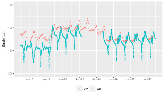
Figure 10: Comparison of vibrating wire (VW) and wireless bonded foil (WBF) strain measurements at S1-L1

• The WBF measurements could not be compensated using a factory polynomial as none was provided by the manufacturer. Therefore, we used part of the data to compensate under the assumption that temperature is the main cause of diurnal variation.

• To derive a thermal compensation curve for the WBF measurements, we used a LOESS fit to establish the overall trend for strain where the temperature was $27\pm 0.1\,\,\textrm{\textcelsius}$ and then found the residual strain (for all temperatures) against this fit.

  • This residual is then mapped to temperature as shown in Figure 11 to derive a temperature compensation curve.

  • Note that the effect on residual strain is larger (more negative) for the same temperature when the temperature is increasing (during the morning) than when the temperature is decreasing (during the evening).

  • Compensating for temperature does not completely remove the diurnal variation and there may be other factors (e.g., temperature at other locations, rate of change of temperature, or the time of day) that explain this variation.

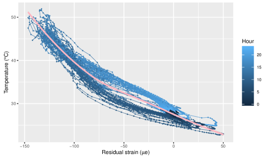
Figure 11: Residual strain versus temperature providing thermal compensation curve for S1-L1 node 51 along with a LOESS fit that was used to derive the compensated measurement shown in Figure 10.

• To allow comparison of the VW and WBF in terms of long-term trend, we examined the daily median strain over time, as shown in Figure 12.

• As shown in Table 6, most WBF sensors, with the exception of S1-L2 (Node 55), correlated well with the VW sensor at the same site.

• Although it is not clear what the cause of failure was, node 55 may have been affected by poor bonding of the foil to the strut.

• In the other WBF sensors, there is no drift in readings apparent.

• Correlated WBF sensors are offset from the corresponding VW sensors and this offset is probably due to differences in calibration procedures between the two. WBF sensors were zeroed prior to preloading whereas VW sensors were zeroed during preloading.

• Between stages, it is clear that the preloading phases for S2 and S3 had an effect on the strain measurement for the struts above them.

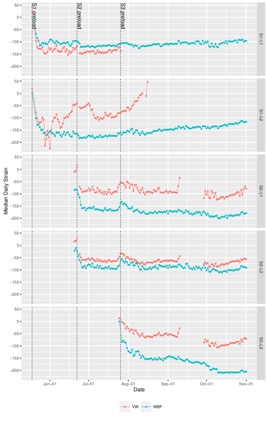
Figure 12: Daily median strain comparing WBF with VW

Table 6: Pearson correlation and mean difference (offset) for daily median strain of VW versus WBF over different sites

Site	Node	Correlation	Offset $\,\mathrm{\mu{}e}$
S1-L1	51	0.89	-26 $\pm$ 3
S1-L2	55	0.19	81 $\pm$ 10
S2-L1	50	0.83	83 $\pm$ 2
S2-L2	52	0.91	26 $\pm$ 1
S3-L2	56	0.93	98 $\pm$ 4

The contractor VW strain gauges are ’zeroed’ at the time when the pre-load is applied to the strut. Our WBF gauges were ’zeroed’ at some time prior to the preload, and we were not able to join during the process. This means there is an offset between our WBF measurements and the contractor VW measurements that is a function of the time of day they were zeroed, in terms of apparent strain and thermal loading. This offset problem is observable in all data, but particularly in Figure 13, which includes data from the load cell used to measure preloading through the jacking system.

Figure 13 shows the strain measurements converted into load (based on strut dimensions and the elastic modulus) and compared with the output of a load cell deployed on the strut and the VW estimated load. The load cell clearly shows a diurnal pattern that is in sync with the WBF strain measurements. These patterns are most likely an effect of temperature variation. The VW measurements show little or no variation with temperature, and have probably been adjusted to compensate for temperature.

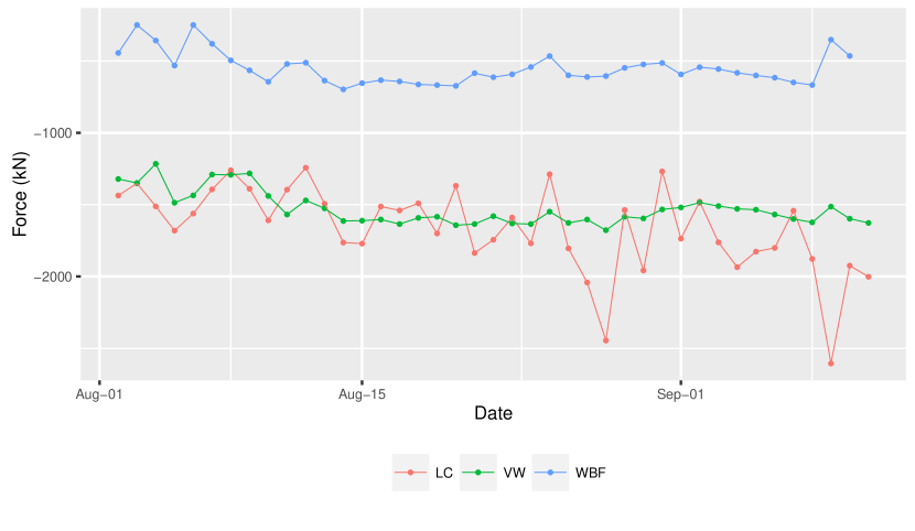
Figure 13: ReStructure strain gauge matches load cell; however both appear to be affected by temperature.

5 Lessons from the deployments and open challenges

The ReStructure deployments and the subsequent data analysis revealed a number of open questions for the WSN community as well as providing several insights into more practical aspects of the implementation and deployment that can increase the success of future projects if catered for.

5.1 Practical insights

Sensor node calibration

The current sensor node requires manual calibration on site, where environmental conditions can be extreme. Setting up and calibrating nodes in situ also requires a wired connection to the node. A wireless auto-calibration procedure (prompted remotely by the deployer of the network) for nodes once they have been installed could make the process faster and easier; alternatively, the balancing process could be ignored and offsets applied during data processing.

Sensor node communication

The current sensor network communication technology uses 802.15.4 compatible radios transmitting at $2.4\,\mathrm{GHz}$. It is possible that using a sub-1GHz frequency would increase the range and stability of the multi-hop low power network. A platform such as the Zolertia Remote  provides both $2.4\,\mathrm{GHz}$ and sub-$1\,\mathrm{GHz}$ radios, which could enable side-by-side tests. Unfortunately, in the current deployment we have been unable to perform a thorough analysis of the network operations for dual-band radios. ReStructure performed well when deployed over three strut levels, however the distance is only tens of metres. Intuitively, short transmission distance is not an issue in a sufficiently dense network (e.g., two nodes per strut). However, we did not deploy enough sensors to see how the network scales.

Sensor node packaging

The current sensor node is rated to IP65. We had however encountered instances of water ingress and one node had water damage during severe rainstorms. Improving the IP rating to IP67 or IP68 will ensure robustness.

Gateway

The current gateway design makes use of batteries that must be replaced every 30 days. A better design would be to add a solar panel to extend battery life. In addition, the addition of a sensor to measure and transmit battery charge level would have allowed better scheduling of maintenance visits.

5.2 Open design challenges

1. More reliable, lower maintenance networks would be necessary to meet performance requirements for accurate on line modelling and prediction of load in TERS; methods for identifying the optimal sampling rate, data transmission frequency and assessing connectivity changes can help meet this aim (possibly thorough analysis of network activity on various sites and evaluating the effects of evolving excavations). Observations of network behaviour at scale is also necessary to inform future developments. Open questions are to do with 1) the number of gateways needed for best performance, 2) adding in redundancy, 3) controlling the nodes and 4) implementing more dynamic operation of the network at run-time so that data may be acquired at higher rates when events of interest occur, such as strut pre-loading or excavation. This is important since the loading is expected to be static most of the time (excepting cyclic temperature variations that cause thermal loading).

2. Lower energy networks are needed to meet the longevity requirements—the ReStructure energy benchmarking section showed that 38% of a nodes energy requirement is for sensing, and 61% is for Contiki Collect operation (i.e. sending/forwarding packets and media access). To reduce the energy requirement of a node we would need to i) user lower power circuitry for the strain gauge signal conditioning hardware, and ii) use a (potentially) lower power network protocol, such as TDMA (Time division multiple access), would reduce the energy cost associated with listening.

3. Methods for detecting and compensating for thermal loading are needed in order to make strain gauges a viable solution for cheap and dense strain measurement.

6 Literature review

A number of works in the literature have inspired and guided this project, as well as providing baseline expectations for the deployments. Specifically, we looked at related applications of WSNs (platforms, packaging, and radio connectivity) for monitoring structural health.

Past research into monitoring of civil structures has attempted to: integrate experimental and numerical modelling of seismic damage in a three storey building (lab scale model) [9]; track performance of excavations during construction [17]; devise new sensing modalities applicable to structural health monitoring [1]; and assess the potential WSNs have for this field [8, 21]. While several recent works discuss aspects of WSN design for structural monitoring [5, 14, 23], there have been few long-term (i.e., running over several years) research projects related to the development and deployment of low-power wireless sensor network systems on bridges and tunnels. Table 7 shows a breakdown of notable projects surveyed, including one recent, but less developed work.

Table 7: Projects surveyed

Institution/Department	Project	Duration
The University of Illinois at Urbana Champaign (UIUC)	Illinois Structural Health Monitoring Project (ISHMP)	2002–
The University of Michigan (U of M)	Yeondae Bridge, Grove Street Bridge, Guendam Bridge	2004/5
The University of California Berkeley (UCB)	Structural Health Monitoring of the Golden Gate Bridge	2004–2006
Cambridge University and Imperial College London	Smart Infrastructure: Monitoring and Assessment of Civil Engineering Infrastructure	2006–2009
Swiss Federal Laboratories for Materials Testing and Research	Railway bridge monitoring	2014–

• In 2004/5, Lynch et al. [16] performed two deployments (2 days each) of a network of 14 custom sensor nodes (distance between nodes of $5.75$–$19\,\mathrm{m}$, over $46\,\mathrm{m}$), measuring acceleration/vibration for a concrete box girder bridge in Guemdang, Korea.

• In 2006, a UCB team carried out a deployment of a 64-node multi-hop network of MicaZ nodes ($2.4\,\mathrm{GHz}$) on the Golden Gate Bridge, sampling vibration/acceleration at $1\,\mathrm{kHz}$ (July 2006 to October 2006, with batteries changed in September 2006) [12]. Nodes were spaced $46\,\mathrm{m}$ apart (close to the limit of communication). The authors report average radio reception ranges around $30\,\mathrm{m}$ with a bi-directional antenna, decreasing to around $15\,\mathrm{m}$ in the presence of obstructions. The work informed our design choices particularly as the nodes placement was similar and provided expectation for transmission ranges in the excavation environment.

• As part of the EPSRC WINES project, Cambridge University has had several successful Structural Health Monitoring (SHM) deployments, including a 12-node WSN installed on the Humber Bridge (approx. $60\,\mathrm{m}$ distance from sink to furthest node), a 7-Node deployment on a concrete road bridge (approx. $30\,\mathrm{m}$) and a 26-node node deployment on the Jubilee line on the London Underground (approx. $180\,\mathrm{m}$ coverage). A key finding is the need for connectivity testing prior to deployment and further routing algorithms design that ensure fast convergence to speed up deployment [20].

• As part of the Illinois Structural Health Monitoring Project [19], the Jindo Bridge in South Korea has had extended deployment of sensors—70 in 2009, increased to 113 in 2011. Wind speed, acceleration and strain, were measured across a heterogeneous network. Multiple aspects of this deployment have been documented: Jang et al. [10] describe the hardware and physical deployment including details of the 4 networks (3 single hop networks of 23 nodes covering $175\,\mathrm{m}$, and 1 multi-hop network) and emphasise that antenna placement is key to increased transmission ranges, while Nagayama et al. [18] evaluated the use of multi-channel transmission to increase the available throughput of the network in high data rate applications.

• In 2014, Feltrin et al. [4] developed and deployed a custom sensor node for railway bridges to predict fatigue from train traffic. Their custom sensor node was based on the TI MSP430 SoC, and a sub-GHz radio. The deployment consisted of 7 nodes deployed for 13 days on a railway bridge in November 2014. Over the 13 days they achieved a PDR > 90% through an event-based system design. Similar to the ReStructure nodes, Feltrin et al. [3] note the large power requirement for sensing. They solve this issue by using low power components for their strain gauge signal conditioning hardware.

A variety of platforms were used in these projects. Commonly, wireless sensor nodes were constructed as a combination of i) an off-the-shelf radio / microprocessor platform and ii) a custom I/O board to provide the relevant functionality for the motivating application. We also follow this approach in this work. Software modules and operating systems are readily available for existing sensor node platforms (e.g., TinyOS and Contiki), however these platforms rarely provide the specialised on-board signal processing chains that are required for vibration, strain or other structural measurements. From deployments listed, only Lynch [13] developed a custom hardware platform, which is called the Narada.

Radios transmitting on the $2.4\,\mathrm{GHz}$ ISM band (TelosB, MicaZ and Imote) appear to be most common for structural monitoring projects, with the exception of Hao et al. [7] who also used Mica2 ($433\,\mathrm{MHz}$), and Lynch et al. [13] where a custom node with a $900\,\mathrm{MHz}$ radio was used. The platform of direct relevance here is the Imote2 based SHM platform [19]. This is a stackable board configuration that modularises the sensor node, data acquisition and signal conditioning to service a variety of applications. The SHM-S board is used to measure strain, and has undergone several stages of development to refine the circuitry and operation. It features built-in resistors to perform shunt calibration (i.e. fake strain values to test input/output range of the acquisition system) and a digitally controlled potentiometer to enable auto-balancing of a strain gauge in response to a system command. This type of functionality is desirable for a well-tested board that has undergone significant development but is over-complicated for a prototype strain circuit.

Radio connectivity and packaging impact the success of all practical deployments and are thus discussed in more detail below.

• In controlled experimentation with the Imote / CC2420 radio Rice [15] demonstrated that the use of an external, omnidirectional antenna (the Antenova Titanis) had a significant effect in terms of Received Signal Strength in an anechoic chamber when compared to an integrated/on board antenna. Subsequent field tests examining line of sight transmission ranges demonstrated that this antenna was capable of transmitting around 3 times the distance of the on-board chip antenna ($300\,\mathrm{m}$ compared to $100\,\mathrm{m}$). The authors also found the effect of transmitting through a steel / concrete floor (between floors in a University building at a distance of $6\,\mathrm{m}$) produced only a 10% reduction in reception rate when using the external antenna, compared to line of sight transmission between floors. Due to the improvement in reception rate using the external antenna, the same antenna has been integrated to the ReStructure node. However, we did not perform any comparison tests to assess performance.

• An investigation in 2010 [11] used 20 Narada nodes in an open parking lot to investigate the benefit of i) a custom amplifier on the standard $2.4\,\mathrm{GHz}$ radio ($10\,\mathrm{dB}$ amplification) and ii) directional antennas. With a standard antenna, maximum distance achievable is between $200\,\mathrm{m}$ (no amplification) and $300\,\mathrm{m}$ (amplification). With the directional antenna, the maximum distance increases to $500\,\mathrm{m}$ (no amplification) and $600\,\mathrm{m}$ (amplification). The power amplification has a significant cost to the sensor node power budget and so represents a design decision for specific applications, as does the directional antenna, which limits the configuration of the sensor network. Since, micro-benchmarking showed that the nodes would not meet the one year lifetime requirement, and we could not access the nodes post-deployment, the ReStructure node does not include a signal amplifier. Further as the deployment site was ever evolving we settled for an omni-directional antenna.

• In 2008, Hao et al. [7] performed a study of radio connectivity during the construction of Pasir Panjang MRT station in Singapore, as part of a project related to an Integrated Dual Radio Framework for sensor networks. This unpublished work examined the difference in radio connectivity between MicaZ ($2.4\,\mathrm{GHz}$) and Mica2 ($900\,\mathrm{MHz}$) sensor nodes. Unfortunately, the authors only deployed sensors at one side of the excavation, and then only at the top. The nodes performed a simple packet counting exercise, with individual nodes transmitting a burst of packets every 11 minutes while its neighbours counted the number of packets received. The longest period tested was for 5.5 days. The authors found positioning of the antenna is vital for connectivity. When the nodes were simply placed on the struts, the $2.4\,\mathrm{GHz}$ radio had slightly better performance (this result was duplicated in the lab with the nodes placed on the floor). However, when the antenna was raised, the opposite was true. In Feltrin’s [4] project they used a sub-GHz radio in their custom sensor to achieve better signal propagation as no nodes had line of sight. The ReStructure nodes used a $2.4\,\mathrm{GHz}$, however during range tests we discovered that communication range was a limiting factor. In future work, we aim to compare $2.4\,\mathrm{GHz}$ and sub-GHz radios. The choice of the radio frequency will affect the resulting network infrastructure. For example, longer transmission ranges may reduce the number of gateways required.

• A variety of different approaches have been used to attach sensors onto the structure being monitored. In one bridge monitoring project, enclosures and antennas were attached with G-clamps [12]. In the Jindo bridge project [19], magnets were used to connect the sensor nodes to the underside of the bridge along with curved brackets where nodes needed to be attached to support poles. In both projects, plastic enclosures were used.

7 Conclusions

The paper demonstrates that WSN based systems can be effectively used for monitoring load in TERS during excavation and construction processes. Through the design, implementation and deployments reported, we showed that, when well specified at design stage, WSNs:

• can operate, as required, in the field, unattended, and deliver data to a remote user application;

• can achieve consistently high data yield (observed between 81.3% to 91.1% in normal operating conditions) on single and multi-hop configurations, using $2.4\,\mathrm{GHz}$ radio, on active and dynamic construction sites, under extreme climatic conditions and in face of obstructions and interference common to excavation sites. Human error caused the greatest proportion of data loss;

• can evolve their network structure as the number of nodes increases while construction proceeds and depth of excavation increases;

• can be designed to function, on $2\times 7800\,\mathrm{mAh}$ C cells, for a duration of 6 months in sense-and-send mode, with 5 minute sampling interval.

Further research is however needed in order for such systems to achieve their full, large scale industrial potential:

• Solutions must be found to better compensate for apparent strain in the measurement system without removing the effects of thermal loading; ideally this would be done through in-field calibration under no-load conditions (before pre-loading), or using manufacturer provided polynomial coefficients based on batch testing during production;

• to enable future systems to minimise their power consumption and extend battery life, they will need network protocol and hardware optimisation as well as strategies for adaptive sampling;

• future systems must be easily deployable and self-calibrating to minimise deployment time in extreme deployment environments;

• understanding the impact on wireless communication and data collection capability of a full-scale deployment on a TERS, grown throughout the entirety of its life-cycle (a year or more);

• real-time integration of strain data with structural soil models also remains an open are of research that is worthy of consideration by the community–deriving tight requirements for the WSN from the model side and piloting full end-to-end systems is key to ensure full benefit is obtained from the WSN technologies

Increasing the density, timeliness and frequency of relatively cheap strain measurements on TERS can give new insight into the design and construction process. We can foresee smart struts where instrumentation is embedded into the support. At this stage the challenges lie in mass collection and integration of these measurements to motivate such a move to intelligent construction infrastructure.

References

- [1] Venu Gopal Madhav Annamdas and Yaowen Yang. Practical implementation of piezo-impedance sensors in monitoring of excavation support structures. Structural Control and Health Monitoring, 19(2):231–245, 2012.
- [2] J. Brusey, J. Kemp, E. Gaura, R. Wilkins, and M. Allen. Energy profiling in practical sensor networks: Identifying hidden consumers. IEEE Sensors Journal, PP(99), 2016.
- [3] Glauco Feltrin and Nemanja Popovic. Monitoring of strain cycles on a railway bridge with a wireless sensor network. IABSE Symposium Report, 105(21):1–8, 2015-09-23T00:00:00.
- [4] Glauco Feltrin, Nemanja Popovic, Kallirroi Flouri, and Piotr Pietrzak. A wireless sensor network with enhanced power efficiency and embedded strain cycle identification for fatigue monitoring of railway bridges. Journal of Sensors, 2016.
- [5] J.H. Galbreath, C.P. Townsend, S.W. Mundell, M.J. Hamel, B. Esser, D. Huston, and S.W. Arms. Civil structure strain monitoring with power-efficient, high-speed wireless sensor networks. In proceedings 4th International Workshop on Structural Health Monitoring, 2003.
- [6] Omprakash Gnawali, Rodrigo Fonseca, Kyle Jamieson, David Moss, and Philip Levis. Collection tree protocol. In Proceedings of the 7th ACM Conference on Embedded Networked Sensor Systems, SenSys ’09, pages 1–14, New York, NY, USA, 2009. ACM.
- [7] Shuai Hao, Mun Choon Chan, Bhojan Anand, and A L Ananda. Structure health monitoring at mrt construction sites using wireless sensor networks link measurement at pasir panjang station. Technical report.
- [8] T. Harms, S. Sedigh, and F. Bastianini. Structural health monitoring of bridges using wireless sensor networks. IEEE Instrumentation Measurement Magazine, 13(6):14–18, December 2010.
- [9] D. Isidori, E. Concettoni, C. Cristalli, L. Soria, and S. Lenci. Proof of concept of the structural health monitoring of framed structures by a novel combined experimental and theoretical approach. Structural Control and Health Monitoring, 23(5):802–824, 2016.
- [10] S. Jang, H. Jo, S. Cho, K. Mechitov, J. A. Rice, S. Sim, H. Jung, C-B Yun, B. F. Spencer Jr, and Gul A. Structural health monitoring of a cable-stayed bridge using smart sensor technology: deployment and evaluation. Smart Structures and Systems, 6(5-6):439–459, 2010.
- [11] Junhee Kim, Andrew Swartz, Jerome P Lynch, Jong-Jae Lee, and Chang-Geun Lee. Rapid-to-deploy reconfigurable wireless structural monitoring systems using extended-range wireless sensors. Smart Structures and Systems, 6(5-6):505–524, 2010.
- [12] S. Kim, S. Pakzad, D. Culler, J. Demmel, G. Fenves, S. Glaser, and M. Turon. Health monitoring of civil infrastructures using wireless sensor networks. In 2007 6th International Symposium on Information Processing in Sensor Networks, pages 254–263.
- [13] M. Kurata, J. Kim, J. P. Lynch, G. W. van der Linden, H. Sedarat, E. Thometz, P. Hipley, and L.-H. Sheng. Internet-enabled wireless structural monitoring systems: Development and permanent deployment at the new carquinez suspension bridge. Journal of Structural Engineering, 139(10):1688–1702, 2013.
- [14] Jian Li, Kirill A. Mechitov, Robin E. Kim, and Billie F. Spencer. Efficient time synchronization for structural health monitoring using wireless smart sensor networks. Structural Control and Health Monitoring, 23(3):470–486, 2016.
- [15] Lauren E. Linderman, J. A. Rice, Suhail Barot, B. F. Spencer Jr., and J. T. Bernhard. Characterization of wireless smart sensor performance. Journal of Engineering Mechanics, 136(12):1435–1443, 2010.
- [16] Jerome P Lynch, Yang Wang, Kenneth J Loh, Jin-Hak Yi, and Chung-Bang Yun. Performance monitoring of the geumdang bridge using a dense network of high-resolution wireless sensors. Smart Materials and Structures, 15(6):1561–1575, December 2006.
- [17] S. McLandrich, Y. Hashash, and N. O’Riordan. Networked geotechnical near real-time monitoring for large urban excavation using multiple wireless sensors. International Conference on Case Histories in Geotechnical Engineering, 2013.
- [18] Tomonori Nagayama, Parya Moinzadeh, Kirill Mechitov, Mitsushi Ushita, Noritoshi Makihata, Masataka Leiri, Gul Agha, Billie F Spencer Jr, Yozo Fujino, and Ju-Won Seo. Reliable multi-hop communication for structural health monitoring. Smart Structures and Systems, 6(5-6):481–504, 2010.
- [19] Jennifer A Rice, Kirill Mechitov, Sung-Han Sim, Tomonori Nagayama, Shinae Jang, Robin Kim, Billie F Spencer Jr, Gul Agha, and Yozo Fujino. Flexible smart sensor framework for autonomous structural health monitoring. Smart structures and Systems, 6(5-6):423–438, 2010.
- [20] Frank Stajano, Neil Hoult, Ian Wassell, Peter Bennett, and Civil Engineering. Smart bridges, smart tunnels: Transforming wireless sensor networks from research prototypes into robust engineering infrastructure. 0100, 2009.
- [21] Zhuoxiong Sun, Bo Li, Shirley J. Dyke, Chenyang Lu, and Lauren Linderman. Benchmark problem in active structural control with wireless sensor network. Structural Control and Health Monitoring, 23(1):20–34, 2016.
- [22] Wikipedia. Hostap — wikipedia, the free encyclopedia, 2012. [Online; accessed 8-July-2016].
- [23] Guang-Dong Zhou, Ting-Hua Yi, Huan Zhang, and Hong-Nan Li. Energy-aware wireless sensor placement in structural health monitoring using hybrid discrete firefly algorithm. Structural Control and Health Monitoring, 22(4):648–666, 2015.