Chiral Battery, scaling laws and magnetic fields

Abstract

We study the generation and evolution of magnetic field in the presence of chiral imbalance and gravitational anomaly which gives an additional contribution to the vortical current. The contribution due to gravitational anomaly is proportional to $T^{2}$ which can generate seed magnetic field irrespective of plasma being chirally charged or neutral. We estimate the order of magnitude of the magnetic field to be $10^{30}$ G at $T\sim 10^{9}$ GeV, with a typical length scale of the order of $10^{-18}$ cm, which is much smaller than the Hubble radius at that temperature ($10^{-8}$ cm). Moreover, such a system possess scaling symmetry. We show that the $T^{2}$ term in the vorticity current along with scaling symmetry leads to more power transfer from lower to higher length scale as compared to only chiral anomaly without scaling symmetry.

1 Introduction

In the standard model of cosmology, it is usually assumed that the early Universe is composed of plasma of elementary particles and the long range fields are absent. However the observed magnetic field, which requires initial seed and its subsequent amplification, is one exception. Moreover, the existence of large scale magnetic field indicates toward its primordial origin. Till date, various mechanism have been proposed to generate such magnetic field [1, 2, 3, 4, 5, 6, 7, 8, 9, 10, 11, 12, 13, 14, 15, 16].

Recently, considerable attention is being paid to investigate the role of quantum chiral anomaly in the generation of primordial magnetic field. It was argued that processes in the early Universe, at temperature much above electroweak scale ($T\sim 100$GeV), can lead to more number of right-handed particles than left-handed ones and they remain in thermal equilibrium via its coupling with the hypercharge gauge bosons [17, 18]. Their number is effectively conserved at those scales which allow us to introduce the chiral chemical potentials. Furthermore, in presence of either external gauge field or rotational flow of the fluid, there could be a current in the direction parallel to the external field or parallel to the vorticity generated due to rotational flow of the chiral plasma. The current along the external magnetic field in presence of chiral imbalance is known as the “chiral magnetic current” and the phenomenon is called the “Chiral Magnetic Effect” (CME) [19, 20, 21, 22, 23]. Similarly, the current parallel to the rotation axis is known as “chiral vortical current” and the phenomenon is called “Chiral Vortical Effect” (CVE) [24, 25, 26, 27, 28]. CME and CVE are characterized by the respective coefficients $\xi^{(B)}$ and $\xi$.

In the presence of quantum anomalies for global current there exist a term $\xi\,\omega^{\mu}$, with $\omega^{\mu}\sim\epsilon^{\mu\nu\lambda\rho}\,u_{\nu}\partial_{\lambda}u_{\rho}$, in the conserved current [27]. It has been argued that the vorticity induced current $\xi\,\omega^{\mu}$ is not only allowed, but is required by anomalies [27]. By demanding that the derivative of the entropy current $s^{\mu}$ is non-negative i.e. $\partial_{\mu}\,s^{\mu}\geqslant 0$, the coefficient $\xi$ can be expressed in terms of chemical potential, number density, energy density $\rho$ and pressure density $p$. In [29] authors have studied the generation and evolution of magnetic field in presence of vortical current due to chiral imbalance. However, if we have $n_{L}+n_{R}=0$ which imples $\mu=\mu_{L}+\mu_{R}=0$, then the chiral vortical coefficient $\xi\sim(\mu_{R}^{2}-\mu_{L}^{2})/\sigma$ will vanish. As a consequence, there will not be any seed magnetic field as discussed in [29]. Interestingly, there are situations where vortical conductivity is proportional to $T^{2}$ [28, 21]. The origin of $T^{2}$ term in the vortical conductivity is attributed to the gravitational anomaly which arises when gauge fields are coupled to gravity (for detailed discussion on gravitational anomaly see [30]. A first principle calculation of transport coefficients using Kubo formula leads to anomalous vortical conductivity containing a term $\propto T^{2}~{}$ which may be due to $~{}C_{\rm g}~{}\epsilon^{\mu\nu\rho\lambda}~{}R^{\alpha}_{~{}~{}\beta\mu\nu}~{}R^{\beta}_{~{}~{}\alpha\rho\lambda}$, with $C_{\rm g}$ being the gravitational anomaly coefficient, in the expression for the anomaly equation [30, 28]. Although, the gravitational anomaly is fourth order in the metric derivatives though they contributes to first order in the transport coefficients. One plausible explanation is that the gravitational field in the presence of matter gives rise to a fluid velocity $u^{\mu}$ e.g. through frame dragging effects and might effectively reduce the number of derivatives that enter in the hydrodynamic expansion [28].

In the early Universe where chemical potential of the species is much smaller than the temperature, the dominant contribution to the vortical current comes from $T^{2}$. As a consequence, the seed magnetic field can be generated in the early Universe irrespective of fluid being chirally neutral or charged. On the other hand, the equations of chiral magnetohydrodynamics (ChMHD), in absence of other effects like charge separation effect and cross helicity, follow unique scaling property and transfer energy from small to large length scales.

In this work we will consider the correction to the current density due to gravitational anomaly and show that the seed magnetic field can be generated in the every early universe. We will solve the diffusivity equation in an expanding background. Rather than solving the Navier-Stroke’s equation for velocity spectrum, we will consider the scaling symmetries, consistent with $T^{2}$ term in the vorticity current, given in [31] to obtain the velocity spectrum. We show that the amount of energy at large length scale under scaling symmetry is more than previous study where only chiral anomaly was considered [29].
This paper is organized as follows: in section 2 we will provide the brief description of the chiral fluid and discuss the generation of seed magnetic field due $T^{2}$ term in the current density in section 3. We discuss about the scaling properties of the chiral plasma in section 3.2. We will provide the results in section 4 and Finally conclude in section 5

2 Overview of Chiral fluid

The dynamics of a plasma consisting of chiral particles in presence of background fields is governed by the following hydrodynamic equations

$$\nabla_{\mu}\,T^{\mu\nu}=F^{\nu\lambda}\,j_{\lambda}\,,$$ (2.1)

$$\nabla_{\mu}\,j_{\rm v}^{\mu}=0\,,$$ (2.2)

$$\nabla_{\mu}\,j_{5}^{\mu}=C\,E_{\mu}\,B^{\mu}\,,$$ (2.3)

where the vector current $j_{\rm v}^{\mu}=j^{\mu}_{R}+j^{\mu}_{L}$ and chiral current $j_{5}^{\mu}=j^{\mu}_{R}-j^{\mu}_{L}$ with $j_{R(L)}$ being the current density for right (left) handed particles. The chiral anomaly coefficient is denoted by $C$. In the state of local equilibrium, the energy momentum tensor $T^{\mu\nu}$, the vector current $j^{\mu}$ and the chiral current $j^{\mu}_{5}$ can be expressed in terms of the four velocity of the fluid $u^{\mu}$, energy density $\rho$, vector charge density $n_{\rm v}$ and axial charge density $n_{5}$ and these quantities respectively takes the following form

$$T^{\mu\nu}=(\rho+p)\,u^{\mu}\,u^{\nu}\,+p\,g^{\mu\nu}\,,$$ (2.4)

$$j^{\mu}_{\rm v}=n_{\rm v}\,u^{\mu}+\sigma E^{\mu}+\xi_{\rm v}\omega^{\mu}+\xi_{\rm v}^{(B)}B^{\mu}\,,$$ (2.5)

$$j_{5}^{\mu}=n_{5}\,u^{\mu}+\xi_{\rm 5}\omega^{\mu}+\xi_{5}^{(B)}B^{\mu}\,,$$ (2.6)

where $n_{\rm v,5}=n_{R}\pm n_{L}$, $\xi_{\rm v,5}=\xi_{R}\pm\xi_{L}$, $\xi^{(B)}_{\rm v,5}=\xi^{(B)}_{R}\pm\xi^{(B)}_{L}$, $\omega^{\mu}=\epsilon^{\mu\nu\sigma\delta}\,u_{\nu}\partial_{\sigma}\,u_{\delta}$ is the vorticity four vector, $E^{\mu}=F^{\mu\nu}\,u_{\nu}$, and $B^{\mu}=1/2\,\epsilon^{\mu\nu\sigma\delta}\,u_{\nu}\,F_{\sigma\delta}$. In presence of chiral imbalance and gravitational anomaly, consistency with second law of thermodynamics ($\partial_{\mu}\,s^{\mu}\geq 0$, with $s^{\mu}$ being the entropy density) demand that the coefficients, for each right and left particle, have the following form [27, 28, 21]

$$\xi_{i} = C\,\mu_{i}^{2}\,\left[1-\frac{2\,n_{i}\,\mu_{i}}{3\,(\rho+p)}\right]\,+\frac{D\,T^{2}}{2}\left[1-\frac{2\,n_{i}\,\mu_{i}}{(\rho+p)}\right]\,,$$ (2.7)

$$\xi_{i}^{(B)} = C\,\mu_{i}\,\left[1-\frac{n_{i}\,\mu_{i}}{2\,(\rho+p)}\right]\,-\frac{D}{2}\left[\frac{n_{i}\,T^{2}}{(\rho+p)}\right]\,.$$ (2.8)

The constants $C$ and $D$ are related to those of the chiral anomaly and mixed gauge-gravitational anomaly as $C=\pm 1/4\pi^{2}$ and $D=\pm 1/12$ for right and left handed chiral particles respectively. It is now easy to see from eq.(2.7) and eq.(2.8) that for $\mu_{i}/T\ll 1$, which is the scenario in the early universe, $\xi_{i}\sim\frac{D}{2}\,T^{2}$ and $\xi_{i}^{(B)}\sim C\,\mu_{i}$. Note that, $\xi_{\rm v}=0=\xi_{\rm v}^{(B)}$. However, $\xi_{5}\sim|D|T^{2}$ and $\xi_{5}^{(B)}=|C|\,(\mu_{R}-\mu_{L})=|C|\,\mu_{5}$. We would like to emphasize here that the $\xi_{5}$ is independent of chiral imbalance and depends only on the temperature. Thus, we expect such term to dominate at high temperature. We exploit this dominance to generate the magnetic field in the early Universe.

In an expanding background, the line element can be described by Friedmann-Robertson-Walker metric,

$$ds^{2}=a^{2}(\eta)\left(-d\eta^{2}+\delta_{ij}dx^{i}\,dx^{i}\right)\,,$$ (2.9)

where $a$ is the scale factor and $\eta$ is the conformal time. We choose $a(\eta)$ to have dimensions of length, and $\eta$ , $x^{i}$ to be dimensionless. Using the fact that the scale factor $a=1/T$, we can define the conformal time $\eta=M_{*}/T$, where $M_{*}=\sqrt{90/8\,\pi^{3}\,g_{\rm eff}}M_{P}$ with $g_{\rm eff}$ being the effective relativistic degrees of freedom that contributes to the energy density and $M_{P}=1/\sqrt{G}$ being the Planck mass. We also define the following comoving variables

$$\vec{B}_{c}=a^{2}(\eta)\,\vec{B}(\eta)\,,~{}~{}~{}\mu_{c}=a(\eta)\,\mu\,,~{}~{}~{}\sigma_{c}=a(\eta)\,\sigma\,,~{}~{}~{}T_{c}=a(\eta)\,T,~{}~{}~{}x_{c}=x/a(\eta)\,.$$ (2.10)

In terms of comoving variables, the evolution equations of fluid and electromagnetic fields are form invariant [32, 33, 34]. Thus, in the discussion below, we will work with the above defined comoving quantities and omit the subscript $c$.

Using the effective Lagrangian for the standard model, one can derive the generalized Maxwell’s equation [35],

$$\vec{\nabla}\times\vec{B}=\vec{j}\,,$$ (2.11)

with $\vec{j}=j_{\rm v}+j_{5}$ being the total current. In the above equation, we have ignored the displacement current. Taking $u^{\mu}=(1,\vec{v})$ and using eq.(2.5)- eq.(2.6), one can show that

$$j^{0} =n=n_{\rm v}+n_{5}\,$$ (2.12)

$$\vec{j} =n\vec{v}+\sigma(\vec{E}+\vec{v}\times\vec{B})+\xi\,\vec{\omega}+\xi^{(B)}\,\vec{B}\,,$$

with $\xi=\xi_{\rm v}+\xi_{5}$ and $\xi^{(B)}=\xi^{(B)}_{\rm v}+\xi^{(B)}_{5}$. For our analysis, we assume that the velocity field is divergence free, i.e. $\vec{\nabla}\cdot\vec{v}=0$. Taking curl of the eq.(2.11) and using the expression for current from eq.(2.12), we get

$$\frac{\partial\vec{B}}{\partial\eta}=\frac{n}{\sigma}\,\vec{\nabla}\times\vec{v}+\frac{1}{\sigma}\,\nabla^{2}\vec{B}+\vec{\nabla}\times(\vec{v}\times\vec{B})+\frac{\xi}{\sigma}\,\vec{\nabla}\times\vec{\omega}+\frac{\xi^{(B)}}{\sigma}\,\vec{\nabla}\times\vec{B}\,.$$ (2.13)

In obtaining the above equation, we have also assumed that chemical potential and the temperature are homogeneous. Note that, in the limit $\sigma\rightarrow\infty$, we will obtain magnetic fields which are flux frozen. There are other conditions in the cosmological and astrophysical settings in which the advection term $\vec{\nabla}\times(\vec{v}\times\vec{B})$ can be ignored compared to other terms and reduces the above equation to linear equation in $v$ and $B$. We ignore advection term in our analysis.

3 Chiral battery

In absence of any background magnetic fields $\vec{B}=0$, eq.(2.13) reduces to

$$\frac{\partial\vec{B}}{\partial\eta}=\frac{1}{\sigma}n\vec{\nabla}\times\vec{v}~{}+~{}\frac{1}{\sigma}\,\xi\,\vec{\nabla}\times\vec{\omega}\,.$$ (3.1)

Note that the two terms on the right hand side of eq.(3.1) no longer depends on $B$. This situation is similar to that of the Biermann battery mechanism where $\vec{\nabla}\rho\,\times\,\vec{\nabla}p$ term is independent of $B$ [36]. For Biermann mechanism to work, $\vec{\nabla}\rho$ and $\vec{\nabla}p$ have to be in different directions which can be achieved if the system has vorticity. In our scenario, it is interesting to note that even if $n=0$, $T^{2}$ term in $\xi$ will act as a source to generate the seed magnetic field at high temperature. On the other hand, in presence of finite chiral imbalance (such that $\mu/T\ll 1$) in the early universe, $T^{2}$ term in $\xi$ will still be the source to generate the seed magnetic field, but non-zero $\xi^{(B)}$ will lead to the instability in the system. An order of magnitude estimate gives the first term of eq.(3.1) to be $\frac{\alpha}{L}\,\left(\frac{\mu}{T}\right)\,T^{2}\,v$ while the second term is of the order $\frac{\alpha}{L^{2}}\,D\,T\,v$. On comparing the two terms we get a critical length $\lambda_{\rm c}\sim(D/T)(\mu/T)^{-1}$ below which first term will be sub-dominant.

3.1 Mode decomposition

In order to solve Eq.(3.1), we decompose the divergence free vector fields in the polarization modes, $\varepsilon^{\pm}_{i}$,

$$\boldsymbol{\varepsilon}^{\pm}({\boldsymbol{k}})=\frac{\boldsymbol{e}_{1}({\boldsymbol{k}})\,\pm\,i\boldsymbol{\,e}_{2}({\boldsymbol{k}})}{\sqrt{2}}\,\exp(i\,{\boldsymbol{k}}\cdot{\boldsymbol{x}})\,.$$ (3.2)

These modes are the divergence-free eigenfunctions of the Laplacian operator forming an orthonormal triad of unit vectors $(\boldsymbol{e}_{1},\boldsymbol{e}_{2},\boldsymbol{e}_{3}=\boldsymbol{k}/k)$. It is evident that $\nabla\cdot\boldsymbol{\varepsilon}^{\pm}=0$ and $\nabla\times\boldsymbol{\varepsilon}^{\pm}=\pm\,k\,\boldsymbol{\varepsilon}^{\pm}$. For our work $\boldsymbol{\varepsilon}^{\pm*}(-\boldsymbol{k})=\boldsymbol{\varepsilon}^{\pm}(\boldsymbol{k})$. We decompose the velocity of the incompressible fluid as:

$$\boldsymbol{v}(\eta,\boldsymbol{x})=\int\frac{d^{3}\,k}{(2\pi)^{3}}\,\left[\tilde{v}^{+}(\eta,\boldsymbol{k})\boldsymbol{\varepsilon}^{+}(\boldsymbol{k})+\tilde{v}^{-}(\eta,\boldsymbol{k})\boldsymbol{\varepsilon}^{-}(\boldsymbol{k})\right]\,$$ (3.3)

where, tilde denote the Fourier transform of the respective quantities. Assuming no fluid helicity and statistically isotropic correlators,

$$\langle\boldsymbol{\tilde{v}}^{\pm*}(\eta,\boldsymbol{k})\,\boldsymbol{\tilde{v}}^{\pm}(\eta,\boldsymbol{q})\rangle = (2\,\pi)^{3}\,\delta^{(3)}(\boldsymbol{k}-\boldsymbol{q})|\boldsymbol{v}(\eta,k)|^{2}$$ (3.4)

$$\langle\boldsymbol{\tilde{v}}^{+*}(\eta,\boldsymbol{k})\,\boldsymbol{\tilde{v}}^{-}(\eta,\boldsymbol{q})\rangle = \langle\boldsymbol{\tilde{v}}^{-*}(\eta,\boldsymbol{k})\,\boldsymbol{\tilde{v}}^{+}(\eta,\boldsymbol{q})\rangle=0\,,$$ (3.5)

the kinetic energy density can be given as

$$\frac{1}{2}\langle|\boldsymbol{v}(\eta,\boldsymbol{x})|^{2}\rangle=\frac{1}{2}\int d\log\,k\,E_{\boldsymbol{v}}(\eta,k)=\int\frac{d^{3}k}{(2\pi)^{3}}\left[|\boldsymbol{v}^{+}(\eta,\boldsymbol{k})|^{2}\,+\,|\boldsymbol{v}^{-}(\eta,\boldsymbol{k})|^{2}\right]\,.$$ (3.6)

Similar to the velocity field, we can decompose the magnetic field as,

$$\boldsymbol{B}(\eta,\boldsymbol{x})=\int\frac{d^{3}\,k}{(2\pi)^{3}}\,\left[\tilde{B}^{+}(\eta,\boldsymbol{k})\boldsymbol{\varepsilon}^{+}(\boldsymbol{k})+\tilde{B}^{-}(\eta,\boldsymbol{k})\boldsymbol{\varepsilon}^{-}(\boldsymbol{k})\right]\,.$$ (3.7)

The magnetic energy density is then given by

$$\frac{1}{2}\langle|\boldsymbol{B}(\eta,\boldsymbol{x})|^{2}\rangle=\frac{1}{2}\int d\log\,k\,E_{\boldsymbol{B}}(\eta,k)=\int\frac{d^{3}k}{(2\pi)^{3}}\left[|\boldsymbol{B}^{+}(\eta,\boldsymbol{k})|^{2}\,+\,|\boldsymbol{B}^{-}(\eta,\boldsymbol{k})|^{2}\right]\,.$$ (3.8)

Mode decomposition of Eq.(3.1) gives

$$\frac{\partial\tilde{B}^{+}}{\partial\eta} = \frac{1}{\sigma}\left(n\,k\,+\xi\,k^{2}\,\right)\tilde{v}^{+}\,,$$ (3.9)

$$\frac{\partial\tilde{B}^{-}}{\partial\eta} = \frac{1}{\sigma}\left(-n\,k\,+\xi\,k^{2}\,\right)\tilde{v}^{-}\,.$$ (3.10)

In absence of external fields, the energy momentum conservation equation $\nabla_{\mu}\,T^{\mu\nu}=0$ implies that $n$, $\sigma$ and $\xi$ are constant over time. Thus, the solution to Eq.(3.9) and Eq.(3.10) is

$$\tilde{B}^{\pm}(\eta,\boldsymbol{k})=\frac{1}{\sigma}\left(\pm n\,k\,+\xi\,k^{2}\,\right)\int_{\eta_{0}}^{\eta}\,d\eta^{\prime}\tilde{v}^{\pm}(\eta^{\prime},\boldsymbol{k})\,.$$ (3.11)

where $\eta_{0}=M_{*}/T_{0}$ and we have set $T_{0}=10^{10}$ GeV for our work. Multiplying Eq.(3.9) by $\tilde{B}^{+*}$ and Eq.(3.10) by $\tilde{B}^{-*}$, the ensemble average of the combined equation leads to

$$\frac{\partial|\tilde{B}^{+}|^{2}}{\partial\eta} = \frac{2}{\sigma}\left(n\,k\,+\xi\,k^{2}\,\right)\langle\tilde{B}^{+*}\tilde{v}^{+}\rangle$$ (3.12)

$$\frac{\partial|\tilde{B}^{-}|^{2}}{\partial\eta} = \frac{2}{\sigma}\left(-n\,k\,+\xi\,k^{2}\,\right)\langle\tilde{B}^{-*}\tilde{v}^{-}\rangle\,.$$ (3.13)

On using the solution obtained in Eq.(3.11) and the velocity decomposition given in Eq.(3.3) we obtain

$$\langle\tilde{B}^{\pm*}(\eta,\boldsymbol{k})~{}\tilde{v}^{\pm}(\eta,\boldsymbol{k}^{\prime})\rangle=\,\frac{1}{\sigma}\left(\pm n\,k\,+\xi\,k^{2}\,\right)\int_{\eta_{0}}^{\eta}d\eta^{\prime}\langle\tilde{v}^{\pm*}(\eta^{\prime},\boldsymbol{k})~{}~{}\tilde{v}^{\pm}(\eta,\boldsymbol{k}^{\prime})\rangle\,.$$ (3.14)

It is reasonable to expect that any $k$ mode of the fluid velocity to be correlated on the time scale $\tau\equiv|\eta-\eta^{\prime}|\sim 2\pi/k\,v$ and uncorrelated over longer time scales, where $v$ represents the average velocity of the fluid within the correlation scale. Thus, we can write

$$\langle\tilde{v}^{\pm*}(\eta^{\prime},\boldsymbol{k})~{}~{}\tilde{v}^{\pm}(\eta,\boldsymbol{k}^{\prime})\rangle=\left\{\begin{array}[]{ll}(2\pi)^{3}\langle v^{\pm}(\eta,\boldsymbol{k})^{2}\rangle\delta^{(3)}(\boldsymbol{k}-\boldsymbol{k^{\prime}})&\mbox{ for $\tau<\frac{2\pi}{k\,v}$}\\ \\ 0&\mbox{ for $\tau>\frac{2\pi}{k\,v}$ }\end{array}\right.$$ (3.15)

On using the above unequal time correlator in eq.(3.14), we obtain

$$\langle\tilde{B}^{\pm*}(\eta^{\prime},\boldsymbol{k})\tilde{v}^{\pm}(\eta,\boldsymbol{k}^{\prime})\rangle=\frac{(2\pi)^{3}}{\sigma}|v^{\pm}|^{2}\left(\pm nk+\xi\,k^{2}\right)~{}f(\eta,k)\delta^{(3)}(\boldsymbol{k}-\boldsymbol{k^{\prime}})$$ (3.16)

where $f(\eta,k)=\eta-\eta_{0}$ for $\eta-\eta_{0}\leq 2\pi/(k\,v)$ and zero otherwise.

3.2 Scaling properties in chiral plasma

It has been shown that ChMHD equations for electrically neutral plasma with chirality imbalance have scaling symmetry under following transformation [31],

$$\boldsymbol{x}\rightarrow\ell x\,,\hskip 14.22636pt\eta\rightarrow\ell^{1-h}\,\eta\,,\hskip 14.22636pt\boldsymbol{v}\rightarrow\ell^{h}\,\boldsymbol{v},$$

$$\boldsymbol{B}\rightarrow\ell^{h}\boldsymbol{B}\,,\hskip 14.22636pt\sigma\rightarrow\ell^{1+h}\,\sigma$$ (3.17)

with $\ell>0$ is the scaling factor and $h\in\Re$ is the parameter, under certain conditions [31]. With the above scaling, the fluid velocity spectrum is given by

$$E_{v}(\boldsymbol{k},\eta)\,k^{1+2\,h}=\psi_{v}(\boldsymbol{k},\eta)$$ (3.18)

where $\psi_{v}$ satisfies

$$\psi(k/\ell,\ell^{1-h}\,\eta)=\psi(k,\eta)\,.$$ (3.19)

On differentiating eq.(3.19) with respect to $\ell$ and taking $\ell=1$ leads to the following differential equation [37]

$$-k\frac{\partial\psi_{v}}{\partial k}+(1-h)\,\eta\,\frac{\partial\psi_{v}}{\partial\eta}=0\,,$$ (3.20)

which can be solved to obtain the form of $\psi$. The solution to the above differential equation can be given as

$$\psi_{v}(\eta,k)\propto\,k^{m}\,\eta^{m/(1-h)}\,,$$ (3.21)

where $m$ is a constants and taken as parameter in this work whose value is fixed by assuming Kolmogorov spectrum for $k>k_{i}$ and white noise spectrum for $k<k_{i}$, where $k_{i}$ is the wave number in the inertial range. From eq.(3.18) and eq.(3.21) , we get

$$E_{v}(\eta,k)=v_{i}^{2}\,\left(\frac{k}{k_{i}(\eta)}\right)^{-1-2h+m}\,\left(\frac{\eta}{\eta_{0}}\right)^{\frac{m}{1-h}}\,.$$ (3.22)

where $v_{i}$ is some arbitrary function which encodes the information about the boundary conditions. Therefore, the $k$ and $\eta$ dependence of fluid velocity can be given by

$$v(k,\eta)=v_{i}\,\left(\frac{k}{k_{i}(\eta)}\right)^{(-1-2h+m)/2}\,\left(\frac{\eta}{\eta_{0}}\right)^{\frac{m}{2(1-h)}}\,.$$ (3.23)

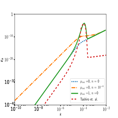
(a) Subfigure 1 list of figures text

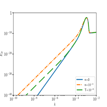
(b) Subfigure 2 list of figures text

Figure 1: Magnetic energy spectrum as a function of mode is shown: (a) when $n=0$, the $E_{B}$ goes as $~{}k^{7}$ at large length scale. However, the power is more than [29] at given $k$. (b) when $n\neq 0$, $E_{B}$ goes as $~{}k^{5}$ at large length scale. In both the figures we have set $T=10^{9}$ GeV and $v=10^{-4}$.

We are interested in an electrically neutral plasma with chiral charge. For such a system $h=-1$ [31]. However, in the radiation dominated epoch the fluid velocity does not change for $k<k_{i}(\eta)$. Assuming white noise on such scale, which implies $E_{v}\propto k^{3}$, we obtain

$$k_{i}(\eta)=k_{i}(\eta_{0})\,\left(\frac{\eta}{\eta_{0}}\right)^{1/3}$$ (3.24)

Substituting the value of $k_{i}(\eta)$ in eq.(3.23) we get

$$v(k,\eta)=v_{i}\,\left(\frac{k}{k_{i}(\eta_{0})}\right)^{(1+m)/2}\,\left(\frac{\eta}{\eta_{0}}\right)^{(m-2)/6}\,.$$ (3.25)

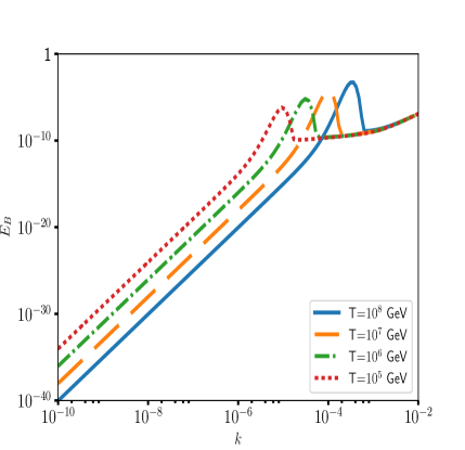
(a) Subfigure 1 list of figures text

(b) Subfigure 2 list of figures text

Figure 2: (a) Evolution of magnetic energy density $E_{B}$ as a function of $k$ and (b) Evolution of magnetic helicity density $\mathcal{H}_{B}$ as a function of $k$ for different temperature. As temperature ($T\sim 1/\eta$) decreases, peak shifted from higher to lower $k$ values which shows transfer of magnetic energy from small to large length scale. In both the figures we have set $v=10^{-4}$ and $n=10^{-4}.$

In absence of kinetic helicity in the fluid, eq.(3.6) implies $|v^{+}|=|v^{-}|=\pi k^{-3/2}\,v$.

3.3 Evolution of Magnetic field

Once seed field is generated it may start influencing the subsequent evolution of the system at certain mode. In that case, there will be a current flowing parallel to these generated magnetic fields. Therefore, we need to consider the effect of CME in the evolution Eq.(2.13). We can decompose this Eq.(2.13) in terms of polarization to obtain

$$\frac{\partial|\tilde{B}^{\pm}|^{2}}{\partial\eta}=\frac{2}{\sigma}\left(-k^{2}\pm\xi^{(B)}k\right)|\tilde{B}^{\pm}|^{2}+\frac{2}{\sigma^{2}}\left(\pm n\,k\,+\xi\,k^{2}\,\right)^{2}\,|v^{\pm}|^{2}\,f(\eta,k)$$ (3.26)

It is evident from the above equation that when the first term dominates over the second, then

$$|B^{\pm}|^{2}=|B_{0}^{\pm}|^{2}\exp\left(\frac{2\,\eta}{\sigma}\,k_{\rm ins}^{2}\right)\,\exp\left(\frac{2\,\eta}{\sigma}(k\mp k_{\rm ins})^{2}\right)$$ (3.27)

where $k_{\rm ins}=\xi^{(B)}/2$. From eq.(3.26), evolution of magnetic energy can be found as

$$\frac{\partial E_{B}}{\partial\eta}=\frac{-2\,k^{2}}{\sigma}E_{B}+\frac{2\,\xi^{(B)}\,k}{\sigma}\mathcal{H}_{B}+\frac{2}{\sigma^{2}}(n^{2}k^{2}+\xi^{2}k^{4})E_{v}f(\eta,k)$$ (3.28)

where $E_{B}$, $E_{v}$ and $\mathcal{H}_{B}$ are respectively magnetic energy, kinetic energy and magnetic helicity which effects the evolution of $\mu_{5}$ through the following equation

$$\frac{d\mu_{5}}{d\eta}=-2\alpha\int\frac{d\ln k}{k}\,\frac{\partial\mathcal{H}_{B}}{\partial\eta}\,-\Gamma_{f}\,\mu_{5}\,,$$ (3.29)

where $\Gamma_{f}$ is the chirality flipping rate. The flipping depends on interaction of the right handed particles with the Higgs and their back reaction [38]. At temperature $T\geq 80$ TeV the chirality flipping rate is much slower than the Hubble expansion rate. Therefore, eq.(3.29) can be rewritten as

$$\frac{\partial}{\partial\eta}\left[\mu_{5}+2\alpha\int\frac{d\ln k}{k}{\mathcal{H}}_{B}\right]=0\,.$$ (3.30)

The terms in the bracket is constant in time. Therefore, the helicity will be produced at the cost of chiral imbalance. However, when temperature drops to an extent that the flipping rate becomes comparable to the expansion rate of the Universe, maximally helical field will be generated. In order to get the complete picture of generation and evolution of the magnetic field, we solve eq.(3.26) along with eq.(3.29).

4 Results

In the early Universe, much before electroweak symmetry breaking, collision of bubble walls during first order phase transition at GUT scale, can generate initial vorticity in the plasma. With these assumptions, we have shown that magnetic field can be generated due to any of the two terms on the right hand side of eq.(3.1). It is also important to note that, second term have purely temperature dependence ($\propto D\,T^{2}\,\vec{\omega}$) which comes due to gravitational anomaly. In absence of any background field, the two term $n\,k$ and $\xi\,k^{2}$ in the right hand side of eq.(3.26) can be source of the seed field. Further, when $n=0$, only $\xi^{2}\,k^{4}$ term acts as a source to generate the seed magnetic field. However, there may not be any instability in the system if $\xi^{(B)}=0$ (Fig(1a)). It is also evident form eq.(3.26) and eq.(3.8) that the magnetic energy spectrum will go as $\sim k^{7}$ at large length scale (Fig(1a)). This feature is similar to [29]. However, for a given $k$ the power transferred to larger length scale is more with the scaling symmetry (see Fig(1a)). On the other hand, when $n\neq 0$, then $n\,k$ term dominates over $\xi\,k^{2}$ term at larger length scale. Consequently, the energy spectrum goes as $\sim k^{5}$ (see Fig.(1b). We estimate the strength of magnetic field produced to be: $\frac{B}{T^{2}}\approx\frac{\alpha}{D}\left(\frac{\mu}{T}\right)^{2}TL(\eta)$, where $L(\eta)=v\eta\approx\frac{D}{T}\left(\frac{\mu}{T}\right)^{-1}$. For temperature $T=10^{9}$  GeV and $\mu/T\approx 10^{-6}$, the strength of the magnetic field is of the order of $10^{30}$ G at a length scale of the order of $10^{-18}$ cm, which is much smaller than the Hubble length ($10^{-9}$ cm) at that temperature.

It is evident from eq.(3.26) that once the magnetic field of sufficiently large strength is produced, it starts influencing the subsequent evolution of the system and the magnetic energy grow rapidly. This phenomenon is known as the chiral plasma instability [39, 40]. In this regime, we solve the eq.(3.26) and obtain mode expression in (3.27), which clearly shows that the modes of the magnetic fields grows exponentially for the wave number $k\simeq k_{ins}/2\approx C\mu_{5}/2$. As mentioned earlier, for $T\geqslant 80$ TeV is slower than the expansion rate of the Universe, one can safely ignore $\Gamma_{f}\,\mu_{5}$ term in eq.(3.29). However, the magnetic helicity generated due to $DT^{2}$ will drive the evolution of chemical potential. Below $80$ TeV, flipping rate becomes comparable to the expansion rate of the Universe and the chirality of the right particles changes to the left handed. So to know the complete dynamics of the magnetic field energy, we have solved the coupled equations (3.26) and (3.29) simultaneously. In Fig(2a) we have shown the variation of magnetic energy spectrum $E_{B}$ with $k$ for different temperature. Since, the chemical potential is a decreasing function of time, so it is expected that with decrease in temperature the instability peak will shift towards the smaller $k$ which implies the transfer of energy from small to large length scale. Similarly, we have shown the magnetic helicity spectrum in Fig(2b).

5 Conclusion

In the present work, we have discussed the generation of magnetic field due to gravitational anomaly which induces a term $\propto T^{2}$ in the vorticity current. The salient feature of this seed magnetic field is that it will be produced at high temperature irrespective of the whether fluid is charged or neutral. In ref. [31], authors have shown that the equations of chiral magnetohydrodynamics (ChMHD), in absence of other effects like charge separation effect and cross helicity, follow unique scaling property and transfer energy from small to large length scales known as inverse cascade. Under this scaling symmetry more power is transferred from lower to higher length scale as compared to only chiral anomaly without scaling symmetry.

References

- [1] A. Vilenkin, Cosmic string dynamics with friction, Phys. Rev. D 43 (1991) 1060–1062.
- [2] T. Vachaspati and A. Vilenkin, Large-scale structure from wiggly cosmic strings, Phys. Rev. Lett. 67 (1991) 1057–1061.
- [3] A. Vilenkin, Topological defects and open inflation, Phys. Rev. D 56 (Sep, 1997) 3238–3241.
- [4] T. Vachaspati, Magnetic fields from cosmological phase transitions, Phys.Lett. B265 (1991) 258–261.
- [5] K. Enqvist and P. Olesen, Ferromagnetic vacuum and galactic magnetic fields, Phys.Lett. B329 (1994) 195–198.
- [6] K. Enqvist and P. Olesen, On primordial magnetic fields of electroweak origin, Phys.Lett. B319 (1993) 178–185.
- [7] T. W. B. Kibble and A. Vilenkin, Phase equilibration in bubble collisions, Phys. Rev. D 52 (1995) 679–688.
- [8] J. M. Q. A. Loeb and D. N. Spergel., Magnetic field generation during the cosmological qcd phase transition, ApJ 344 (1989) L49–L51.
- [9] S. M. Carroll, G. B. Field, and R. Jackiw, Limits on a lorentz- and parity-violating modification of electrodynamics, Phys. Rev. D 41 (1990) 1231–1240.
- [10] M. Giovannini and M. Shaposhnikov, Primordial magnetic fields from inflation?, Phys. Rev. D 62 (2000) 103512.
- [11] J. M. Cornwall, Speculations on primordial magnetic helicity, Phys.Rev. D56 (1997) 6146–6154.
- [12] M. Gasperini, M. Giovannini, and G. Veneziano, Primordial magnetic fields from string cosmology, Phys. Rev. Lett. 75 (1995) 3796–3799.
- [13] D. Lemoine and M. Lemoine, Primordial magnetic fields in string cosmology, Phys. Rev. D 52 (Aug, 1995) 1955–1962.
- [14] A. Dolgov and J. Silk, Electric charge asymmetry of the universe and magnetic field generation, Phys. Rev. D 47 (1993) 3144–3150.
- [15] A. D. Dolgov, Breaking of conformal invariance and electromagnetic field generation in the universe, Phys. Rev. D 48 (1993) 2499–2501.
- [16] M. S. Turner and L. M. Widrow, Inflation-produced, large-scale magnetic fields, Phys. Rev. D 37 (1988) 2743–2754.
- [17] V. A. Kuzmin, V. A. Rubakov, and M. E. Shaposhnikov, On the Anomalous Electroweak Baryon Number Nonconservation in the Early Universe, Phys. Lett. B155 (1985) 36.
- [18] G. ’t Hooft, Symmetry breaking through bell-jackiw anomalies, Phys. Rev. Lett. 37 (Jul, 1976) 8–11.
- [19] K. Fukushima, D. E. Kharzeev, and H. J. Warringa, The Chiral Magnetic Effect, Phys. Rev. D78 (2008) 074033.
- [20] A. Vilenkin, Equilibrium parity-violating current in a magnetic field, Phys. Rev. D 22 (Dec, 1980) 3080–3084.
- [21] Y. Neiman and Y. Oz, Relativistic hydrodynamics with general anomalous charges, JHEP 2011 (2011), no. 3 23.
- [22] H. Nielsen and M. Ninomiya, The adler-bell-jackiw anomaly and weyl fermions in a crystal, Physics Letters B 130 (1983), no. 6 389 – 396.
- [23] A. Yu. Alekseev, V. V. Cheianov, and J. Frohlich, Universality of transport properties in equilibrium, Goldstone theorem and chiral anomaly, Phys. Rev. Lett. 81 (1998) 3503–3506.
- [24] A. Vilenkin, Macroscopic parity-violating effects: Neutrino fluxes from rotating black holes and in rotating thermal radiation, Phys. Rev. D 20 (Oct, 1979) 1807–1812.
- [25] J. Erdmenger, M. Haack, M. Kaminski, and A. Yarom, Fluid dynamics of r-charged black holes, JHEP 2009 (2009), no. 01 055.
- [26] N. Banerjee, J. Bhattacharya, S. Bhattacharyya, S. Dutta, R. Loganayagam, and P. Surówka, Hydrodynamics from charged black branes, JHEP 2011 (2011), no. 1 94.
- [27] D. T. Son and P. Surówka, Hydrodynamics with triangle anomalies, Phys. Rev. Lett. 103 (Nov, 2009) 191601.
- [28] K. Landsteiner, E. Megías, and F. Pena-Benitez, Gravitational anomaly and transport phenomena, Phys. Rev. Lett. 107 (Jul, 2011) 021601.
- [29] H. Tashiro, T. Vachaspati, and A. Vilenkin, Chiral Effects and Cosmic Magnetic Fields, Phys. Rev. D86 (2012) 105033.
- [30] L. Alvarez-Gaume and E. Witten, Gravitational Anomalies, Nucl. Phys. B234 (1984) 269.
- [31] N. Yamamoto, Scaling laws in chiral hydrodynamic turbulence, Phys. Rev. D93 (2016), no. 12 125016.
- [32] K. A. Holcomb and T. Tajima, General relativistic plasma physics in the early universe, Phys. Rev. D40 (1989) 3809–3818.
- [33] C. P. Dettmann, N. E. Frankel, and V. Kowalenko, Plasma electrodynamics in the expanding Universe, Phys. Rev. D48 (1993) 5655–5667.
- [34] R. M. Gailis, N. E. Frankel, and C. P. Dettmann, Magnetohydrodynamics in the expanding Universe, Phys. Rev. D52 (1995), no. 12 6901.
- [35] V. B. Semikoz and J. W. F. Valle, Chern-Simons anomaly as polarization effect, JCAP 1111 (2011) 048.
- [36] V. L. BIERMANN, On the origin of the magnetic fields on stars and in interstellar space, Z. Naturforschg 5a (Jul, 1950) 65–67.
- [37] P. Olesen, On inverse cascades in astrophysics, Phys. Lett. B398 (1997) 321–325.
- [38] B. A. Campbell, S. Davidson, J. Ellis, and K. A. Olive, On the baryon, lepton-flavour and right-handed electron asymmetries of the universe, Physics Letters B 297 (1992), no. 1 118 – 124.
- [39] Y. Akamatsu and N. Yamamoto, Chiral plasma instabilities, Phys.Rev.Lett. 111 (2013) 052002.
- [40] Y. Akamatsu and N. Yamamoto, Chiral langevin theory for non-abelian plasmas, Phys. Rev. D 90 (Dec, 2014) 125031.