Lefschetz thimbles in fermionic effective models with repulsive vector-field

Abstract

We discuss two problems in complexified auxiliary fields in fermionic effective models, the auxiliary sign problem associated with the repulsive vector-field and the choice of the cut for the scalar field appearing from the logarithmic function. In the fermionic effective models with attractive scalar and repulsive vector-type interaction, the auxiliary scalar and vector fields appear in the path integral after the bosonization of fermion bilinears. When we make the path integral well-defined by the Wick rotation of the vector field, the oscillating Boltzmann weight appears in the partition function. This “auxiliary” sign problem can be solved by using the Lefschetz-thimble path-integral method, where the integration path is constructed in the complex plane. Another serious obstacle in the numerical construction of Lefschetz thimbles is caused by singular points and cuts induced by multivalued functions of the complexified scalar field in the momentum integration. We propose a new prescription which fixes gradient flow trajectories on the same Riemann sheet in the flow evolution by performing the momentum integration in the complex domain.

1 Introduction

General introduction: The sign problem appearing in the path integral is a serious obstacle to perform precise nonperturbative computations in various quantum systems: The Boltzmann weight in the partition function oscillates and then it induces the serious cancellation to the numerical integration process. Particularly, the sign problem attracts much more attention recently in the lattice simulation of Quantum Chromodynamics (QCD) at finite density. It is caused by the combination of the gluon field ($A_{\mu}$) and the real quark chemical potential ($\mu$) in the fermion determinant of the Boltzmann weight; see Ref. [1] for a review.

Approaches to sign problem: Several methods have been proposed to circumvent the sign problem such as the multi-parameter reweighting method [2, 3], Taylor expansion method [4, 5, 6], the imaginary chemical potential approach [7, 8, 9], the canonical approach [10, 11, 12, 13] and so on. These methods can be applied to nonzero $\mu$, but we can not obtain reliable results in the large $\mu$ region

Complex Langevin and Lefschetz thimble: Recently, two approaches for the lattice simulation have been attracting much more attention; the complex Langevin method and the Lefschetz-thimble path-integral method. The complex Langevin method is based on the stochastic quantization [14, 15, 16, 17], it does not use the standard Monte-Carlo sampling, and thus it seems to be free from the sign problem. However, this method sometimes provides a wrong answer when there are singularities of the drift term in the Langevin-time evolution [16, 18]. By comparison, the Lefschetz-thimble path-integral method [19, 20, 21] is based on the Picard-Lefschetz theory for the complexified space in variables of integral [22] and thus it is still in the framework of the usual path-integral formulation. With this method, we modify the integration path from the original one to new one on which the complex phase is constant and thus the cancellation is suppressed. Thus, we can soften the difficulty of the sign problem.

Sign problem in effective models: In effective models of the fundamental theory, one can sometimes avoid the sign problem because of the simplification of the Boltzmann weight. For example, in the standard Nambu–Jona-Lasinio (NJL) model, one of the low-energy effective models of QCD, one can avoid the sign problem at finite $\mu$ due to the simplified fermion determinant. The Dirac operator of the NJL model has the $C\gamma_{5}$ hermiticity and its determinant is real, $\mathrm{det}\{{\cal D}_{\mathrm{NJL}}(\mu)\}=[\mathrm{det}\{{\cal D}_{\mathrm{NJL}}(\mu)\}]^{*}$, where $C$ is the charge conjugation matrix. However, the sign problem comes back, when the repulsive vector-current interaction is included in the NJL model and the auxiliary vector field is Wick rotated to make the path integral well-defined. This type of the sign problem which we call the auxiliary sign problem in this paper has not been discussed in the four-dimensional space-time, previously. Understanding the auxiliary sign problem is very important because it appears not only in the NJL model but also in several calculations which include repulsive interactions between fermions: For example, the relativistic mean-field (RMF) models with vector-meson ($\omega$) field in nuclear physics are successful with the prescription that takes the saddle point value for the temporal component of the vector field, while they encounter the same auxiliary sign problem as the NJL model when fluctuations are considered. The shell model Monte-Carlo method also has the problem; the Hubbard-Stratonovich transformation of repulsive two-body interactions leads to the auxiliary sign problem, then an analytic continuation from the attractive region is needed. See Ref. [23] for a review.

In this paper, we try to apply the Lefschetz-thimble method to the auxiliary sign problem of fermionic models. To solve or assuage the auxiliary sign problem, it is natural to apply the Lefschetz-thimble path-integral method as in the lattice calculation. Very few attempts of the Lefschetz-thimble path-integral method for the auxiliary sign problem have been done [24, 25, 26] in the Thirring model [27]. We show how this method resolve the auxiliary sign problem and how it makes the path integral well-defined. In addition, we discuss the difficulty induced by singular points and cuts in the complex plane of variables of integration. To show the solving procedure explicitly, we employ the NJL model with the vector-current interaction which is transformed into the repulsive vector-field after the bosonization of fermion bilinears. The NJL model is widely used not only in hadron physics but also in the physics beyond the standard model [28, 29] and the dark matter phenomenology [30, 31]. To obtain the analytic form of the effective potential, we use the homogeneous auxiliary-field ansatz which can be acceptable if the inhomogeneous phases [32, 33] do not appear.

This paper is organized as follows. Section 2 shows details of the Lefschetz thimble method. In Sec. 3, we explain the formalism of the NJL model. In Secs. 4 and 5, we discuss singularities induced by multiple-valued functions in the momentum integration and show the prescription for it in systems which have only the auxiliary scalar or vector fileds, respectively. Section 6 is devoted to summary.

2 Gradient flows and Lefschetz thimbles

The Lefschetz thimbles can be obtained by solving gradient flows;

$$\frac{dz_{i}}{dt} =\overline{\Bigl{(}\frac{\partial\Gamma[z]}{\partial z_{i}}\Bigr{)}},~{}~{}~{}\frac{dz_{i}}{dt}=-\overline{\Bigl{(}\frac{\partial\Gamma[z]}{\partial z_{i}}\Bigr{)}},~{}~{}~{}$$ (1)

where $z_{i}$ means the complexified variables of integration, $x_{i}^{\prime}\to z_{i}\in\mathbb{C}$ and $t\in\mathbb{R}$ is the fictitious time. The fixed point of gradient flows are obtained from

$$\frac{\partial\Gamma[z]}{\partial z_{i}} =0.$$ (2)

The first and second gradient flows in Eq. (1) provides the downward and upward flows respecting the Morse function, $h=-\mathrm{Re}(\Gamma[z])$. Downward flows starting from fixed points describe new integration paths (${\cal J}$) which are so called the Lefschetz thimbles if corresponding upward-flow trajectories (${\cal K}$) go across the original integration path.

On the Lefschetz thimbles, we can prove

$$\frac{d}{dt}\mathrm{Im}(\Gamma[z])=0,~{}~{}~{}~{}\frac{d}{dt}\mathrm{Re}(\Gamma[z])>0.$$ (3)

Thus, the sign problem seems to be resolved because $\mathrm{Im}(\Gamma[z])$ is constant on the Lefschetz thimble and thus oscillation vanishes. However, there are remnants of the original sign problem. One is the global sign problem which arises when multi-thimbles become relevant to the integral. The grand-canonical partition function can be decomposed into the summation in terms of Lefschetz thimbles as

$${\cal Z} =\int_{C_{\mathbb{R}}}d^{n}x~{}e^{-\Gamma[x]}=\sum_{\tau}n_{\tau}\int_{\mathfrak{J}_{\tau}}d^{n}z~{}e^{-\Gamma[z]},$$ (4)

where $n_{\tau}$ is the crossing number of the upward flow with the original integration-path and $\tau$ characterizes each Lefschetz thimble, ${\cal J}_{\tau}$. Thus, there may be the cancellation in the numerical integration if each relevant thimble has a different constant value of $\mathrm{Im}(\Gamma[z])$. At present, there is no way to exactly solve the global sign problem in the lattice simulation, but it does not matter in the following discussions and thus we leave it as a future work. One of the promising approach to avoid the global sign problem has been proposed in Ref. [26, 34] by modifying the original integration-path contour by using the gradient flow. The other is the residual sign problem which comes from the Jacobian of the new integration-path contour. The residual sign problem seems to be controlled by the phase reweighting method at present; see Ref. [21].

3 Effective potential in the NJL model

The Euclidean action of the two-flavor three-color NJL model is expressed as

$$\Gamma_{\mathrm{NJL}}=\int d^{4}x_{E} \left[{\bar{q}}(-i\gamma_{\mu}\partial_{\mu}+m_{0}-\mu\gamma_{0})q-G[({\bar{q}}q)^{2}+({\bar{q}}i\gamma_{5}\vec{\tau}q)^{2}]\right.$$

$$\left.+G_{\mathrm{v}}({\bar{q}}\gamma_{0}q)^{2}-G_{\mathrm{v}}({\bar{q}}\gamma_{i}q)^{2}\right],$$ (5)

where $q$ denotes the quark field, $m_{0}$ is the current quark mass, and $\mu=1,\cdots,4$ with $x_{4}=\tau=it$ and $\gamma_{4}=i\gamma_{0}$. We consider the case where $G>0$ and $G_{\mathrm{v}}>0$. The last two terms are nothing but the vector-current interaction which leads to the repulsive vector-field after the bosonization of the effective action. Coupling constants $G$ and $G_{\mathrm{v}}$ are related with each other via the Fierz transformation of the one-gluon exchange interaction; see appendix of Ref. [35] as an example.

The auxiliary sign problem appears as a consequence of defining the path integral of the auxiliary vector field by using the Wick rotation. The grand canonical partition function after the bosonization of quark bilinears by using the Hubbard-Stratonovich transformation is formally written as

$${\cal Z} =\int{\cal D}q{\cal D}\bar{q}~{}e^{-\Gamma_{\mathrm{NJL}}[q,\bar{q}]}=\int_{C_{\mathbb{R}}}{\cal D}\sigma{\cal D}{\vec{\pi}}{\cal D}\omega_{\mu}~{}e^{-\Gamma[\sigma,{\vec{\pi}},\omega_{\mu}]},$$ (6)

$$\Gamma =-\log\det D+\int d^{4}x_{E}\left[G(\sigma^{2}(x)+{\vec{\pi}}^{2}(x))+G_{\mathrm{v}}\omega_{\mu}^{2}(x)\right]\ ,$$ (7)

$$D =-i\gamma_{\mu}\partial_{\mu}+M-\gamma_{0}\mu^{\prime}-2iG\gamma_{5}{\vec{\pi}}\cdot{\vec{\tau}}+2G_{\mathrm{v}}\gamma_{i}\omega_{i}\ ,$$ (8)

where $M(x)=m_{0}+2G\sigma(x)$, $\mu^{\prime}=\mu-2iG_{\mathrm{v}}\omega_{4}(x)$, $C_{\mathbb{R}}$ means the integration path in the real variables. The variables of integration, $\sigma$, ${\vec{\pi}}$ and $\omega_{\mu}$ with $\mu=1,\cdots,4$, are the scalar, pseudo-scalar and vector mesonic fields after using the Wick rotation for the $\omega_{0}$ field, respectively.

In the homogeneous auxiliary-field ansatz, we can simplify $\Gamma$ as $\Gamma=\beta V{\cal V}$ where ${\cal V}$ corresponds to the effective potential. In the concrete calculation, we should consider three different-type variables of integration, $X=(\sigma,{\vec{\pi}},\omega_{\mu})$, but we here only consider the limited set, $X^{\prime}=(\sigma,\omega_{4})$, which provide the minimal set to discuss the auxiliary sign problem. The analytic form of ${\cal V}$ becomes

$${\cal V} =-2N_{\mathrm{f}}N_{\mathrm{c}}\int\frac{d^{3}p}{(2\pi)^{3}}\Bigl{[}E_{p}+T(\ln f^{-}+\ln f^{+})\Bigr{]}$$

$$\hskip 11.38109pt+G\sigma^{2}+G_{v}\omega_{4}^{2},$$ (9)

where $N_{\mathrm{f}}=2$, $N_{\mathrm{c}}=3$ and $f^{\mp}=1+e^{-\beta(E_{p}\mp\mu^{\prime})}$ with $E_{p}=\sqrt{{\bf p}^{2}+M^{2}}$. The constituent quark mass ($M$) and the effective real chemical potential ($\mu^{\prime}$) becomes $M=m_{0}+2G\sigma$ and $\mu^{\prime}=\mu-2iG_{\mathrm{v}}\omega_{4}$. The expectation values of $\sigma$ and $\omega_{4}$ are $\langle\sigma\rangle=\langle{\bar{q}}q\rangle$ and $\langle\omega_{4}\rangle=-i\langle\omega_{0}\rangle=-i\langle q^{\dagger}q\rangle$. With the Wick rotation for the $\omega_{0}$ field, $\mu^{\prime}$ takes complex values and then the effective action becomes complex. This is nothing but the auxiliary sign problem.

Necessity of the Wick rotation of the $\omega_{0}$ field in the usual NJL model formulation can be seen from the detailed procedure of the bosonization. The auxiliary field, $\omega_{\mu}$, is introduced by inserting $1$ to the partition function via the Gauss integral to eliminate the four-fermi interactions;

$$1 =\int_{C_{\mathbb{R}}}{\cal D}\omega_{0}\exp\left[G_{\mathrm{v}}\int d^{4}x_{E}~{}\Bigl{(}\omega_{0}(x)-V_{0}(x)\Bigr{)}^{2}\right]\ ,$$ (10)

where $V_{0}(x)={\bar{q}}(x)\gamma_{0}q(x)$. This identity is not valid since the sign of the $\omega_{0}^{2}$ term is not negative and the integral is not well-defined. Thus, the identity should be modified as

$$1 =\int_{C_{\mathbb{R}}}{\cal D}\omega_{0}\exp\left[-G_{\mathrm{v}}\int d^{4}x_{E}~{}\left(\omega_{4}(x)+iV_{0}(x)\right)^{2}\right]$$ (11)

Since the sign of the $\omega_{4}^{2}$ term becomes negative, the identity is manifested. This is the reason why we need the Wick rotation in the usual NJL model formulation with the repulsive vector-current interaction. It should be noted that usual NJL model formulation can be acceptable if we adapt the constraint condition that $\omega_{0}$ is just identified as the quark number density. In this case, we solve the gap equation for $\omega_{0}$ and do not (and cannot) perform the path integral about $\omega_{0}$.

It should be noted that $2iG_{\mathrm{v}}\omega_{4}$ term in $\mu^{\prime}$ should be $2G_{v}\omega_{o}$ before the Wick rotation and then the auxiliary sign problem is absent, but the path integral is not well defined because the Boltzmann weight, $e^{-\Gamma}$, on the integration path of $\omega_{0}$ is not stable with fixed $\sigma$;

$$\lim_{\omega_{0}\to\pm\infty}{\cal V}=-\infty,~{}~{}~{}\lim_{\omega_{0}\to\pm\infty}(-\Gamma)=+\infty.$$ (12)

Therefore, the path integral is not well-defined without the Wick rotation of the $\omega_{0}$ field.

Throughout this paper, we use the parameter set obtained in Ref. [36], $m_{0}=5.5$ MeV, $G=5.498$ GeV^-2, $G_{\mathrm{v}}=0.25G$ and the three-dimensional momentum cutoff, $\Lambda=631.5$ MeV , which reproduce empirical values of the pion mass and decay constant.

4 Singularities and prescription

We can understand some properties of the new integration-path contour and stability of the path integral without performing numerical calculations. Therefore, we firstly summarize the properties here;

$$\Gamma[x]\in\mathbb{R},~{}~{}\lim_{\omega_{0}\to\pm\infty}(-\Gamma[z])=+\infty,$$

$$\hskip 56.9055pt\begin{CD}@V{}V{\mathrm{~{}Wick~{}rotation}}V\end{CD}$$

$$\Gamma[x]\in\mathbb{C},~{}~{}\lim_{\omega_{4}\to\pm\infty}(-\Gamma[z])=-\infty,$$

$$\hskip 56.9055pt\begin{CD}@V{}V{\mathrm{~{}On~{}Lefschetz~{}thimbles}}V\end{CD}$$

$$\Gamma[z]\in\mathbb{R},~{}~{}\lim_{\omega_{4}\to\pm\infty}(-\Gamma[z])=-\infty,$$ (13)

where $\sigma$ is fixed in the first and second lines. The first line means the path integral on $C_{\mathbb{R}}$. The second line is the path integral after the Wick rotation (correct bosonization) for the $\omega_{0}$ field and the third one means the path integral on ${\cal J}$ with $\omega_{4}$. In the flowchart (13), we assume that the Lefschetz thimbles do not end at singular points in the estimation of $\Gamma$ in Eqs. (13). However, the stability of the integration still holds by Eq. (3) even if ${\cal J}$ ends at singular points.

In Eq. (9), there are the square root and logarithmic functions in the momentum integration. On the original path $C_{\mathbb{R}}$, such term does not induce the difficulty, but these cause the problem in the complexified system. Since these are multivalued functions, we should care the singular points and cuts to obtain correct results. Actually, gradient flows starting from fixed points sometimes show numerically singular behavior and then we can not continuously draw the flow trajectories.

In order to discuss the problem coming from the singularities and cuts, we first consider only the $\sigma$ field, and $\omega_{4}$ is fixed to $0$. The thermal part of the effective potential for the particle contribution ($\Gamma_{\mathrm{T}}$) becomes

$$\Gamma_{\mathrm{T}}= \frac{N_{c}N_{f}}{3\pi^{2}}\int_{0}^{\Lambda}dp\Bigl{[}\frac{p^{4}}{\sqrt{p^{2}+M^{2}}}\frac{1}{1+e^{(\sqrt{p^{2}+M^{2}}-\mu)/T}}\Bigr{]}$$

$$-\frac{N_{c}N_{f}}{3\pi^{2}}\Lambda^{3}T\log(1+e^{\frac{\sqrt{\Lambda^{2}+M^{2}}-\mu}{T}})$$ (14)

where we use the integration by parts to remove the logarithm. We can easily find singular points and cuts induced by $\sigma$ and $p$-integration as

$$z =i(2k+1)\pi T,$$ (15)

where $z=\sqrt{p^{2}+M^{2}}-\mu$ and $k\in\mathbb{Z}$.

It is natural that gradient flows run on the same Riemann sheet and thus we extend $p\to{\tilde{p}}\in\mathbb{C}$ to take care of singularities; the ${\tilde{p}}$ integration-path should not go across singular points and cuts with varying $M$. Following flowchart shows the prescription of the ${\tilde{p}}$-modification. For the convenience of explanations, we use the complex $z$ instead of ${\tilde{p}}$.

1. Start the calculation with the condition that the start and end points of the $z$-integration, $z_{\mathrm{s}}$ and $z_{\mathrm{e}}$, exist in the different quadrant.

2. Set the integration path as shown in Fig. 1 to go across the origin.

3. Store the positions of $z_{\mathrm{s}}$ and $z_{\mathrm{e}}$.

4. Evaluate next $z_{\mathrm{s}}$ and $z_{\mathrm{e}}$ with the $t$-evolution of gradient flows in Eq. (1).

5. Repeat the procedure 2 as long as $z_{\mathrm{s}}$ and $\mathrm{z}_{e}$ exist in different quadrants. If $z_{\mathrm{s}}$ and $z_{\mathrm{e}}$ appear in the same quadrant, the integration path should be taken as Fig. 2 to go across the same slit between singular points where $z_{\mathrm{s}}$ or $z_{\mathrm{e}}$ go through before.

6. Go back to the procedure 3 until the enough length of the Lefschetz thimble is obtained.

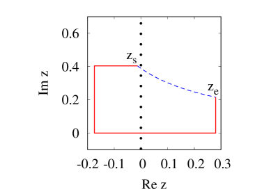
Figure 1: The $z$ integration path when the start and end points ($z_{\mathrm{s}}$ and $z_{\mathrm{e}}$) appear in the different quadrants. Closed circles represent singular points. The solid and dashed lines mean the integration path with and without our prescription, respectively.

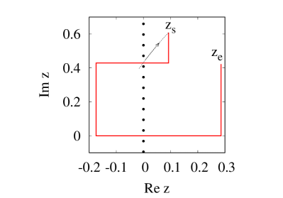
Figure 2: The $z$ integration path when $z_{\mathrm{s}}$ and $z_{\mathrm{e}}$ appear in the same quadrant. The arrow means the moving direction of the start position from Fig. 1 to present figure with the $t$-evolution of the gradient flow. Other symbols and lines are same with those in Fig. 1.

This prescription is imposed to fix the flow trajectories on the same Riemann sheet in the gradient-flow evolution since the value of the ${\tilde{p}}$-integration depends on the slit through which the path goes. In the naive Lefschetz thimble method without the prescription, the integration path in the complex $z$ plane becomes the dashed line in Fig. 1 and it provides wrong results.

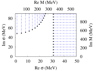
Figure 3: Structure of singular points and cuts in the complex $\sigma$ plane.

Figure 3 shows the structure of singular points and cuts in the complex $\sigma$ plane. It should be noted that we can set directions of cuts to a certain degree and thus present directions are just an example.

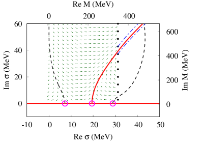
Figure 4: Lefschetz thimbles in the complex $\sigma$ plane. Open circles mean maximum and minima of the effective action, corresponding to $\tau=1,3,2$ respectively from the left. Solid and dashed lines represent ${\cal J}$ and ${\cal K}$ for each thimble, respectively. In the present case, ${\cal J}_{1,2}$ and ${\cal K}_{3}$ form same lines and thus we do no show ${\cal K}_{3}$ in the figure. Singular points are expressed by closed circles. Cuts are drawn by dot-dashed lines, but we here only draw nearest-neighbor cuts of ${\cal J}_{2}$.

The NJL model is the cutoff theory and thus the $|M|>\Lambda$ region does not matter, but some cuts exist inside the relevant region for the integration. This problem should be important in all $\mu$ region. Results are shown in Fig. 4. Present NJL model in the numerical calculation does not have the repulsive vector-current interaction and thus it does not have the auxiliary sign problem. We just use this model as an laboratory to check the singularity and cut effects for gradient flows. Actually, Lefschetz thimbles and the original integration-path become exactly the same in this case. Of course, it will be changed if we introduce the vector-current interaction.

In the present analysis, we analytically sum over the Matsubara frequencies and thus we encounter the difficulty of singular points and cuts. However, it is also true that we will encounter the same difficulty even in the case that Matsubara frequencies are not summed over analytically in the the coordinate-space representation because both path-integral formulations in the momentum- and coordinate-space representations are equivalent. In the lattice simulation, it is impossible to take the exact thermodynamic limit without the extrapolation and thus present singularity issue may be weaken, but it exists in principle. Therefore, numerical calculations are safe if configurations are localized far from the singularities, but not if configurations appear around the singularities. This problem should also appear in the complex Langevin method since the method also use the flow evaluation for performing the integration process. The difficulty from the singularities becomes more serious when the dimension of the space-time becomes larger and larger. Therefore, our analysis becomes important if we apply the Lefschetz-thimble path-integral method and the complex Langevin method to the four dimensional and also higher dimensional fermionic models.

5 Lefschetz thimble of Wick rotated vector field

We shall now discuss the Lefschetz thimble of the Wick rotated vector field. In the previous section, we have found that the thimble of the auxiliary scalar field is the same as the original integration path when the vector field is fixed to be zero. Then we do not have the sign problem. In the case where the vector field is switched on, the auxiliary sign problem may arise as discussed in the Introduction. We adopt the same prescription as in the scalar field case; the gradient flow trajectory is required to evolve on the same Riemann sheet.

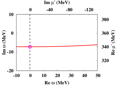
Figure 5: Lefschetz thimble in the complex $\omega_{4}$ plane. The solid and dashed lines show the downward and upward thimbles, ${\cal J}$ and ${\cal K}$, respectively, and the open circle shows the fixed point.

In Fig. 5, we show the Lefschetz thimble for the Wick rotated auxiliary vector field, $\omega$, at $T=10$ MeV and $\mu=360$ MeV. The scalar field, $\sigma,$ is small at this $(T,\mu)$ and is assumed to be zero. As expected, the $\omega_{4}$ takes the pure imaginary value at the fixed point, $\omega_{4}=-i\omega_{0}\simeq-i\langle q^{\dagger}q\rangle$, and the downward thimble runs approximately in parallel to the original integration path, the real axis. Thus, by constructing the integration path of the Wick rotated vector field in the complex plane, the auxiliary sign problem can be removed.

6 Summary

In this study, we have investigated the auxiliary sign problem which arises when the fermionic theory has the repulsive vector-field in variables of integration after the bosonization procedure: The Boltzmann weight in the partition function should oscillate by the repulsive vector-field when we make the path-integral well-define. If fermionic effective models do not have the sign problem and those path-integral are ill-defined after the simple bosonization procedure, the Wick rotation of the repulsive vector-field cures the illness. Necessity of this Wick rotation has been discussed in the detailed procedure of the bosonization. However, the Wick rotation induces the auxiliary sign problem. To explicitly discuss the auxiliary sign problem, we have used the two-flavor Nambu–Jona-Lasinio (NJL) model as an example. This model with the vector-current interaction dose not have the original sign problem, but its path-integral is ill-defined. The Wick rotation for the $\omega_{0}$ field which is induced from the repulsive vector-current interaction after the bosonization can make the path integral well-defined. However, the $\omega_{4}$ field induces the oscillating Boltzmann weight in the NJL partition function via the effective complex chemical potential. This auxiliary sign problem can be resolved by the Lefschetz-thimble path-integral method and then the effective action satisfy following relations;

$$\Gamma[z]\in\mathbb{R},~{}~{}~{}~{}\lim_{\omega_{4}\to\pm\infty}(-\Gamma[z])=-\infty.$$ (16)

Therefore, the path integral on the Lefschetz thimbles with the Wick rotation is well-defined and then the auxiliary sign problem vanishes.

However, after using the Wick rotation and the Lefschetz thimble method, we found that there are singular points and cuts induced by the square root and the logarithmic function in the momentum integration plane. These singularities sometimes induce the numerical instability for the gradient-flow evolution and we can not draw the Lefschetz thimble continuously. To analyze this problem, we consider the system which has either auxiliary scalar or vector fields. Then, we have proposed the new prescription for it by using the momentum integration in the complex domain to fix the gradient flow trajectories on the same Riemann sheet. In the prescription, choice of the integration path in the complexified momentum space is crucial.

This study is related with the sign problem and also the robustly defined path-integral formulation when the repulsive vector-field exists in variables of integration. The vector field is not a special concept in the path integral and thus present formulation should have wide application range in several quantum systems.

The authors thank Yoshimasa Hidaka and Yuya Nakagawa for helpful comments. A.O. is supported in part by the Grants-in-Aid for Scientific Research from JSPS (Nos. 15K05079, 15H03663, 16K05350), the Grants-in-Aid for Scientific Research on Innovative Areas from MEXT (Nos. 24105001, 24105008), and by the Yukawa International Program for Quark-hadron Sciences (YIPQS).

References

- [1] P. de Forcrand, Simulating QCD at finite density, PoS LAT2009 (2009) 010. arXiv:1005.0539.
- [2] Z. Fodor, S. Katz, A New method to study lattice QCD at finite temperature and chemical potential, Phys.Lett. B534 (2002) 87–92. arXiv:hep-lat/0104001, doi:10.1016/S0370-2693(02)01583-6.
- [3] Z. Fodor, S. Katz, Lattice determination of the critical point of QCD at finite T and mu, JHEP 0203 (2002) 014. arXiv:hep-lat/0106002, doi:10.1088/1126-6708/2002/03/014.
- [4] C. R. Allton, S. Ejiri, S. J. Hands, O. Kaczmarek, F. Karsch, E. Laermann, C. Schmidt, L. Scorzato, The QCD thermal phase transition in the presence of a small chemical potential, Phys. Rev. D66 (2002) 074507. arXiv:hep-lat/0204010, doi:10.1103/PhysRevD.66.074507.
- [5] C. Allton, M. Doring, S. Ejiri, S. Hands, O. Kaczmarek, et al., Thermodynamics of two flavor QCD to sixth order in quark chemical potential, Phys.Rev. D71 (2005) 054508. arXiv:hep-lat/0501030, doi:10.1103/PhysRevD.71.054508.
- [6] R. Gavai, S. Gupta, QCD at finite chemical potential with six time slices, Phys.Rev. D78 (2008) 114503. arXiv:0806.2233, doi:10.1103/PhysRevD.78.114503.
- [7] M.-P. Lombardo, Finite density (might well be easier) at finite temperature, Nucl. Phys. Proc. Suppl. 83 (2000) 375–377. arXiv:hep-lat/9908006, doi:10.1016/S0920-5632(00)91678-5.
- [8] P. de Forcrand, O. Philipsen, The QCD phase diagram for small densities from imaginary chemical potential, Nucl. Phys. B642 (2002) 290–306. arXiv:hep-lat/0205016, doi:10.1016/S0550-3213(02)00626-0.
- [9] M. D’Elia, M.-P. Lombardo, Finite density QCD via imaginary chemical potential, Phys.Rev. D67 (2003) 014505. arXiv:hep-lat/0209146, doi:10.1103/PhysRevD.67.014505.
- [10] E. Dagotto, A. Moreo, R. L. Sugar, D. Toussaint, Binding of Holes in the Hubbard Model, Phys. Rev. B41 (1990) 811–814. doi:10.1103/PhysRevB.41.811.
- [11] M. G. Alford, A. Kapustin, F. Wilczek, Imaginary chemical potential and finite fermion density on the lattice, Phys. Rev. D59 (1999) 054502. arXiv:hep-lat/9807039, doi:10.1103/PhysRevD.59.054502.
- [12] D. E. Miller, K. Redlich, Exact Implementation of Baryon Number Conservation in Lattice Gauge Theory, Phys. Rev. D35 (1987) 2524. doi:10.1103/PhysRevD.35.2524.
- [13] A. Hasenfratz, D. Toussaint, Canonical ensembles and nonzero density quantum chromodynamics, Nucl. Phys. B371 (1992) 539–549. doi:10.1016/0550-3213(92)90247-9.
- [14] G. Parisi, ON COMPLEX PROBABILITIES, Phys.Lett. B131 (1983) 393–395. doi:10.1016/0370-2693(83)90525-7.
- [15] J. R. Klauder, Coherent State Langevin Equations for Canonical Quantum Systems With Applications to the Quantized Hall Effect, Phys. Rev. A29 (1984) 2036–2047. doi:10.1103/PhysRevA.29.2036.
- [16] G. Aarts, E. Seiler, I.-O. Stamatescu, The Complex Langevin method: When can it be trusted?, Phys. Rev. D81 (2010) 054508. arXiv:0912.3360, doi:10.1103/PhysRevD.81.054508.
- [17] Z. Fodor, S. D. Katz, D. Sexty, C. Török, Complex Langevin dynamics for dynamical QCD at nonzero chemical potential: A comparison with multiparameter reweighting, Phys. Rev. D92 (9) (2015) 094516. arXiv:1508.05260, doi:10.1103/PhysRevD.92.094516.
- [18] J. Nishimura, S. Shimasaki, New Insights into the Problem with a Singular Drift Term in the Complex Langevin Method, Phys. Rev. D92 (1) (2015) 011501. arXiv:1504.08359, doi:10.1103/PhysRevD.92.011501.
- [19] E. Witten, Analytic Continuation Of Chern-Simons Theory, AMS/IP Stud. Adv. Math. 50 (2011) 347–446. arXiv:1001.2933.
- [20] M. Cristoforetti, F. Di Renzo, L. Scorzato, New approach to the sign problem in quantum field theories: High density QCD on a Lefschetz thimble, Phys.Rev. D86 (2012) 074506. arXiv:1205.3996, doi:10.1103/PhysRevD.86.074506.
- [21] H. Fujii, D. Honda, M. Kato, Y. Kikukawa, S. Komatsu, T. Sano, Hybrid Monte Carlo on Lefschetz thimbles - A study of the residual sign problem, JHEP 1310 (2013) 147. arXiv:1309.4371, doi:10.1007/JHEP10(2013)147.
- [22] F. Pham, Vanishing homologies and the variable saddlepoint method, in: Proc. Symp. Pure Math, no. 40, 1983, pp. 319–333. doi:http://dx.doi.org/10.1090/pspum/040.2.
- [23] S. E. Koonin, D. J. Dean, K. Langanke, Shell model Monte Carlo methods, Phys. Rept. 278 (1997) 1–77. arXiv:nucl-th/9602006, doi:10.1016/S0370-1573(96)00017-8.
- [24] H. Fujii, S. Kamata, Y. Kikukawa, Lefschetz thimble structure in one-dimensional lattice Thirring model at finite density, JHEP 11 (2015) 078, [Erratum: JHEP02,036(2016)]. arXiv:1509.08176, doi:10.1007/JHEP02(2016)036,10.1007/JHEP11(2015)078.
- [25] H. Fujii, S. Kamata, Y. Kikukawa, Monte Carlo study of Lefschetz thimble structure in one-dimensional Thirring model at finite density, JHEP 12 (2015) 125, [Erratum: JHEP09,172(2016)]. arXiv:1509.09141, doi:10.1007/JHEP12(2015)125,10.1007/JHEP09(2016)172.
- [26] A. Alexandru, G. Basar, P. F. Bedaque, G. W. Ridgway, N. C. Warrington, Monte Carlo calculations of the finite density Thirring model, Phys. Rev. D95 (1) (2017) 014502. arXiv:1609.01730, doi:10.1103/PhysRevD.95.014502.
- [27] W. E. Thirring, A Soluble relativistic field theory?, Annals Phys. 3 (1958) 91–112. doi:10.1016/0003-4916(58)90015-0.
- [28] A. Hasenfratz, P. Hasenfratz, K. Jansen, J. Kuti, Y. Shen, The Equivalence of the top quark condensate and the elementary Higgs field, Nucl. Phys. B365 (1991) 79–97. doi:10.1016/0550-3213(91)90607-Y.
- [29] J. Rantaharju, V. Drach, C. Pica, F. Sannino, The Nambu Jona-Lasinio model with Wilson fermionsarXiv:1609.08051.
- [30] J. Kubo, K. S. Lim, M. Lindner, Gamma-ray Line from Nambu-Goldstone Dark Matter in a Scale Invariant Extension of the Standard Model, JHEP 09 (2014) 016. arXiv:1405.1052, doi:10.1007/JHEP09(2014)016.
- [31] P. Channuie, C. Xiong, A unified composite model of inflation and dark matter in the Nambu-Jona-Lasinio theoryarXiv:1609.04698.
- [32] E. Nakano, T. Tatsumi, Chiral symmetry and density wave in quark matter, Phys.Rev. D71 (2005) 114006. arXiv:hep-ph/0411350, doi:10.1103/PhysRevD.71.114006.
- [33] D. Nickel, How many phases meet at the chiral critical point?, Phys.Rev.Lett. 103 (2009) 072301. arXiv:0902.1778, doi:10.1103/PhysRevLett.103.072301.
- [34] M. Fukuma, N. Umeda, Parallel tempering algorithm for the integration over Lefschetz thimblesarXiv:1703.00861.
- [35] K. Kashiwa, T. Hell, W. Weise, Nonlocal Polyakov-Nambu-Jona-Lasinio model and imaginary chemical potential, Phys.Rev. D84 (2011) 056010. arXiv:1106.5025, doi:10.1103/PhysRevD.84.056010.
- [36] K. Kashiwa, H. Kouno, T. Sakaguchi, M. Matsuzaki, M. Yahiro, Chiral phase transition in an extended NJL model with higher-order multi-quark interactions, Phys.Lett. B647 (2007) 446–451. arXiv:nucl-th/0608078, doi:10.1016/j.physletb.2007.01.061.