Lyapunov functions for a non-linear model of the X-ray bursting of the microquasar GRS 1915+105

Abstract

This paper introduces a biparametric family of Lyapunov functions for a non-linear mathematical model based on the FitzHugh-Nagumo equations able to reproduce some main features of the X-ray bursting behaviour exhibited by the microquasar GRS 1915+105. These functions are useful to investigate the properties of equilibrium points and allow us to demonstrate a theorem on the global stability. The transition between bursting and stable behaviour is also analyzed.

1 Introduction

The X-ray source GRS 1915+105, the prototype of microquasars, was discovered by Castro-Tirado et al. [1], and later identified with a binary system containing an accreting disk around a black hole by Mirabel and Rodríguez [2]. The X-ray emission is highly variable and characterised by a several different variability patterns, that alternate steady and noisy emission to series of bursts and dips. A first classification of the observed time behaviour based on the signal structure and on the photon energy distribution was presented by Belloni et al. [3], who defined twelve classes identified by a greek letter, but more patterns were observed on subsequent occasions. In particular, the variability class $\rho$ is characterised by series of bursts with a variable recurrence time and superposed to a rather stable level. The time profile of the bursts presents a rather smooth rising branch, the Slow Leading Trail (hereafter SLT), followed by a Pulse with a few intense and short peaks and a fast decline, as those shown in the upper panel of Fig. 1. The burst sequence was soon recognized as an evidence of a limit-cycle by Taam et al. [4] and explained by the occurrence in an physical parameters’ space, like the plane of the disk temperature $vs$ the integrated surface density, of an instability region where closed trajectories can be established (see, for instance, Taam & Lin [5], Lasota & Pelat [6], Mineshige [7], Szuszkiewicz & Miller [8]). However, the application of these models to observational results requires numerical solution of a complex system of non-linear partial differential equations taking into account several non-observable quantities in the viscous fluid dynamics and thermal processes in the accreting gas orbiting around a black hole. This approach makes hard to establish a simpler mathematical modelling of the source’s behaviour and the transition from a variability class to another. We therefore tried a different way based on a direct description of the observational data by means of mathematical models.

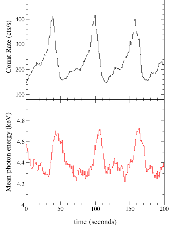
Figure 1: The top panel shows a short segment of the count rate time series in the entire MECS energy range during the October 2000 observation of BeppoSAX  [9]; the bottom panel presents the simultaneous changes of mean energy.

In a couple of papers, Massaro et al. [9] and Massa et al. [10] studied the time properties of a long series of bursts of GRS 1915+105 having a variable recurrence ranging time from 40 to more than 100 seconds. Massa et al. [10] developed an phase averaging algorithm to derive the burst mean profile and the mean photon energy curve which are shown in the left panel of Fig. 2. On this basis Massaro et al. [11] were able to describe this cycle by means of a modified FitzHugh-Nagumo (FitzHugh [12], Nagumo et al. [13]) model and found that it reproduces the mean burst shape and some other observational properties of the $\rho$ class. In the same paper [11] we also demonstrated that a limit cycle can exist and gave the conditions for the parameters to have this solution. It is given by the following system in the two dimensionless variables $x(t)$ and $y(t)$:

$$\left\{\begin{array}[]{lcl}dx/dt&=&-\rho x^{3}+\chi x-\gamma y-J\\ dy/dt&=&x-y\end{array}\right.$$ (1)

where

$$(i) ~{}~{}~{}~{}\rho,\chi,\gamma~{}and~{}J~{}are~{}positive~{}parameters$$

$$(ii) ~{}~{}~{}~{}\chi<\gamma+3(\rho J^{2}/4)^{1/3}~{}~{},~{}~{}\gamma>1$$ (2)

The parameter $J$ can be considered as an external forcing quantity, whereas $\rho$, $\chi$ and $\gamma$ can be related to the physical structure of the accreting disk.

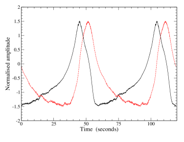
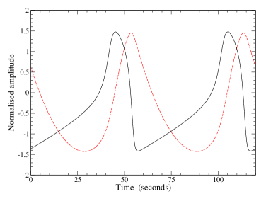
Figure 2: Left panel: time evolution of the mean pulse profile (black continuous line) and mean photon energy (red dashed line) of GRS 1915+105 in the $\rho$ class. Right panel: results obtained from numerical solution of the model of Eq. (1) with the parameters’ value given in the text, black continuous and red dashed lines represent the time behaviour of the $x$ and $y$ variables, respectively scaled as the curves in the left panel.

The success of  the system (1)  in reproducing  the GRS 1915+105

burst series depends on the presence of the cubic term that could be related to radiative energy dissipation of the accretion disk considering, for instance, that the black body photon emissivity is also proportional to the third power of the temperature. These equations, however, are not the unique for this goal: for instance, we verified that the use the exponent 5 instead of 3 in the non linear dissipation term gives also similar solutions. Moreover, as we showed in [11], the introduction of a slowly time variable $J(t)$, that requires at least an additional equation, makes possible to obtain solutions very similar to other variablity classes. The system (1) should therefore be considered as one of the simplest tool for mathematical description of the $\rho$ class bursting, whose properties depends upon the parameter $J$. In particular, our aim is to study under which conditions the solutions computed for different values of $J$ can be used for describing the transition to stable states, like those actually observed in GRS 1915+105.

In particular, the $\chi$ class of Belloni et al. [3] is a typical case in which the source X-ray flux remains nearly constant and that, according these authors, it is much more frequently observed the all the other ones. The main purpose of the present paper is to establish conditions for the global asymptotic stability of the system (1) and how to calculate the $J$ value corresponding to the transition from stability to bursting.

2 Numerical solutions for the bursting behaviour

Solutions of the system (1) were numerically computed by means of a Runge-Kutta fourth order integration routine [14] considering all the four parameters as constant, although they, at least in principle, could change in time with the physical state of the source. Our first aim was to obtain a set of parameters’ values for which the $x$ variable gave a satisfactory solution for the time signals. The comparison between the mean burst and energy profiles with the $x$ and $y$ curves is shown in the two panels of Fig. 2, where the observed data (left panel) and the results of numerical computations (right panel) are shown. All the curves, after subtraction of their central values, were normalised to have close amplitudes. The agreement, although not exact, is fully sastifactory considering the rather simple mathematical model. The adopted values of the four parameters were $\rho=0.30$, $\chi=33.0$, $\gamma=222.0$, $J=1100.0$.

A very important and unexpected finding of this solution (see [11]), is that the variable $y$ reproduces well the evolution of mean photon energy, that is related to the disk temperature. This finding makes stronger the heuristic meaning of the non-linear model and suggests a simple linear relation between the variable $x$ with the source luminosity $L$, or any other physical quantity proportional to it as the photon density in the emitting regions of the disk, and of $y$ with the mean energy of photons, otherwise the main features of both data series would not be so finely matched. This correspondence between the formal variables $x$, $y$ and the physical observable quantities, is also apparent from the $x,y$ plot (hereafter phase space plot) that results similar, except for the scale factors, to the count-rate vs mean energy plot studied by Massa et al. [10] (see also Fig. 14 in Janiuk & Czerny [15]).

Equilibrium points are the intersections of nullclines which are the curves given by equations for $(dx/dt)=(dy/dt)=0$, that for Eqs.(1) are:

$$\gamma y = -\rho x^{3}+\chi x-J$$

$$x = y$$ (3)

and that can be easily reduced to the cubic equation:

$$\varphi(x)=x^{3}+\frac{\gamma-\chi}{\rho}~{}x+\frac{J}{\rho}=0$$ (4)

Considering the parameters’ values given above there is a unique (negative) equilibrium point given by:

$$x_{*}=\sqrt[3]{-\frac{J}{2\rho}+\sqrt{\Big{(}\frac{J}{2\rho}\Big{)}^{2}+\Big{(}\frac{\gamma-\chi}{3\rho}\Big{)}^{3}}}~{}+~{}\sqrt[3]{-\frac{J}{2\rho}-\sqrt{\Big{(}\frac{J}{2\rho}\Big{)}^{2}+\Big{(}\frac{\gamma-\chi}{3\rho}\Big{)}^{3}}}$$ (5)

that, using the above parameters’ values, gives the numerical value $x_{*}=y_{*}=-$5.54891.

Note that for about all the $SLT$ the $x,y$ trajectory remains very close to the $x$ nullcline, and only after it approaches the other nullcline near the equilibrium point, the trajectory rapidly moves to the right to reach the $x$ maximum on the other branch of the cubic line and then it decreases very rapidly towards the minimum on the former branch.

A transition from bursting to a stable state is obtained in our model simply with a change of the $J$ value. We will show in Sect.4 how the changes of this parameter affect the stability of the solution and that these modifications can account for the observed variability of GRS 1915+105.

3 Stability analysis

3.1 Linear analysis

Consider the system (1) with the assumptions (2), there is only a unique real solution $x_{*}<0$ and therefore only one equilibrium point $(x_{*},y_{*})$, $y_{*}=x_{*}$, exists and because $x_{*}$ is the unique negative solution of the equation $\varphi(x)=0$, in the following we will use $x_{*}$ as parameter instead of $J$.

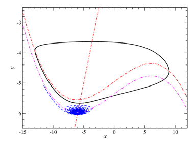
Figure 3: Phase space plot of the periodic solution of the system (1) computed using the same parameters’ values of curves Fig. 2. The loop is described in anti-clockwise direction as observed in the count-rate vs mean energy plots discussed by Massa et al. [10]. Red dash-dot lines are the nullclines for the Eqs (1). The violet dashed dot-dot line is the cubic equation for $J$=1190.6 and the dashed blue line is the corresponding solution of Eqs.(1), showing a trajectory approaching the stable equilibrium point.

For the study of the stability it is more convenient to define the two new variables:

$$u = x-x_{*}$$

$$v = (y-y_{*})-(x-x_{*})/\gamma$$ (6)

The system of differential equations becomes:

$$\left\{\begin{array}[]{lcl}du/dt&=&\gamma[f(u)-v]\\ dv/dt&=&g(u)\end{array}\right.$$ (7)

where defining $r=\rho/\gamma$    and    $a=3x_{*}^{2}+1/\rho-\chi/\rho$  it results

$$f(u)=-ru[u^{2}+3x_{*}u+a]$$ (8)

and

$$g(u)=ru[u^{2}+3x_{*}u+a+(1-1/\gamma)/r]~{}~{}~{}~{}.$$ (9)

Taking into account the conditions (2) we have

$$\gamma>1,r>0~{}~{},~{}~{}~{}x_{*}<0~{}~{},~{}~{}~{}x_{*}^{2}<(4/9)[a+(1-1/\gamma)/r]~{}~{}~{}~{}~{}~{}.$$ (10)

From the linear analysis [11, 16] one obtains the following results:

1) if $a>0$, $O(0,0)$ is locally asimptotically stable;
2) if $a<0$, $O(0,0)$ is unstable.

In the plane $(a,x_{*}^{2})$ (see Fig. 4), we  are inside  the region  defined by $a>-(1-1/\gamma)/r$ and $0<x_{*}^{2}<(4/9)[a+(1-1/\gamma)/r]$ and we consider the two regions A and B defined by the following open sets:

• A: $\{(a,x_{*}^{2})~{}|-(1-1/\gamma)/r<a<0,0<x_{*}^{2}<(4/9)[a+(1-1/\gamma)/r]\}$, in which there is a unique unstable equilibrium point;

• B: $\{(a,x_{*}^{2})~{}|a>0,0<x_{*}^{2}<(4/9)[a+(1-1/\gamma)/r]\}$, in which there is a unique locally asimptotically stable equilibrium point;

On the segment $x_{*}^{2}=(4/9)[a+(1-1/\gamma)/r]$ , $-(1-1/\gamma)/r<a<0$ there are two unstable equilibrium points, while on the half-line

$x_{*}^{2}=(4/9)[a+(1-1/\gamma)/r]$ , $a>0$

there are again two equilibrium points, one of which is unstable and the other one is locally asimptotically stable. The linear analysis, however, does not give information about the stability of the points on the segment with $a=0$.

3.2 Lyapunov function analysis

In [11] we demonstrated that if $(a,x_{*}^{2})\in{\bf A}$, there exist at least a limit cycle of (7) around the equilibrium point $O(0,0)$. In the following we demonstrate a general theorem to obtain sufficient conditions for the global asymptotic stability of the system (1). To this aim we introduce a family of biparametric Lyapunov functions that for this particular case generalizes the families introduced by Ardito & Ricciardi [17]. The proof is reached following La Salle & Lefschetz [18].   
  
Theorem 1:   Let us consider the system (7) where $f(\cdot)$ and $g(\cdot)$ are defined in (8) and (9), respectively, under the conditions (10). If $a\geq 0$ and if there exist $\tau,\nu\in\mathbb{R}_{+}\cup\{0\}$ such that

$$g(u)\cdot[e^{\nu\int_{0}^{u}g(s)ds}(\tau-f(u))-\tau]\geq 0$$ (11)

then it follows that $O(0,0)$ is a globally asimptotically stable equilibrium point.    

Proof.  Let

$$W_{\tau,\nu}:~{}~{}\mathbb{R}^{2}\to\mathbb{R}$$

and

$$W_{\tau,\nu}(u,v)=\int_{0}^{v}te^{\nu\gamma t(t/2-\tau)}dt+\frac{1}{\gamma}e^{\nu\gamma v(v/2-\tau)}\int_{0}^{u}g(t)e^{\nu\int_{0}^{t}g(s)ds}dt$$ (12)

obviously $W_{\tau,\nu}\in C^{1}(\mathbb{R}^{2},\mathbb{R})$ and $W_{\tau,\nu}(0,0)=0$.

Being $\gamma>1$ and $ug(u)>0$ $\forall u\neq 0$, it follows that

$W_{\tau,\nu}(u,v)>0~{}\forall~{}(u,v)\in\mathbb{R}^{2}-\{O(0,0)\}$     .

Moreover from the hypothesis (11) we get

$$\dot{W}_{\tau,\nu}(u,v)=-e^{\nu\gamma v(v/2-\tau)}g(u)[(\tau-f(u))e^{\nu\int_{0}^{u}g(s)ds}-\tau]\leq 0~{}~{}.$$ (13)

where $\dot{W}_{\tau,\nu}$ is the derivative of $W_{\tau,\nu}$ along the trajectories of the system (7); therefore $W_{\tau,\nu}$ is a Lyapunov function and $O(0,0)$ is stable.

In order to prove that $O(0,0)$ is globally asymptotically stable we observe that $W_{\tau,\nu}$ is radially unbounded, given that from (10)

$$\lim_{\parallel(u,v)\parallel\rightarrow+\infty}W_{\tau,\nu}(u,v)=+\infty~{},$$

thus the set

$$S_{l}=\{(u,v)\in\mathbb{R}^{2}|W_{\tau,\nu}(u,v)<l,l\in\mathbb{R}_{+}\}$$

is bounded.

Let

$$E=\{(u,v)\in S_{l}|\dot{W}_{\tau,\nu}(u,v)=0\}$$

being $\{O(0,0)\}$ the largest invariant set in $E$ the claim follows.

On the basis of this theorem it is possible to establish the following conditions for the global asymptotical stability.

Corollary 1:  Let us consider the system (7) where $f(\cdot)$ and $g(\cdot)$ are defined (8) and (9),respectively, under the conditions (10). If

$a\geq 0$,    and     $x_{*}^{2}<(4/9)a$

then $O(0,0)$ is globally asimptotically stable.

Proof.  In this case one has $u\cdot f(u)\leq 0$ and the thesis is a direct consequence of Th. 1 by taking $\tau=\nu=0$ in (12) and observing that the condition (11) is satisfied.   

Note that the family of Lyapunov functions given in (12), with the particular choice $\tau=\nu=0$ was introduced by Hsu [19]. This particular function, however, does not work in the analysis of the case for $a=0$ that corresponds to the transition between the regions of stablity and instability of the equilibrium point. For the study of this case we must consider again the Lyapunov function (12). Thus we have:   

Corollary 2:  Let us consider the system (7) where $f(\cdot)$ and $g(\cdot)$ are defined in (8) and (9), respectively, with the conditions given in (10). Let

$b\doteq a+(1-1/\gamma)/r$,

if

$a\geq 0$   and   $\frac{4}{9}a<x_{*}^{2}<\frac{b}{6}+\frac{ab}{9(a+b)}+\frac{1}{9}\sqrt{2ab}$

then $O(0,0)$ is globally asimptotically stable.

Proof.  We consider the function $W_{\tau,\nu}(u,v)$ defined by (12), then defining

$$S(u)\doteq e^{\nu\int_{0}^{u}g(s)ds}[\tau-f(u)]-\tau~{}~{}~{}~{}$$ (14)

we have that $\forall\tau,\nu>0$ it follows

$$\lim_{u\rightarrow-\infty}S(u)=-\infty~{}~{},~{}~{}\lim_{u\rightarrow+\infty}S(u)=+\infty~{}~{},~{}~{}S(0)=0$$ (15)

and

$$\frac{dS(u)}{du}=e^{\nu\int_{0}^{u}g(s)ds}~{}T(u)~{}~{}~{}~{},$$ (16)

where

$$T(u)=\nu g(u)(\tau-f(u))-f^{\prime}(u)~{}~{}~{}~{}.$$ (17)

With the choices $\tau=-3x_{*}(a+b)r$ and $\nu=2/rb(a+b)$, from the defintions of $f(u)$ and $g(u)$, one has

$$T(u) = \frac{2r}{b(a+b)}\Big{\{}u^{4}(u+3x_{*})^{2}+(a+b)[u^{4}+9u^{2}((ab/9)(a+b)+$$ (18)

$$+b/6-x_{*}^{2})+ab/2]\Big{\}}$$

From our assumptions it follows $T(u)\geq 0$, the condition (11) is satisfied and consequently the thesis is proved.

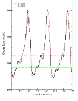
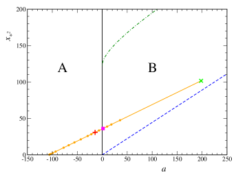
Figure 4: (Left panel: A short segment of the data of the same observation of those in the upper panel of Fig. 1 superposed to the solution of our mathematical model with $J=1100$ (red dash-dot curve). The two horizontal lines correspond to the signal levels calculated with $J=1200$ (magenta dotted line) and $J=2212$ to match the data of the observation of November 1996 when the source was in a stable state whose mean value is represented by the thick dashed green line. Right panel: Detail of the region in the $(a,x_{*}^{2})$ plane where is the solution for data modelling described in the text. The dashed blue line is given by the condition $x_{*}^{2}=(4/9)a$ and the green dash dotted curve corresponds to the upper limit for $x_{*}^{2}$. The orange continous line gives the locus of equilibrium points for different values of $J$, unstable in the region A and stable in region B, the red $\times$ marks the point corresponding to the red curve in the left panel, the magenta $\times$ corresponds to $J=1200$ and the green $\times$ gives the level observed in November 1996.

4 The transition from stable to unstable equilibrium

In addition to the description of the burst profiles of GRS 1915+105, the system (1) can be also used to study the transition to stable classes. Following Massaro et al. [11], we consider that $\rho$, $\chi$ and $\gamma$ remanin constant while the transition is driven by a slow change of $J$, that one can expect to be related with the accretion mass rate of the disk and then to its emission power.

The left panel of Fig. 4 shows the computed burst profile using the parameters’ values given in Sect. 2 together with a data segment in the energy range [1.6, 10] keV and the thick dashed green line indicates the mean level measured when the source was in the stable $\chi$ class observed by BeppoSAX. Let us observe that from the definition of $a=3x_{*}^{2}+1/\rho-\chi/\rho$ and from eq. (4) it results that

$$J=-x_{*}[a+(1-\frac{1}{\gamma})\frac{1}{r}-2x_{*}^{2}]~{}~{}~{}~{}.$$

The right panel shows a region in the plane $(a,x_{*}^{2})$ in which it is located the point corresponding to the model and the orange line tracks the locus of equilibrium points when $J$ increases from 100 (left lower extreme) to 2212 (right upper extreme). Notice that this line crosses the axis $a=0$ for the critical $J_{c}=1190.6$ at the transition point between unstable and stable equilibrium, in which the limit cycle converges soon to a constant value. This effect is illustrated in Fig. 3 by the blue lines: the dashed line is the nullcline for this critical value and the trajectory, computed using Eqs. (1), describes the global asymptotic stability of this point, as demonstrated in the previous section. Note that the orange line is entirely inside the region limited by the the dashed lines that are the limits for the application of the Cor. 2. Then all the solutions for $J>J_{c}$ are globally asymptotically stable and describe the $\chi$ class with a decreasing flux level for increasing $J$.

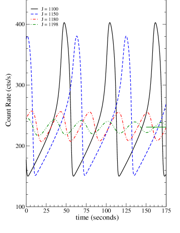
Figure 5: Evolution of the signal shape in the transition to stability: the black continuous curve is the one used to model the data and the other curves have been calculated for different values of $J$ on the two sides of the transition line. Note the changes of the amplitude and of the recurrence time approaching $J_{c}$, and for $J>J_{c}$ the progressive decrease of the amplitude towards the stable value, represented by the continuous horizontal segment on the right side.

We can investigate the changes of the signal for $J$ varying across the transition to stability. Some examples of burst pattern computed by means of our model are given in Fig. 5 in which we applied the same scale factors used for the left panel of Fig. 4. One can see that the amplitude of the signal has a fast decrease for $J$ just lower than the critical value, the burst profile is more symmetric without the sharp increase and the recurrence time becomes shorter. For $J$ just above $J_{c}$, a rather fast decay of the burst amplitude to the stable level, represented by the horizontal segment in Fig. 5, is apparent; higher values of $J$ correspond to faster decaying to the equilibrium. In these cases, however, because of the fast reaching of equilibrium, the resulting evolution of the signal is largely dependent on the initial values of the variables, and particularly, how much they differ form the equilibrium values.
A similar behaviour is obtained also for $y$, but considering the rather low amplitude of the observed modulation (about 10% in the lower panel of Fig. 1), a decrease to a few percent would require a very high instrumental sensitivity for a statistically significant detection.

The comparison of the class transition derived from the model with the observed behaviour of GRS 1915+105 is practically very hard because it requires the detection of the transition from the $\rho$ to the $\chi$ class. This transition depends on the rapidity of the $J$ variation and could occur in a rather short time, then the probability that an X-ray telescope on board an orbiting satellite is pointing at the source just in such an occasion is very low. In particular, no $\rho-\chi$ transition is observed in the entire BeppoSAX  data set considered in our analysis.

5 Conclusion

Non-linear dynamical models can be used for reproducing several interesting features of the time behaviour exhibited by the variable astrophysical source GRS 1915+105. In this paper we focused our interest on the study of stability of the solutions of the system proposed by Massaro et al. [11] for the $\rho$ class bursting and explored the transition between this and another class characterized by a stable emission. To this aim we introduced a biparametric Lyapunov function, that extends the previous results of Ardito & Ricciardi [17]. We found that, in the more physically interesting region of the parameters’ space, it is possible to have either an unstable equilibrium point, around which closed trajectories of limit cycle can be established, or equilibrium points, whose global asymptotical stable was demostrated in Corollary 2. The observed bursting behaviour of the source and the transition to stable states and vice versa, can be thus simply accounted for by changes of only the forcing parameter.

In the past years two other sources have been observed to exhibit a similar bursting pattern: IGR J17091+3624 (Altamirano et al. [20]), and the X-ray binary MXB 1730-335 (also known as Rapid Burster) very recently reported by Bagnoli & in’t Zand [21], the latter one with a long recurrence time of about 7 minutes, suggesting that it could be a phenomenon more frequent than considered in the past when GRS 1915+105 was the unique cosmic source. The approach presented here can be useful for developing general mathematical tools for modelling this complex quasi-periodic process in astrophysical sources and to obtain a description in terms of observable quantities of the accretion disk instabilities.

References

References

- [1] Castro-Tirado, A.J., Brandt, S. & Lund, N. GRS 1915+105, IAUC N. 5590 (1992).
- [2] Mirabel, I.F.& Rodriguez, L.F. A superluminal source in the Galaxy, Nature 371, 46 (1994).
- [3] Belloni, T., Klein-Wolt, M., Méndez, M. et al. A model-independent analysis of the variability of GRS 1915+105, Astron. Astrophys. 355, 271 (2000).
- [4] Taam, R.E., Chen, X., Swank, J.H., Rapid Bursts from GRS 1915+105 with RXTE, ApJ 485, L83 (1997).
- [5] Taam, R.E., Lin, D.N.C., The evolution of the inner regions of viscous accretion disks surrounding neutron stars, ApJ 287, 761 (1984).
- [6] Lasota, J.P., Pelat,D., Variability of accretion discs around compact objects, Astron. Astrophys. 249, 574 (1991).
- [7] Mineshige, S., Accretion disks instabilities, APSS 210, 83 (1993).
- [8] Szuszkiewicz, E., Miller, J.C., Limit-Cycle Behaviour of Thermally Unstable Accretion Flows on to Black Holes, MNRAS 298, 888 (1998).
- [9] Massaro, E., Ventura, G., Massa, F., Feroci, M. et al. The complex behaviour of the microquasar GRS 1915+105 in the class observed with BeppoSAX. I.Timing analysis Astron. Astrophys. 513, A21 (2010).
- [10] Massa, F., Massaro, E., Mineo, T. et al. The complex behaviour of the microquasar GRS 1915+105 in the class observed with BeppoSAX. III. The hard X-ray delay and limit cycle mapping Astron. Astrophys. 556, A84 (2013).
- [11] Massaro, E., Ardito, A., Ricciardi, P., Massa, F. et al. Non-linear oscillator models for the X-ray bursting of the microquasar GRS 1915+105, Astrophys. Space Sci. 352, 699-714 (2014).
- [12] FitzHugh, R. Impulses and Physiological States in Theoretical Models of Nerve Membrane Biophys. J. 1, 445, (1961).
- [13] Nagumo, J., Arimoto, S., Yoshizawa, S. An active pulse transmission line simulating nerve axon, Proc IRE 50, 2061 (1962).
- [14] Press, W.H., Teukolsky, S.A., Vetterling, W.T., Flannery, B.P. Numerical Recipes: The Art of Scientific Computing, Third Edition, Cambridge University Press (2007).
- [15] Janiuk, A., Czerny, B. Time-delays between the soft and hard X-ray bands in GRS 1915+105, MNRAS 356, 205 (2005).
- [16] Hahn, W. Stability of motion, Springer-Verlag, Berlin (1967).
- [17] Ardito, A., Ricciardi, P., Lyapunov functions for a generalized Gause-type model, J. Math. Biol. 33, 816 (1995)
- [18] La Salle, J., Lefshetz, S. Stability by Liapunov’s direct method with applications, Academic Press, New York (1961)
- [19] Hsu, S.B. On global stability of a predator-prey system, Math. Bosci 39, 1 (1978).
- [20] Altamirano, D., Belloni, T., Linares, M. et al., The Faint ”Heartbeats” of IGR J17091-3624: An Exceptional Black Hole Candidate, ApJ, 742, L17 (2011)
- [21] Bagnoli, T., in’t Zand, J.J.M., Discovery of GRS 1915+105 variability patterns in the Rapid Burster, MNRAS 450L, 52 (2015)