Spatial Random Sampling: A Structure-Preserving Data Sketching Tool

Abstract

Random column sampling is not guaranteed to yield data sketches that preserve the underlying structures of the data and may not sample sufficiently from less-populated data clusters. Also, adaptive sampling can often provide accurate low rank approximations, yet may fall short of producing descriptive data sketches, especially when the cluster centers are linearly dependent. Motivated by that, this paper introduces a novel randomized column sampling tool dubbed Spatial Random Sampling (SRS), in which data points are sampled based on their proximity to randomly sampled points on the unit sphere. The most compelling feature of SRS is that the corresponding probability of sampling from a given data cluster is proportional to the surface area the cluster occupies on the unit sphere, independently of the size of the cluster population. Although it is fully randomized, SRS is shown to provide descriptive and balanced data representations. The proposed idea addresses a pressing need in data science and holds potential to inspire many novel approaches for analysis of big data.

I Introduction

The complexity of many of the existing data analysis and machine learning algorithms limits their scalability to high-dimensional settings. This has spurred great interest in data sketching techniques that produce descriptive and representative sketches of the data on the premise that substantial complexity reductions can be potentially achieved without sacrificing performance when data inferencing is carried out using such sketches in lieu of the full-scale data [1, 2, 3, 4, 5, 6, 7, 8, 9, 10, 11, 12, 13].

Random embedding and random column sampling are two widely used linear data sketching tools. Random embedding projects data in a high-dimensional space onto a random low-dimensional subspace, and was shown to notably reduce dimensionality while preserving the pairwise distances between the data points [13, 14, 15]. While random embedding can generally preserve the structure of the data, it is not suitable for feature/column sampling. In random column sampling, a column is selected via random sampling from the column index set – hence the alternative designation Random Index Sampling (RIS). For RIS, the probability of sampling from a data cluster is clearly proportional to its population size. As a result, RIS may fall short of preserving structure if the data is unbalanced, in the sense that RIS may not sample sufficiently from less-populated data clusters, and/or may not capture worthwhile features that could be pertinent to rare events. This motivates the work of this paper in which we develop a new random sampling tool that can yield a descriptive data sketch even if the given data is largely unbalanced.

Over the last two decades, many different column sampling methods were proposed [16]. Most of these methods aim to find a small set of informative data columns whose span can well approximate the given data. In other words, if $\mathbf{C}\in\mathbb{R}^{N_{1}\times n}$ is the matrix of sampled columns, where $n$ is the number of sampled columns and $N_{1}$ the ambient dimension, most of the existing column sampling methods seek a solution to the optimization problem

$$\min_{\mathbf{C}}\>\>\|\mathbf{D}-\mathbf{C}\mathbf{C}^{\dagger}\mathbf{D}\|_{F},$$ (1)

where $\mathbf{D}\in\mathbb{R}^{N_{1}\times N_{2}}$ denotes the data, ^† the pseudoinverse, and $\|\cdot\|_{F}$ the Frobenius norm. These methods can be broadly categorized into randomized [17, 18, 19, 20, 21, 22, 23, 24] and deterministic methods [25, 26, 27, 28, 29, 30, 31, 32, 33]. In randomized methods, the columns are sampled based on a carefully chosen probability distribution. For instance, [23] uses the $\ell_{2}$-norm of the columns, and in [24] the sampling probabilities are proportional to the norms of the rows of the top right singular vectors. There are different types of deterministic sampling algorithms, including the rank revealing QR algorithm [33], and clustering-based algorithms [29]. In [32, 34, 35, 25], the non-convex optimization (1) is relaxed to a convex program by finding a row-sparse representation of the data. We refer the reader to [16, 36, 37] and references therein for more information about the matrix approximation based sampling methods.

Whereas low rank approximation has been instrumental in many applications, the sampling algorithms based on (1) cannot always guarantee that the sampled points satisfactorily capture the structure of the data. For instance, suppose the columns of $\mathbf{D}$ form $m$ clusters in the $N_{1}$-dimensional space, but the cluster centers are linearly dependent. An algorithm which aims to minimize (1) would not necessarily sample from each data cluster since it only looks for a set of columns whose span is that of the dominant singular vectors of $\mathbf{D}$.

For notation, bold-face upper-case letters denote matrices and bold-face lower-case letters denote vectors. Given a matrix $\mathbf{A}$, $\mathbf{a}_{i}$ and $\mathbf{a}^{i}$ denote its $i^{\text{th}}$ column and $i^{\text{th}}$ row, respectively. For a vector $\mathbf{a}$, $\max\mathbf{a}$ is its maximum element, $|\mathbf{a}|$ the vector of absolute values of its elements, and $\mathbf{a}_{\cal I}$ for an index set $\cal I$ the elements of $\mathbf{a}$ indexed by $\cal I$. Also, $\mathbb{S}^{N_{1}-1}$ designates the unit $\ell_{2}$-norm sphere in $\mathbb{R}^{N_{1}}$.

II Proposed Method

As mentioned earlier, with RIS the probability of sampling from a data cluster is proportional to its population size. However, in many applications of interest the desideratum is to collect more samples from clusters that occupy a larger space or that have higher dimensions, thereby composing a structure-preserving sketch of the data. For instance, suppose the data points lie on $\mathbb{S}^{N_{1}-1}$ and form two linearly separable clusters such that the surface area corresponding to the first cluster on the unit sphere is greater than that of the second cluster. In this case, a structure-preserving sketch should generally comprise more data points from the first cluster. However, RIS would sample more points from the cluster with the larger population regardless of the structure of the data.

II-A Spatially random column sampling

When the data points are projected onto $\mathbb{S}^{N_{1}-1}$, each cluster will occupy a certain surface area on the unit sphere. We propose a random column sampling approach in which the probability of sampling from a data cluster is proportional to its corresponding surface area. The proposed method, dubbed Spatially Random column Sampling (SRS), is presented in the table of Algorithm 1 along with the definitions of the used symbols. SRS samples the $n$ data points whose normalized versions have the largest projections along $n$ randomly selected directions in $\mathbb{R}^{N_{1}}$ (the rows of matrix $\mathbf{\Phi}$). Unlike RIS, SRS performs random sampling in the spatial domain as opposed to the index domain, wherefore the probability of sampling from a data cluster depends on its spatial distribution. To provide some insight into the operation of SRS, consider the following fact [38, 39].

Lemma 1.

If the elements of $\bm{\phi}\in\mathbb{R}^{N_{1}}$ are sampled independently from $\mathcal{N}(0,1)$, the vector $\bm{\phi}/\|\bm{\phi}\|_{2}$ will have a uniform distribution on the unit $\ell_{2}$-norm sphere $\mathbb{S}^{N_{1}-1}$.

According to Lemma 1, $\bm{\phi}^{i}/\|\bm{\phi}^{i}\|_{2}$ corresponds to a random point on the unit sphere (recalling that $\bm{\phi}^{i}$ is the $i^{\text{th}}$ row of $\mathbf{\Phi}$). The probability that a random direction lies in a given cluster is proportional to its corresponding surface area on the unit sphere. Since we cannot ensure if a random direction lies in a data cluster, we sample the data point at minimum distance from the randomly sampled direction. Therefore, Algorithm 1 samples $n$ points randomly on the unit sphere, and for each randomly sampled direction samples the data points with closest proximity to that direction. As such, it is more likely to sample from a data cluster that covers a larger area on the unit sphere. More precisely, suppose the columns of $\mathbf{D}$ have unit $\ell_{2}$-norm and form $s$ separable clusters. We divide the surface area of the unit sphere into $s$ regions $\{\mathcal{R}_{i}\}_{i=1}^{s}$, where $\mathcal{R}_{i}$ is defined as follows.

Definition 1.

Suppose the matrix $\mathbf{D}$ can be represented as $\mathbf{D}=[\mathbf{D}_{1}\>...\>\mathbf{D}_{s}]\mathbf{T}$, where $\mathbf{D}_{k}$ consists of the data points in the $k^{\text{th}}$ cluster, $\mathbf{T}$ is a permutation matrix, and the columns of $\mathbf{D}$ have unit $\ell_{2}$-norm. The region $\mathcal{R}_{i}$ is defined as

$$\mathcal{R}_{i}:=\left\{\mathbf{y}\in\mathbb{S}^{N_{1}-1}\Big{|}\max|\mathbf{y}^{T}\mathbf{D}_{i}|>\max|\mathbf{y}^{T}\mathbf{D}_{j}|,\>\forall\>j\neq i\right\}.$$

Accordingly, the probability of sampling a data point from the $k^{\text{th}}$ cluster is linear in the area of $\mathcal{R}_{k}$.

Remark 1.

Define $\mathbf{U}$ as an orthonormal basis for the column space of $\mathbf{D}$. Since the rows of $\mathbf{\Phi}$ are random vectors, $\mathbb{P}[\mathbf{U}^{T}\bm{\phi}^{i}=0]=0,\forall i$, where $\mathbb{P}$ denotes the probability measure. In addition, since $\bm{\phi}^{i}/\|\bm{\phi}^{i}\|_{2}$ has a uniform distribution on $\mathbb{S}^{N_{1}-1}$, $\mathbf{U}\mathbf{U}^{T}\bm{\phi}^{i}/\|\mathbf{U}^{T}\bm{\phi}^{i}\|_{2}$ has a uniform distribution on the intersection of the column space of $\mathbf{U}$ and $\mathbb{S}^{N_{1}-1}$. Thus, SRS generates $n$ random directions in the span of the data.

In the following section, we compare the requirements of RIS and SRS (as two completely random column sampling tools) using a set of theoretical examples.

Algorithm 1 Spatially random column sampling (SRS without replacement)

Input: Data matrix $\mathbf{D}\in\mathbb{R}^{N_{1}\times N_{2}}$ and $n$ as the number of sampled columns.

Initialization: Construct matrix $\mathbf{\Phi}\in\mathbb{R}^{n\times N_{1}}$ by sampling independently from $\mathcal{N}(0,1)$. Set $\mathbf{Y}$ equal to an empty matrix.

1. Data Normalization: Define $\mathbf{X}\in\mathbb{R}^{N_{1}\times N_{2}}$ such that $\mathbf{x}_{i}=\mathbf{d}_{i}/\|\mathbf{d}_{i}\|_{2}$.

2. Column Sampling:
2.1 Set $\mathbf{Q}=\mathbf{\Phi}\mathbf{X}$ and set $\mathcal{I}=\emptyset$.

2.2 For $i=1$ to $n$
2.2.1 Define $\mathbf{h}=\left|\mathbf{q}^{i}\right|$ and set $\mathbf{h}_{\mathcal{I}}=0$.
2.2.2 Define $\mathbf{x}_{k}$ as the $k^{\text{th}}$ column of $\mathbf{X}$, where $k$ is the index of the maximum element of $\mathbf{h}$.
2.2.3 Update $\mathbf{Y}=[\mathbf{Y}\>\>\mathbf{x}_{k}]$ and add $k$ to the set $\mathcal{I}$.
2.2 End For

Output: $\mathbf{Y}\in\mathbb{R}^{N_{1}\times n}$ is the matrix of sampled columns.

Algorithm 2 SRS with replacement

1. Perform step 1 of Algorithm 1 and set $\mathbf{Q}=\mathbf{\Phi}\mathbf{X}$.

2. Column Sampling: Matrix $\mathbf{Y}\in\mathbb{R}^{N_{1}\times n}$ is the matrix of sampled columns. The $i^{\text{th}}$ column of $\mathbf{Y}$, $\mathbf{y}_{i}$, is equal to $\mathbf{x}_{k}$ where $k$ is equal to the index of the maximum element of $|\mathbf{q}^{i}|$.

II-B Sample complexity analysis

This section provides a theoretical analysis of the sample complexity of SRS in the context of two examples, in which we show that the probability of sampling from a data cluster with SRS can be independent of the cluster population. The sample complexity is contrasted to that of conventional RIS. To simplify the analysis, we assume that sampling in SRS is done with replacement (c.f. Algorithm 2).

Figure 1: Left: The distribution of data in a two-dimensional space. The data consists of two clusters shown in yellow. The normalized points in the first and second clusters are distributed on two separate arcs with lengths $\tau_{1}$ and $\tau_{2}$, respectively. Each of the two arcs does not overlap with the image of the other arc w.r.t. the origin on the unit circle. Right: The rank of randomly sampled columns by RIS and SRS versus the number of sampled columns.

Example 1: Suppose $N_{1}=2$ and the columns of $\mathbf{X}$ lie in two spatially separate clusters. The data distribution is illustrated in the left plot of Fig. 1. The data points lie on two separate arcs of the unit $\ell_{2}$-norm circle with lengths $\tau_{1}$ and $\tau_{2}$. We further assume that each of the two arcs does not overlap with the image of the other arc w.r.t. the origin on the unit circle. The number of data points in the first and second clusters are equal to $n_{1}$ and $n_{2}$, respectively. The following two lemmas compare the number of columns sampled randomly by RIS and SRS required to ensure that at least $m$ data points are sampled from each cluster, where $m<\min\{n_{1},n_{2}\}$.

Lemma 2.

Suppose $N_{1}=2$ and the distribution of the data columns follows the assumptions of Example 1. Assume $\beta\geq 2+\frac{3}{m}\log\frac{4}{\delta}$. If the number of columns sampled by RIS with replacement is greater than $\beta m\frac{N_{2}}{\min_{i}\{n_{i}\}},$ then the number of data points sampled from each data cluster is greater than or equal to $m$, with probability at least $1-\delta$.

Lemma 3.

Suppose $N_{1}=2$, the distribution of the data columns follows the assumptions of Example 1 as in Fig. 1 , $\beta\geq 2+\frac{3}{m}\log\frac{4}{\delta},$ and $\tau_{2}+\tau_{1}<\pi$. If the number of columns sampled by SRS (with replacement) is greater than $\beta m\frac{2\pi}{\pi-|\tau_{2}-\tau_{1}|}\>,$ then the number of data points sampled from each data cluster is greater than or equal to $m$, with probability at least $1-\delta$.

Lemma 2 establishes a sufficient condition on the number of columns sampled by RIS, which is shown to be linear in $\frac{N_{2}}{\min_{i}n_{i}}$ since with RIS the probability of sampling from the $i^{\text{th}}$ cluster is $n_{i}/N_{2}$. Thus, if the populations of the data clusters are unbalanced (i.e., not of the same order), we will need to sample a large number of points to ensure the sampled columns are descriptive, i.e., enough points are drawn from every cluster. On the other hand, Lemma 3 shows that the sufficient number of columns sampled by SRS is independent of the cluster populations since the probabilities of sampling from the first and the second clusters with SRS are equal to $\frac{\pi+\tau_{1}-\tau_{2}}{2\pi}$ and $\frac{\pi+\tau_{2}-\tau_{1}}{2\pi}$, respectively. These sampling probabilities are proportional to the surface areas covered by the clusters on the unit sphere (c.f. Definition 1) independently from the cluster populations.

Example 2: In this example, we consider a different clustering structure in which the columns of the data matrix $\mathbf{D}$ lie in a union of $s$ linear subspaces (the subspace clustering structure [40, 41]). Assumption 1 formalizes the underlying data model.

Assumption 1.

The columns of $\mathbf{D}$ lie in a union of $s$ random $(r/s)$-dimensional linear subspaces. i.e., $\mathbf{D}=[\mathbf{U}_{1}\mathbf{Q}_{1}\>...\>\mathbf{U}_{s}\mathbf{Q}_{s}]$, where $\mathbf{Q}_{i}\in\mathbb{R}^{r/s\times n_{i}}$, $n_{i}$ is the number of data points in the $i^{\text{th}}$ subspace, and $\mathbf{U}_{i}\in\mathbb{R}^{N_{1}\times r/s}$ is an orthonormal basis for the $i^{\text{th}}$ subspace. The data points in each subspace are distributed uniformly at random, $\sum_{i=1}^{s}n_{i}=N_{2}$, and $\underset{i}{\min}\>{n_{i}}\gg r/s$.

Define $\{p_{i}\}_{i=1}^{s}$ as the sampling probabilities from the data clusters. The following lemma provides a sufficient condition on the number of randomly sampled columns to ensure that they span the column space of $\mathbf{D}$.

Lemma 4.

Suppose Assumption 1 holds, the rank of $\mathbf{D}$ is equal to $r$, and RIS or SRS is used to sample $n$ columns (with replacement). If

$$n\geq\frac{1}{\underset{i}{\min}\>p_{i}}\>\xi_{\max}\left(2+\frac{3}{\xi_{\min}}\log\frac{2\>s}{\delta}\right),$$ (2)

then the sampled columns span the column space of $\mathbf{D}$ with probability at least $1-2\delta-2\sum_{i=1}^{s}n_{i}^{-3}$, where $\xi_{\min}={10}\>c\>{\max(r/s,\log\underset{i}{\min}\>n_{i})}\log\frac{2r}{\delta}$, $\xi_{\max}={10}\>c\>{\max(r/s,\log\underset{i}{\max}\>n_{i})}\log\frac{2r}{\delta}$, and $c$ is a real constant.

Thus, the sufficient number of sampled columns using RIS and SRS is of order $\mathcal{O}(\frac{r}{\underset{i}{\min}\>p_{i}})$. With RIS, $\underset{i}{\max}\>1/p_{i}=N_{2}/\underset{i}{\min}\>n_{i}$. Hence, if the data is unbalanced, the sample complexity of RIS is high. If we use SRS for column sampling, the probability of sampling from the $i^{\text{th}}$ cluster is equal to

$$\mathbb{P}\left[\max|\phi^{T}\mathbf{U}_{i}\mathbf{Q}_{i}|>\underset{j\neq i}{\max}\left(\max|\phi^{T}\mathbf{U}_{j}\mathbf{Q}_{j}|\right)\right].$$

In contrast to RIS where the sampling probability solely depends on the population ratio, in SRS it also depends on the structure of the data. We show that if the data follows Assumption 1 and the number of data points in each subspace is sufficiently large, the probability of sampling from a data cluster can be independent of the population ratio. Before stating this result in Lemma 5, we define $i^{{}^{\prime}}:=\operatorname*{arg\,min}n_{i}$, and define,

$$p(\epsilon,s)=\mathbb{P}\left[\|\phi^{T}\mathbf{U}_{i^{{}^{\prime}}}\|_{2}^{2}>(1+\epsilon)\>\underset{i\neq i^{{}^{\prime}}}{\max}\|\phi^{T}\mathbf{U}_{i}\|_{2}^{2}\right],$$

for some $\epsilon>0$. If $\epsilon$ is sufficiently small, $p(\epsilon,s)$ is approximately equal to $1/s$. For instance, if $s=2$, the distribution of $x=\|\phi^{T}\mathbf{U}_{1}\|_{2}^{2}/\|\phi^{T}\mathbf{U}_{2}\|_{2}^{2}$ is the F-distribution $f(x;r/2,r/2)$ and $f(1;r/2,r/2)=1/2$ [42].

Lemma 5.

For any $0<\delta<1$, there exits an integer $\hat{n}_{\delta}$ such that if $n_{i^{{}^{\prime}}}>\hat{n}_{\delta}$, then $p_{i^{{}^{\prime}}}>p(\epsilon,s)(1-\delta)$.

Per Lemma 5, the probability of sampling from a subspace can be independent from the population ratio given there are enough data points in the subspaces, i.e., the probability of sampling from a data cluster can be arbitrarily close to $1/s$ even if ${{\min_{i}n_{i}}}/{N_{2}}$ is close to zero. Note that this does not mean that each subspace should have a large number of data points for SRS to yield a descriptive data sketch. For instance, suppose $\mathbf{D}$ follows Assumption 1 with $r=100$, $s=50$, $\{n_{i}\}_{i=1}^{25}=20$, and $\{n_{i}\}_{i=26}^{50}=500$ (The data lies in the union of 50 2-dimensional subspaces, $\underset{i}{\min}\>n_{i}=20$, and $N_{2}/\underset{i}{\min}\>n_{i}=25$). The right plot of Fig. 1 shows the rank of randomly sampled columns versus the number of sampled columns. RIS samples about 4000 columns to capture the column space versus 200 columns for SRS.

II-C Balanced sketching

A marked feature of SRS is that the sampling probabilities depend on the spatial distribution of the data. Therefore, even when the distribution of the data is highly unbalanced, SRS can yield balanced data sketches. For instance, suppose the data follows the distribution shown in the left plot of Fig. 1 with $\tau_{1}=\tau_{2}$. Since $\tau_{1}=\tau_{2}$, SRS samples a number of points of the same order from each cluster with high probability. Therefore, the data sketch obtained by SRS is balanced even if the given data is not. This feature is crucial in big data analysis. As an example, consider a scenario where $n_{1}\gg n_{2}$. If some data clustering algorithm is applied to identify two cluster centers, it will select both centers from the first cluster (thus fails to recognize the underlying data structure) as it seeks to minimize the distances between the data points and the cluster centers. However, if the clustering algorithm is applied to a data sketch obtained through SRS, it can identify appropriate cluster centers since SRS balances the distribution of the data in the sketch.

II-D Computational complexity

The computational complexity of SRS can be reduced by applying Algorithm 1 to a sketch of the rows of $\mathbf{D}$. Define matrix $\mathbf{D}^{{}^{\prime}}\in\mathbf{R}^{p\times N_{1}}$ as $\mathbf{D}^{{}^{\prime}}=\mathbf{S}\mathbf{D}$. We consider three choices for the matrix $\mathbf{S}$. One choice is where the rows of $\mathbf{S}$ are a random subset of the standard basis, which amounts to random row sampling. However, a sufficient number of rows should be sampled to ensure that the underlying structures are preserved. If the sampling algorithm is applied to $\mathbf{D}^{{}^{\prime}}$ obtained by row sampling, the complexity is reduced from $O(nN_{1}N_{2})$ to $O(npN_{2})$. The second choice is to select $\mathbf{S}$ from sparse random embedding matrices [43, 44]. Since a sparse random embedding matrix contains many zeros, a much reduced number of multiplications is needed to perform the random embedding step akin to random row sampling. The third choice is to use a matrix $\mathbf{S}$ with entries that are independent binary random variables ($\pm 1$ with equal probability). Random embedding using such a matrix does not involve any numerical multiplications and was shown to yield embedding performance that closely approaches that of random Gaussian matrices [14]. Algorithm 1 can be applied to $\mathbf{D}^{{}^{\prime}}$ since the embedding matrix $\mathbf{S}$ preserves the essential information in $\mathbf{D}$.

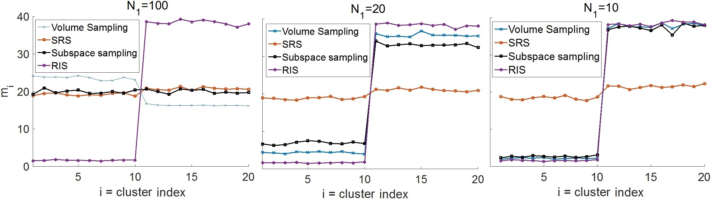
Figure 2: The number of sampled columns from each data cluster for different values of $N_{1}$.

II-E Discussion and conclusion

This paper proposed a new random data sketching tool, which carries out the random sampling in the spatial domain. We emphasize that SRS is not meant to be a replacement for, nor a modification to, RIS. Rather, it is a new sketching tool which has its own applicability. We showed that SRS can provide a balanced data sketch and has higher chance of sampling from rare events compared to sampling with RIS. Unlike matrix approximation based methods which require the cluster centers to be independent, linear independence is not important for SRS.

III Numerical Experiments

In this section, we present a set of numerical experiments using both synthetic and real data to showcase the effectiveness of SRS in preserving the underlying data structure.

III-A Balanced data sketching

Suppose the data follows the subspace clustered structure in Assumption 1 with $r=40$, $s=20$, $\{n_{i}\}_{i=1}^{10}=30$, and $\{n_{i}\}_{i=11}^{20}=700$. Thus, the columns of $\mathbf{D}$ lie in a union of 20 2-dimensional linear subspaces and the distribution of the data is quite unbalanced. The distribution of the data points in the sketch obtained by SRS is compared to that obtained by RIS and by two other adaptive column sampling methods, namely, subspace sampling [24] and volume sampling [45, 17]. We sample a total of 400 columns. For the subspace sampling method, we use $\min(r,N_{1})$ right singular vectors to compute the sampling probabilities. Volume sampling is an iterative column sampling method that samples one column at a time. It projects the data on the complement space of the sampled data points, thus stops sampling after roughly $\hat{r}$ steps, where $\hat{r}$ is the rank of data. In this experiment, we apply volume sampling multiple times to sample 400 data columns (in each time the sampled columns are removed from the data).

Fig. 2 shows the number of data points $m_{i}$ sampled from each data cluster as a function of the cluster index $i=1,\ldots,20$. The plots are obtained by averaging over 100 independent runs. If $N_{1}>40$, the subspaces are independent with high probability. Clearly, when $N_{1}=100>40$, almost all the sampling algorithms can yield a balanced data sketch except for RIS. However, as $N_{1}$ decreases (e.g., $N_{1}=10$ and $N_{1}=20$), the subspaces are no longer independent. In this case, only SRS is shown to yield a balanced data sketch. This is due to the fact that the sampling probability with RIS depends on the sizes of the populations of the clusters, and adaptive sampling only guarantees that the span of the sampled columns well approximates the column space of the data.

III-B Spatially fair random sampling

Similar to the previous subsection, assume the data lie in a union of 20 linear subspaces $\{\mathcal{S}\}_{i=1}^{20}$. The dimension of subspaces $\{\mathcal{S}\}_{i=1}^{10}$ is equal to 2 and the dimension of subspaces $\{\mathcal{S}\}_{i=11}^{20}$ is equal to 4. The number of data points lying in each of the subspaces $\{\mathcal{S}\}_{i=1}^{10}$ is equal to 3200, while the number of data points lying in each of the subspaces $\{\mathcal{S}\}_{i=11}^{20}$ is only 80. Thus, $N_{2}=\left(10\times 80+10\times 3200\right)$. Importantly, the subspaces with the lower dimension contain 40 times more data points than those with the higher dimension. Since more data points are required to represent clusters with higher dimensions, we naturally desire that the sampling algorithm samples more points from such clusters. In this experiment, 300 data columns are sampled. Fig. 3 shows the average number of data points sampled from each cluster. In the left plot, $\mathbf{D}\in\mathbb{R}^{100\times N_{2}}$. Thus, the subspaces are independent with high probability. One can observe that all the sampling algorithms except RIS follow a similar pattern of sampling, namely, sample more data points from the 10 subspaces with the higher dimensions.

In the middle and right plots, the sampling algorithms are applied to a sketch of the data obtained by randomly embedding the data into a lower dimension space. The sampling algorithms are applied to $\mathbf{D}^{{}^{\prime}}=\mathbf{S}\mathbf{D}$, where in the middle plot $\mathbf{S}\in\mathbb{R}^{20\times N_{1}}$ and in the right plot $\mathbf{S}\in\mathbb{R}^{10\times N_{1}}$ and $N_{1}=100$. The matrix $\mathbf{S}$ is a random binary matrix whose elements are independent random variables with values $\pm 1$ with equal probability. One can observe that only SRS exhibits the same sampling pattern of the left plot. Since the matrix approximation based methods seek a good approximation of the dominant left singular vectors of the data, they cannot recognize the underlying clustering structure of the data if the clusters are linearly dependent.

III-C Column sampling for classification

We test the proposed approach with real data, the MNIST database [46]. The data consists of $28\times 28$ handwritten digit images. The MNIST database contains 50000 and 10000 images for training and testing, respectively, and 10000 images of validation data. In this experiment, we consider a binary classification problem. The first class corresponds to numbers between 0 to 4, and the second class corresponds to numbers greater than or equal to 5. The training data $\textbf{Tr}_{1}$ corresponding to the first class is constructed as $\textbf{Tr}_{1}=[\mathbf{D}_{0}\>\>\mathbf{D}_{1}\>\>\mathbf{D}_{2}\>\>\mathbf{D}_{3}\>\>\mathbf{D}_{4}]$, where $\mathbf{D}_{0}\in\mathbb{R}^{784\times 4900}$, $\mathbf{D}_{1}\in\mathbb{R}^{784\times k}$, $\mathbf{D}_{2}\in\mathbb{R}^{784\times 4900}$, $\mathbf{D}_{3}\in\mathbb{R}^{784\times k}$, $\mathbf{D}_{4}\in\mathbb{R}^{784\times 4900}$ ($k$ is a changing parameter as shown in Table I). The columns of $\mathbf{D}_{0}$, $\mathbf{D}_{1}$, $\mathbf{D}_{2}$, $\mathbf{D}_{3}$, and $\mathbf{D}_{4}$, are randomly sampled training images corresponding to digits 0, 1, 2, 3, and 4, respectively. Similarly, the training data corresponding to the second class is $\textbf{Tr}_{2}=[\mathbf{D}_{5}\>\>\mathbf{D}_{6}\>\>\mathbf{D}_{7}\>\>\mathbf{D}_{8}\>\>\mathbf{D}_{9}]$, where $\mathbf{D}_{5}\in\mathbb{R}^{784\times 4900}$, $\mathbf{D}_{6}\in\mathbb{R}^{784\times k}$, $\mathbf{D}_{7}\in\mathbb{R}^{784\times 4900}$, $\mathbf{D}_{8}\in\mathbb{R}^{784\times k}$, $\mathbf{D}_{9}\in\mathbb{R}^{784\times 4900}$. The columns of $\mathbf{D}_{5}$, $\mathbf{D}_{6}$, $\mathbf{D}_{7}$, $\mathbf{D}_{8}$, and $\mathbf{D}_{9}$, are randomly sampled training images corresponding to digits 5, 6, 7, 8, and 9, respectively. Thus, the entire training data is $\textbf{Tr}=[\textbf{Tr}_{1}\>\>\textbf{Tr}_{2}]$.

We do not use all the columns of Tr to train the classifier, rather we sample 1000 columns randomly from each class (2000 in total) and use these sampled columns to train the classifier. The classifier is a two-layer fully connected neural network with 400 neurons in each layer. Table 1 compares the classification accuracy for different values of $k$. When $k$ is small, the distribution of the data is unbalanced across classes. As shown the performance gap of RIS relative to SRS increases as $k$ decreases. For instance, when $k=300$, the classification accuracy achieved based on SRS is substantially higher by about 5 percent.

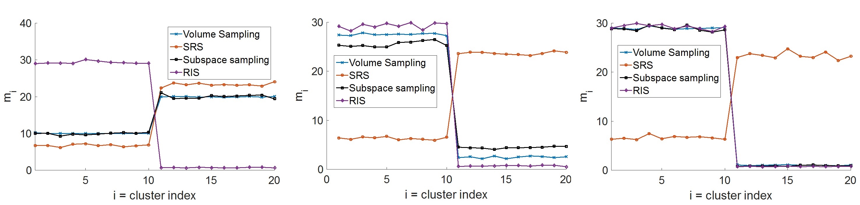
Figure 3: The number of columns sampled from each data cluster. In the left plot, the sampling algorithms are applied directly to the data. In the middle and right plot, the sampling algorithms are applied to a sketch of the data obtained through random embedding.

TABLE I: Classification accuracy of the classifier

Sampling method / $k$	4900	2000	1000	300
SRS	0.9671	0.9615	0.9587	0.9436
RIS	0.9615	0.9561	0.9443	0.8968

References

- [1] M. W. Mahoney and P. Drineas, “CUR matrix decompositions for improved data analysis,” Proceedings of the National Academy of Sciences, vol. 106, no. 3, pp. 697–702, 2009.
- [2] F. Woolfe, E. Liberty, V. Rokhlin, and M. Tygert, “A fast randomized algorithm for the approximation of matrices,” Applied and Computational Harmonic Analysis, vol. 25, no. 3, pp. 335–366, 2008.
- [3] J. Sun, Y. Xie, H. Zhang, and C. Faloutsos, “Less is more: Compact matrix decomposition for large sparse graphs,” in Proceedings of the SIAM International Conference on Data Mining, 2007, pp. 366–377.
- [4] P.-G. Martinsson, A. Szlam, and M. Tygert, “Normalized power iterations for the computation of SVD,” NIPS Workshop on Low-rank Methods for Large-scale Machine Learning, 2010.
- [5] R. H. Affandi, A. Kulesza, E. B. Fox, and B. Taskar, “Nystrom approximation for large-scale determinantal processes.” in AISTATS, 2013, pp. 85–98.
- [6] M. Rahmani and G. K. Atia, “High dimensional low rank plus sparse matrix decomposition,” IEEE Transactions on Signal Processing, vol. 65, no. 8, pp. 2004–2019, April 2017.
- [7] N. Halko, P.-G. Martinsson, Y. Shkolnisky, and M. Tygert, “An algorithm for the principal component analysis of large data sets,” SIAM Journal on Scientific computing, vol. 33, no. 5, pp. 2580–2594, 2011.
- [8] M. Rahmani and G. Atia, “Randomized robust subspace recovery and outlier detection for high dimensional data matrices,” IEEE Transactions on Signal Processing, vol. 65, no. 6, March 2017.
- [9] C. Boutsidis, A. Zouzias, and P. Drineas, “Random projections for -means clustering,” in Advances in Neural Information Processing Systems, 2010, pp. 298–306.
- [10] A. K. Farahat, A. Elgohary, A. Ghodsi, and M. S. Kamel, “Greedy column subset selection for large-scale data sets,” Knowledge and Information Systems, vol. 45, no. 1, pp. 1–34, 2015.
- [11] C. Boutsidis, P. Drineas, and M. W. Mahoney, “Unsupervised feature selection for the -means clustering problem,” in Advances in Neural Information Processing Systems, 2009, pp. 153–161.
- [12] A. Rahimi, B. Recht et al., “Random features for large-scale kernel machines,” in Advances in Neural Information Processing Systems, 2007, pp. 1177–1184.
- [13] N. Ailon and B. Chazelle, “Approximate nearest neighbors and the fast Johnson-Lindenstrauss transform,” in Proceedings of the thirty-eighth annual ACM symposium on Theory of computing, 2006, pp. 557–563.
- [14] D. Achlioptas, “Database-friendly random projections: Johnson-Lindenstrauss with binary coins,” Journal of computer and System Sciences, vol. 66, no. 4, pp. 671–687, 2003.
- [15] W. B. Johnson and J. Lindenstrauss, “Extensions of Lipschitz mappings into a Hilbert space,” Contemporary math., vol. 26, no. 189-206, 1984.
- [16] N. Halko, P.-G. Martinsson, and J. A. Tropp, “Finding structure with randomness: Probabilistic algorithms for constructing approximate matrix decompositions,” SIAM review, vol. 53, no. 2, pp. 217–288, 2011.
- [17] A. Deshpande, L. Rademacher, S. Vempala, and G. Wang, “Matrix approximation and projective clustering via volume sampling,” in Proc. of the 17th annual ACM-SIAM symposium on Discrete Algorithms. Society for Industrial and Applied Mathematics, 2006, pp. 1117–1126.
- [18] N. H. Nguyen, T. T. Do, and T. D. Tran, “A fast and efficient algorithm for low-rank approximation of a matrix,” in Proceedings of the forty-first annual ACM symposium on Theory of computing, 2009, pp. 215–224.
- [19] C. Boutsidis, M. W. Mahoney, and P. Drineas, “An improved approximation algorithm for the column subset selection problem,” in Proceedings of the twentieth Annual ACM-SIAM Symposium on Discrete Algorithms. Society for Industrial and Applied Mathematics, 2009, pp. 968–977.
- [20] M. Rudelson and R. Vershynin, “Sampling from large matrices: An approach through geometric functional analysis,” Journal of the ACM (JACM), vol. 54, no. 4, p. 21, 2007.
- [21] V. Guruswami and A. K. Sinop, “Optimal column-based low-rank matrix reconstruction,” in Proceedings of the twenty-third annual ACM-SIAM symposium on Discrete Algorithms. SIAM, 2012, pp. 1207–1214.
- [22] S. Paul, M. Magdon-Ismail, and P. Drineas, “Column selection via adaptive sampling,” in Advances in Neural Information Processing Systems, 2015, pp. 406–414.
- [23] P. Drineas, A. Frieze, R. Kannan, S. Vempala, and V. Vinay, “Clustering large graphs via the singular value decomposition,” Machine learning, vol. 56, no. 1-3, pp. 9–33, 2004.
- [24] P. Drineas, M. W. Mahoney, and S. Muthukrishnan, “Subspace sampling and relative-error matrix approximation: Column-based methods,” in Approximation, Randomization, and Combinatorial Optimization. Algorithms and Techniques. Springer, 2006, pp. 316–326.
- [25] M. Rahmani and G. Atia, “Robust and scalable column/row sampling from corrupted big data,” arXiv preprint arXiv:1611.05977, 2016.
- [26] L. Balzano, R. Nowak, and W. Bajwa, “Column subset selection with missing data,” in NIPS workshop on low-rank methods for large-scale machine learning, vol. 1, 2010.
- [27] A. K. Farahat, A. Ghodsi, and M. S. Kamel, “Efficient greedy feature selection for unsupervised learning,” Knowledge and information systems, vol. 35, no. 2, pp. 285–310, 2013.
- [28] A. Civril and M. Magdon-Ismail, “Column subset selection via sparse approximation of SVD,” Theoretical Computer Science, vol. 421, pp. 1–14, 2012.
- [29] C. Boutsidis, J. Sun, and N. Anerousis, “Clustered subset selection and its applications on IT service metrics,” in Proc. of the 17th ACM conf. on Information and knowledge management, 2008, pp. 599–608.
- [30] D. Lashkari and P. Golland, “Convex clustering with exemplar-based models,” Advances in neural information processing systems, vol. 20, 2007.
- [31] E. Esser, M. Moller, S. Osher, G. Sapiro, and J. Xin, “A convex model for nonnegative matrix factorization and dimensionality reduction on physical space,” IEEE Transactions on Image Processing, vol. 21, no. 7, pp. 3239–3252, 2012.
- [32] E. Elhamifar, G. Sapiro, and R. Vidal, “See all by looking at a few: Sparse modeling for finding representative objects,” in IEEE Conference on Computer Vision and Pattern Recognition, 2012, pp. 1600–1607.
- [33] M. Gu and S. C. Eisenstat, “Efficient algorithms for computing a strong rank-revealing QR factorization,” SIAM Journal on Scientific Computing, vol. 17, no. 4, pp. 848–869, 1996.
- [34] I. Misra, A. Shrivastava, and M. Hebert, “Data-driven exemplar model selection,” in IEEE Winter Conference on Applications of Computer Vision (WACV), 2014, pp. 339–346.
- [35] F. Nie, H. Huang, X. Cai, and C. H. Ding, “Efficient and robust feature selection via joint -norms minimization,” in Advances in Neural Information Processing Systems, 2010, pp. 1813–1821.
- [36] A. Deshpande and L. Rademacher, “Efficient volume sampling for row/column subset selection,” in 51st Annual IEEE Symposium on Foundations of Computer Science (FOCS), 2010, pp. 329–338.
- [37] E. Elhamifar, G. Sapiro, and R. Vidal, “Finding exemplars from pairwise dissimilarities via simultaneous sparse recovery,” in Advances in Neural Information Processing Systems, 2012, pp. 19–27.
- [38] T. T. Cai, J. Fan, and T. Jiang, “Distributions of angles in random packing on spheres,” Journal of Machine Learning Research, vol. 14, no. 1, pp. 1837–1864, 2013.
- [39] T. T. Cai and T. Jiang, “Phase transition in limiting distributions of coherence of high-dimensional random matrices,” Journal of Multivariate Analysis, vol. 107, pp. 24–39, 2012.
- [40] R. Vidal, “Subspace clustering,” IEEE Signal Processing Magazine, vol. 28, no. 2, pp. 52–68, 2011.
- [41] M. Rahmani and G. Atia, “Innovation pursuit: A new approach to subspace clustering,” ICML 2017, arXiv preprint arXiv:1512.00907, 2015.
- [42] A. M. Mood, Introduction to the Theory of Statistics. McGraw-hill, 1974.
- [43] D. M. Kane and J. Nelson, “Sparser Johnson-Lindenstrauss transforms,” Journal of the ACM (JACM), vol. 61, no. 1, 2014.
- [44] A. Dasgupta, R. Kumar, and T. Sarlós, “A sparse Johnson-Lindenstrauss transform,” in Proceedings of the forty-second ACM symposium on Theory of computing, 2010, pp. 341–350.
- [45] A. Deshpande and L. Rademacher, “Efficient volume sampling for row/column subset selection,” in 51st Annual IEEE Symposium on Foundations of Computer Science (FOCS), 2010, pp. 329–338.
- [46] Y. LeCun and C. Cortes, “MNIST handwritten digit database,” 2010. [Online]. Available: http://yann.lecun.com/exdb/mnist/