Gluing Ladders into Fishnets

Abstract

We use integrability at weak coupling to compute fishnet diagrams for four-point correlation functions in planar $\phi^{4}$ theory. The results are always multi-linear combinations of ladder integrals, which are in turn built out of classical polylogarithms. The Steinmann relations provide a powerful constraint on such linear combinations, leading to a natural conjecture for any fishnet diagram as the determinant of a matrix of ladder integrals.

I Introduction and Main Result

Integrability is a powerful tool for exploring theories such as planar ${\cal N}=4$ super-Yang-Mills (SYM) theory at finite coupling Beisert2010jr ; Basso2013vsa ; Gromov2013pga ; Basso2015zoa ; Fleury2016ykk ; Eden2016xvg . It can also assist in the computation of individual Feynman diagrams, in scalar theories directly Zamolodchikov1980mb ; Isaev2003tk , or after suitably twisting the SYM theory Gurdogan2015csr ; Caetano2016ydc ; Chicherin2017cns , or, more implicitly, through the “hexagonalization” of correlation functions Fleury2016ykk .

The Steinmann relations Steinmann provide stringent analytic constraints on multi-particle scattering amplitudes by forbidding double discontinuities in overlapping channels. They have been applied extensively in the multi-Regge limit, e.g. in refs. Stapp1982mq ; Bartels2008ce . Their far-reaching consequences outside of this limit were recognized more recently. Combined with the dual conformal symmetry of scattering amplitudes in the SYM theory, they severely restrict the types of functions that can appear, making it possible to bootstrap the six-point amplitude to five loops CaronHuot2016owq and the (symbol of the) seven-point amplitude to four loops Dixon2016nkn with very little additional input.

In this Letter, we combine integrability and the Steinmann relations in order to find a simple (conjectural) result for the doubly-infinite class of Feynman graphs depicted in fig. 1. They belong to a broader family of conformal integrals which has attracted much attention over the years Usyukina1993ch ; Broadhurst1993ib ; Drummond2006rz ; Broadhurst2010ds ; Drummond2013nda ; Eden2016dir ; Drummond2012bg ; Schnetz2013hqa ; Golz2015rea . The black lines in the figure provide the position-space interpretation of the “fishnet” diagram, as a contribution to the correlation function $G_{m,n}(x_{i})=\langle\phi_{2}^{n}(x_{1})\phi_{2}^{\dagger n}(x_{2})\phi_{1}^{m}(x_{3})\phi_{1}^{\dagger m}(x_{4})\rangle$, at weak coupling, $g^{2}\equiv\lambda/(4\pi)^{2}\ll 1$, with $\phi_{1,2}$ two orthogonal complex scalars, $\phi_{1,2}^{\dagger}$ their complex conjugates, and with $\lambda=g_{\rm YM}^{2}N_{c}$ the ’t Hooft coupling.

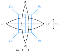
Figure 1: Fishnet diagram in $\phi^{4}$ theory and its dual off-shell (color-ordered) scattering amplitude.

We are only interested in the first planar graph contributing to this correlator. Given the $R$-charge assignment, all lines must cross each other, as in fig. 1 with the scalars’ quartic coupling $\lambda/(2\pi)^{4}=g^{2}/\pi^{2}$ (cf. the 10-point graph considered in ref. CaronHuot2012ab ). After integrating $\int d^{4}x_{k}$ over each intersection point $x_{k}$, $k>4$, and extracting a factor of the disconnected free propagators, this very first contribution to the correlator reads

$$G_{m,n}(x_{i})=\frac{g^{2mn}}{(x_{12}^{2})^{n}(x_{34}^{2})^{m}}\times\Phi_{m,n}(u,v)\,,$$ (1)

where $x_{ij}=x_{i}-x_{j}$. The two conformal cross ratios are

$$u=\frac{x_{14}^{2}x_{23}^{2}}{x_{12}^{2}x_{34}^{2}}\equiv\frac{z\bar{z}}{(1-z)(1-\bar{z})}\,,\,\,v=\frac{x_{13}^{2}x_{24}^{2}}{x_{12}^{2}x_{34}^{2}}\equiv\frac{u}{z\bar{z}}\,.$$ (2)

Alternatively, we could use the strongly twisted theory considered in refs. Gurdogan2015csr ; Caetano2016ydc ; Chicherin2017cns . In that theory, the gluons and fermions are decoupled, the correlator (1) is a particular instance of the off-shell amplitudes discussed in ref. Chicherin2017cns , and fig. 1 is the only diagram contributing to it.

The blue lines in fig. 1 indicate a dual-graph, or “momentum-space” (but not Fourier-transformed), interpretation of the quantity as a contribution to a scattering amplitude with four external massive momenta, $p_{1}=x_{23}$, $p_{2}=x_{31}$, $p_{3}=x_{14}$, $p_{4}=x_{42}$, and all massless internal lines. The Steinmann relations Steinmann forbid double discontinuities in the overlapping channels $(p_{1}+p_{2})^{2}=x_{12}^{2}$ and $(p_{2}+p_{3})^{2}=x_{34}^{2}$. The momentum-space interpretation looks like $m$ ladders glued together. The ladder integrals, corresponding to $m=1$, were computed long ago Usyukina1993ch in terms of classical polylogarithms. They also belong to a class of iterated integrals called single-valued harmonic polylogarithms (SVHPLs) BrownSVHPLs with weight (number of iterated integrations) equal to $2n$, where $n$ is the loop number. The ladder integrals are the building blocks for the fishnet integrals.

We find that $\Phi_{m,n}(u,v)$ can be written, for $m\leq n$, as

$$\Phi_{m,n}(u,v)=\bigg{[}\frac{(1-z)(1-\bar{z})}{z-\bar{z}}\bigg{]}^{m}I_{m,n}(z,\bar{z})\,,$$ (3)

where $I_{m,n}$ is an iterated integral (also known as a pure function) of weight $2mn$. It is symmetric under $3\leftrightarrow 4$ (equivalently, $u\leftrightarrow v$, or $z,\bar{z}\leftrightarrow 1/z,1/\bar{z}$) and under $z\leftrightarrow\bar{z}$, up to a sign,

$$I_{m,n}(1/z,1/\bar{z})=I_{m,n}(\bar{z},z)=(-1)^{m}I_{m,n}(z,\bar{z})\,.$$ (4)

Our main result is that $I_{m,n}$ is the determinant of an $m\times m$ matrix,

$$I_{m,n}=\textrm{det}\,M,\qquad M_{ij}=c_{ij}\,L_{n-m-1+i+j}\,.$$ (5)

The matrix elements are $1\times p$ ladder integrals $L_{p}$ (see eq. (16)) multiplied by rational numbers,

$$c_{ij}=\begin{cases}1,&i=j,\\ \prod_{k=j+1}^{i}p_{k}(p_{k}-1),\quad&i>j,\\ [c_{ji}|_{n\rightarrow n+j-i}]^{-1},&i<j,\end{cases}$$ (6)

where $p_{k}=n-m-1+j+k$. In the following, we discuss how integrability and analyticity lead to eq. (5).

II Pentagons, hexagons, and all that

In this section, we present two matrix-model-like integral representations for the diagram in fig. 1, using the integrability of planar SYM theory. They correspond to two different ways of factorizing the fishnet diagram, using the so-called flux-tube picture Alday2007mf ; Basso2013vsa , where the operators are inserted along the edges of a null Wilson loop, or the more recent approach proposed to study three- Basso2015zoa and higher-point functions Fleury2016ykk ; Eden2016xvg .

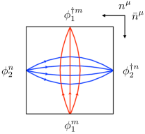
Figure 2: The correlator can be put inside a null square Wilson loop, with $x_{4}^{\mu}=n^{\mu},x^{\mu}_{2}=\bar{n}^{\mu},\bar{n}x_{3}=-e^{2\sigma_{1}},nx_{1}=-e^{-2\sigma_{2}}$, and $n^{2}=\bar{n}^{2}=0,n\cdot\bar{n}=1$. Moving $\phi_{1,2}$ along the edges is the same as changing the cross ratios $z=-e^{2\sigma_{1}}$ and $\bar{z}=-e^{-2\sigma_{2}}$.

Flux tube picture. In the flux tube picture (fig. 2) the two cross ratios map to the positions $\sigma_{1,2}$ of the operators along two light-like directions, $z=-e^{2\sigma_{1}},\bar{z}=-e^{-2\sigma_{2}}$. The correlator is viewed as a scattering of two beams on top of the Gubser-Klebanov-Polyakov GKP background. The beams are labelled by the scalars’ rapidities, $\textbf{u}=\{u_{1},\ldots,u_{m}\},\textbf{v}=\{v_{1},\ldots,v_{n}\}$, which are conjugate to shifts in $\sigma_{1}$ and $\sigma_{2}$, respectively, and are separately conserved throughout the entire process, thanks to integrability. The form factor for the creation and absorption of a beam at the boundary of the square, or equivalently the absolute value of the beam’s wave function, can be parametrized in terms of pentagon transitions $P$ Basso2013vsa :

$$\mu(\textbf{u};\sigma_{1})=\prod_{i=1}^{m}\mu(u_{i})e^{2iu_{i}\sigma_{1}}\prod_{i<j}^{m}\frac{1}{P(u_{i}|u_{j})P(u_{j}|u_{i})}\,,$$ (7)

with $\mu(u)=\pi\,\textrm{sech}{(\pi u)}$ and $P(u|v)=\Gamma(iu-iv)/\Gamma(\tfrac{1}{2}+iu)\Gamma(\tfrac{1}{2}-iv)$. Integrating (7) over the rapidities gives back the free propagator for $m$ scalar fields inserted along the null direction,

$$d(\sigma_{1})^{-m}=\bigg{[}\frac{1}{e^{\sigma_{1}}+e^{-\sigma_{1}}}\bigg{]}^{m}=\int\frac{d\textbf{u}}{m!}\,\mu(\textbf{u};\sigma_{1})\,,$$ (8)

with $d\textbf{u}=\prod_{i}du_{i}/(2\pi)$ and $\mathcal{h}\sqrt{-z}\phi(x_{3})\,\phi^{\dagger}(x_{4})\mathcal{i}=\sqrt{-z}/(1-z)=1/d(\sigma_{1})$. Eq. (8) is also the spin-chain scalar product in the so-called separated variables Derkachov2002tf . The same expression with $u_{i}\rightarrow v_{i}$, $m\rightarrow n$, $\sigma_{1}\rightarrow\sigma_{2}$ describes the second beam.

An essential property of flux-tube scattering is that it is diffractionless and fully factorized. Hence, the $m\times n$ grid in the diagram can be immediately taken into account by inserting $\prod_{i=1}^{m}\prod_{j=1}^{n}S_{\star}(u_{i},v_{j})$, where $S_{\star}(u,v)$ is the transmission part of the mirror two-body $S$-matrix Basso2013pxa ,

$$S_{\star}(u,v)=\frac{\pi g^{2}\sinh{(\pi(u-v))}}{(u-v)\cosh{(\pi u)}\cosh{(\pi v)}}\,.$$ (9)

The overall process is of order $O(g^{2mn})$, in agreement with the corresponding Feynman diagram.

Assembling all factors together, and dropping the powers of the coupling, we obtain the flux tube representation

$$\frac{\Phi_{m,n}}{d_{1}^{m}d_{2}^{n}}=\int\frac{d\textbf{u}d\textbf{v}}{m!n!}\prod_{i}^{m}\mu(u_{i})^{m+n}e^{2iu_{i}\sigma_{1}}\prod_{i}^{n}\mu(v_{i})^{m+n}e^{2iv_{i}\sigma_{2}}$$ (10)

$$\qquad\qquad\times\prod_{i<j}^{m}\Delta(u_{i},u_{j})\prod_{i,j}^{m,n}\tilde{\Delta}(u_{i},v_{j})\prod_{i<j}^{n}\Delta(v_{i},v_{j}),$$

where $d\textbf{v}=\prod_{i}dv_{i}/(2\pi)$, $d_{i}=d(\sigma_{i})$,

$$\tilde{\Delta}(u,v)=\frac{\sinh{(\pi(u-v))}}{\pi(u-v)}=\frac{\Delta(u,v)}{(u-v)^{2}}\,,$$ (11)

and dividing by the disconnected propagators matches the normalization (3). A similar integral has been used to study 2-to-2 fermion flux-tube scattering Basso2014koa .

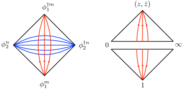
Figure 3: We can decompose the correlator using triangles (also known as hexagons). The red beam is made of $m$ magnons, produced on the bottom triangle and absorbed on the top one. The correlator is the scalar product between the two wave functions.

BMN picture. An alternative representation for the same correlator comes from the Berenstein-Maldacena-Nastase (BMN) BMN picture. In this picture, one beam, $\phi_{2}^{n}$, describes a reference state, the BMN vacuum, while the other, $\phi_{1}^{m}$, is viewed as a collection of $m$ magnons propagating through it. The latter are not the familiar magnons describing spin waves on top of the (ferromagnetic) vacuum, but some “mirror” versions of them, mapping to insertions along the direction $(x_{1},x_{2})=(0,\infty)$ of the reference beam, see fig. 3. Each magnon $\phi_{1}$ is further decomposed into partial waves with respect to dilatation and rotation, $z=\rho e^{i\phi}$; each carries a rapidity $u\in\mathbb{R}$ and bound state index $a\in\mathbb{Z}$ conjugate to these symmetries. The planar correlator is cut halfway by the vacuum into two triangles, which are naturally associated with three-point functions. The amplitudes for production and absorption of $m$ magnons on the two triangles can be obtained in terms of the so-called hexagon form factors Basso2015zoa ; Basso2015eqa . The next crucial ingredient is the rule for rotating each partial wave from a triangle ending on the reference points (0, 1, $\infty$) to the reference points $(0,z,\infty)$ Fleury2016ykk . Combining the two yields the wave-function overlap

$$\mu_{\textbf{a}}(\textbf{u};z)=\frac{|z|^{m}}{(z-\bar{z})^{m}}\prod_{i=1}^{m}z^{-iu_{i}+\tfrac{a_{i}}{2}}\bar{z}^{-iu_{i}-\tfrac{a_{i}}{2}}\mu_{a_{i}}(u_{i})\prod_{i<j}^{m}p_{ij}\,,$$ (12)

with $(\textbf{u},\textbf{a})=\{(u_{1},a_{1}),\ldots\}$, $\mu_{a}(u)=ag^{2}/(u^{2}+\tfrac{a^{2}}{4})^{2}$, $p_{ij}=p_{a_{i}a_{j}}(u_{i},u_{j})$, $p_{ab}(u,v)=\mu_{a}(u)\Delta_{ab}(u,v)\mu_{b}(v)/(ab)$, and $\Delta_{ab}(u,v)$ as defined in eq. (15) below.

Finally, the “scattering” between the magnons and the vacuum results in a factor $(g^{2}/(u^{2}+a^{2}/4))^{\ell}$ per magnon, where $\ell$ is the so-called bridge length. Naively, $\ell=n$, since there are $n$ vacuum lines to cross. In fact $m$ of these lines have been pulled out and included in the wave function (12), as shown in fig. 4 for $m=1$. This subtlety of the cutting explains why the wave function (12) is suppressed by $2m^{2}$ powers of the coupling and why the bridge length is $\ell=n-m$. For $n=0$ ($\ell=-m$), the overlap gives back the tree result, upon integration,

$$\sum_{\textbf{a}\in\mathbb{Z}^{m}}\int\frac{d\textbf{u}}{m!}\,\mu_{\textbf{a}}(\textbf{u};z)\prod_{i}^{m}\frac{(u_{i}^{2}+\tfrac{a_{i}^{2}}{4})^{m}}{g^{2m}}=\frac{|z|^{m}}{|1-z|^{2m}}\,,$$ (13)

with $|z|/|1-z|^{2}=\sqrt{x^{2}_{3}x^{2}_{4}}/x_{34}^{2}$ the scalar propagator in the conformal frame of fig. 3 (with the numerator absorbing the weights of the field).

Putting everything together, and normalizing by the disconnected correlator, eq. (13), leads to an integral for the pure function directly,

$$I_{m,n}=\sum_{\textbf{a}}\int\frac{d\textbf{u}}{m!}\prod_{i=1}^{m}\frac{a_{i}z^{-iu_{i}+a_{i}/2}\bar{z}^{-iu_{i}-a_{i}/2}}{(u_{i}^{2}+a_{i}^{2}/4)^{m+n}}\prod_{i<j}^{m}\Delta_{ij}\,,$$ (14)

with $\Delta_{ij}=\Delta_{a_{i}a_{j}}(u_{i},u_{j})$ and

$$\Delta_{ab}(u,v)=\biggl{[}(u-v)^{2}+\frac{(a-b)^{2}}{4}\biggr{]}\biggl{[}(u-v)^{2}+\frac{(a+b)^{2}}{4}\biggr{]}\,.$$ (15)

For $m=1$, this is the formula for the one magnon contribution to the four point function of chiral primary operators in planar $\mathcal{N}=4$ SYM Fleury2016ykk .

Analysis. The flux tube and BMN matrix integrals provide two formulae for the fishnet diagram which are equivalent, in principle. In practice, it is much easier to evaluate the latter. There are far fewer residues and the answer appears in closed form almost immediately; the final sum over the bound state labels is always expressible in terms of classical polylogarithms. The infinite series of ladder integrals ($m=1$) was easily reproduced in this manner Fleury2016ykk . Thanks to the polynomial nature of the magnon interaction, eq. (15), the fishnet diagrams are equally straightforward for reasonable values of $m,n$. We derived the result (5) through $m,n=1,\ldots,4$. We double-checked the answer against the flux-tube predictions for the few lowest residues when $m=2$. The main structural property, embodied in eq. (5), is that the fishnet diagrams are sums of products of $m$ ladder integrals. This observation is the seed for the Steinmann bootstrap program.

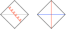
Figure 4: By supersymmetry, the measure $\mu_{a}(u)$ describes both the one-loop gluon diagram, on the left, and the one-loop scalar cross diagram, on the right. To get a free propagator, we must deconvolute the scalar diagram, by acting with the box operator $\Box/g^{2}=-z\bar{z}\partial_{z}\partial_{\bar{z}}/g^{2}$ or, equivalently, by introducing the form factor $(u^{2}+a^{2}/4)/g^{2}$ in rapidity space. A similar rule was used Basso2013vsa ; Belitsky2014sla ; Basso2015rta to transpose between MHV and NMHV amplitudes, in the flux tube picture. In general, the conversion is achieved through inclusion of a factor $((u^{2}+a^{2}/4)/g^{2})^{m}$, per excitation, where $m$ is the “NMHV” degree, or number of scalars at the cusp. This is readily seen to correct the mismatch between $\ell$ and $n$.

III Ladders, Steinmann, and all that

The ladder function $L_{p}$ is defined for $p>0$ by Usyukina1993ch ; Broadhurst2010ds

$$L_{p}=\sum_{j=p}^{2p}\frac{j!\ [-\ln(z\bar{z})]^{2p-j}}{p!(j-p)!(2p-j)!}[{\rm Li}_{j}(z)-{\rm Li}_{j}(\bar{z})],$$ (16)

and the tree-level value is $L_{0}=(z-\bar{z})/[(1-z)(1-\bar{z})]$. In the neighborhood of the origin in $z$, the polylogarithms ${\rm Li}_{j}(z)$ are analytic, and $L_{p}$ is manifestly single-valued, a real analytic funtion of $z$. That is, $L_{p}$ has no branch cuts under rotating $z\rightarrow ze^{2\pi i}$, $\bar{z}\rightarrow\bar{z}e^{-2\pi i}$. It does have (multiple) discontinuities in $z\bar{z}$: under $z\rightarrow ze^{\pi i}$, $\bar{z}\rightarrow\bar{z}e^{\pi i}$, the logarithm shifts by $\ln(z\bar{z})\rightarrow\ln(z\bar{z})+2\pi i$.

What is not so obvious from the representation (16) is that $L_{p}$ is also single-valued in $z$ around $z=1$. In fact it lies in the class of SVHPLs ${\cal L}_{\vec{w}}$ BrownSVHPLs ,

$$L_{p}=(-1)^{p}\Bigl{[}{\cal L}_{0,\ldots,0,1,0,0,\ldots,0}-{\cal L}_{0,\ldots,0,0,1,0,\ldots,0}\Bigr{]}\,,$$ (17)

where there are $p-1$ ($p$) 0’s before the 1 in the first (second) term, and $2p$ entries in all.

Now $L_{p}$ does have a discontinuity in $(1-z)(1-\bar{z})$: under $(1-z)\rightarrow(1-z)e^{\pi i}$, $(1-\bar{z})\rightarrow(1-\bar{z})e^{\pi i}$,

$$L_{p} \rightarrow L_{p}+{\rm Disc}_{1}L_{p}\,,$$ (18)

$${\rm Disc}_{1}L_{p} = 2\pi i\frac{(-1)^{p}}{p!(p-1)!}\,\ln(z/\bar{z})\,(\ln z\ln\bar{z})^{p-1}\,.$$ (19)

This discontinuity is compatible with the differential equation obeyed by $L_{p}$ Drummond2006rz :

$$z\bar{z}\partial_{z}\partial_{\bar{z}}L_{p} = -L_{p-1}\,,$$ (20)

$$z\bar{z}\partial_{z}\partial_{\bar{z}}{\rm Disc}_{1}L_{p} = -{\rm Disc}_{1}L_{p-1}\,.$$ (21)

Crucially, eq. (18) is only a single discontinuity, due to the Steinmann relations Steinmann for the momentum-space interpretation of the integral.

The Steinmann relations forbid a double discontinuity in the overlapping $s$ and $t$ channels of the four-point amplitude for massive scattering:

$${\rm Disc}_{s}{\rm Disc}_{t}{\cal A}_{4}=0,$$ (22)

where $s=x_{12}^{2}$, $t=x_{34}^{2}$. Conformal invariance places $s$ and $t$ both in the denominator of $u$ and $v$, so the discontinuities now take place in the common variable $(1-z)(1-\bar{z})$ at $z=1$, and eq. (22) becomes

$${\rm Disc}_{1}{\rm Disc}_{1}{\cal A}_{4}=0.$$ (23)

This equation holds for any conformally-invariant Feynman integral with the same kinematics, such as $I_{m,n}$ or $L_{p}$. (Many conformal integrals, e.g. those considered in ref. Drummond2012bg , don’t have a scattering interpretation, so the Steinmann relations don’t apply to them.)

Generic products of ladder integrals do not obey the Steinmann relations, because the single discontinuities in $(1-z)(1-\bar{z})$ multiply together to form multiple discontinuities. In special combinations, the multiple discontinuities cancel. For example, in the linear combination

$$L_{n-1}L_{n+1}+r(L_{n})^{2}\,,$$ (24)

the $z$ dependence of the double discontinuity in each term is precisely the same, and the respective normalization factors are $[(n+1)!n!(n-1)!(n-2)!]^{-1}$ and $[(n!)^{2}((n-1)!)^{2}]^{-1}$. If $r=-(n-1)/(n+1)$, then the double discontinuity cancels between the two terms. This value of $r$ agrees with the direct computation and gives the $m=2$ result $I_{2,n}$ in eq. (5) ($r=-c_{12}c_{21}$).

For $m=n=2$, the integral $I_{2,2}=L_{1}L_{3}-\tfrac{1}{3}(L_{2})^{2}$ can be evaluated using eq. (17). Converting the ${\cal L}_{\vec{w}}$ functions to a linearized form with shuffle identities, and using the compressed notation of ref. Eden2016dir , we obtain

$$I_{2,2} = 4[-{\cal L}_{3,5}+{\cal L}_{5,3}+{\cal L}_{2,5,0}-{\cal L}_{4,3,0}-{\cal L}_{1,5,0,0}$$ (25)

$$\hskip 5.69046pt\hbox{}+{\cal L}_{3,3,0,0}-{\cal L}_{2,3,0,0,0}+{\cal L}_{1,3,0,0,0,0}]\,,$$

a form which agrees with ref. Eden2016dir .

The cancellation of multiple discontinuities becomes a very stringent requirement as the number of ladders increases. A particular term always appears with unit coefficient in the $m\times n$ fishnet result: $L_{n-m+1}L_{n-m+3}\ldots L_{n+m-1}$. For the square fishnet with $m=n$, we write all combinations of $m$ ladders $L_{p_{i}}$ with weight $2mn=2m^{2}$, whose maximum index is $p_{\rm max}=2m-1$. Through $m=n=9$, there is a unique solution to the Steinmann constraints, with $1,2,5,16,58,231,\ldots$ terms for $m=1,2,3,\ldots$. This sequence is the number of monomials in the expansion of the determinant of the $m\times m$ Hankel matrix $A_{ij}$ with elements $a_{i+j}$ OEISA019448 — a strong clue to the final formula (5).

We promote the $m\times m$ solution to an $m\times n$ ansatz by shifting the arguments of all $L_{p}$’s in the $m\times m$ solution upward by $(n-m)$, increasing the weight from $2m^{2}$ to $2mn$, and inserting arbitrary functions of $n$ as coefficients of these monomials. That is, we assume that there are the same number of terms in the $m\times n$ result as in the $m\times m$ one, and we assume the unit coefficient in front of $L_{n-m+1}L_{n-m+3}\ldots L_{n+m-1}$. Through at least $m=8$, the Steinmann constraints have a unique solution, eq. (5).

We now show that eq. (5) solves the Steinmann constraint (23) for any $m,n$. Notice that the coefficients $c_{ij}$ in eq. (6) and the ladder discontinuities obey very similar relations, moving along a column of the matrix $M_{ij}$:

$$c_{i+1,j} = p(p+1)\,c_{ij}\,,$$ (26)

$${\rm Disc}_{1}L_{p+1} = -\frac{\ln z\ln\bar{z}}{p(p+1)}\,{\rm Disc}_{1}L_{p}\,,$$ (27)

where $p=n-m-1+i+j$ is the index for the ladder $L_{p}$ that multiplies $c_{ij}$ in $M_{ij}$. Thus, under eq. (18) every column in $M$ shifts by an amount proportional to the transpose of the vector

$$(1,-\ln z\ln\bar{z},[-\ln z\ln\bar{z}]^{2},\ldots,[-\ln z\ln\bar{z}]^{m})\,.$$ (28)

The double discontinuity in $\det M$ can be computed by summing over all possible pairs of shifted columns; the determinant of each such term vanishes because the two columns are proportional. Therefore the double discontinuity — and similarly, all higher discontinuities — vanish in $I_{m,n}$. Only the single discontinuity survives.

The Steinmann relations are homogeneous and don’t fix the result’s overall normalization. We check the normalization recursively in $m$ by observing that eq. (5), although intended to be used for $n\geq m$, also holds for $n=m-1$, with $I_{m,m-1}=L_{0}\,I_{m-1,m}$. The factor of $L_{0}$ cancels one inverse factor in eq. (3) for $\Phi_{m,m-1}$, so that $\Phi_{m,m-1}=\Phi_{m-1,m}$ as required for self-consistency.

IV Conclusions

In this letter we presented a well-motivated conjecture for conformal four-point fishnet diagrams in terms of ladder integrals. One may be able to test our conjecture further, by computing the two integrability-based formulae exactly, for any $m,n$, and proving their equivalence to eq. (5). Determinantal representations for the integrands, like the one studied in ref. Jiang2016ulr , might enable their exact integration. The conversion between the flux-tube and BMN pictures might help to find representations of more general correlators in the separated variables. It might also shed light on the hidden simplicity of general flux tube integrals, and bridge the gap to the amplitude bootstrap program CaronHuot2016owq ; Dixon2016nkn ; Dixon2011pw ; Drummond2014ffa .

One could apply similar techniques to related diagrams, at the four- and higher-point level. Some alterations of fishnet graphs, either in the bulk or at the boundary, might admit a natural interpretation in the integrability set-up, like ones explored Caetano2016ydc for two-point functions. Some might echo the magic identities relating many conformal four-point integrals to one another and to the ladder integrals Drummond2006rz . When these integrals are “glued” together in various ways, are multi-linear combinations of ladder integrals still obtained? We expect the combination of integrability and analyticity to answer that question and lead to many more powerful results in the future.

Acknowledgments: We thank J. Bourjaily, J. Caetano, S. Caron-Huot, J. Drummond, T. Fleury, Ö. Gürdoğan, H. Johansson, V. Kazakov, S. Komatsu, A. Sever and P. Vieira for enlightening discussions and comments on the manuscript. We also thank D. Zhong for help with the pictures. This research was supported by the US Department of Energy under contract DE–AC02–76SF00515 and by the National Science Foundation under Grant No. NSF PHY-1125915. LD is grateful to LPTENS and the Institut de Physique Théorique Philippe Meyer for hospitality during this work’s initiation, and to the Kavli Institute for Theoretical Physics and the Simons Foundation for hospitality during its completion.

References

- (1)
- (2) N. Beisert et al., Lett. Math. Phys. 99, 3 (2012) [arXiv:1012.3982 [hep-th]].
- (3) B. Basso, A. Sever and P. Vieira, Phys. Rev. Lett. 111 (2013) 091602 [arXiv:1303.1396 [hep-th]]; B. Basso, A. Sever and P. Vieira, JHEP 1401, 008 (2014) [arXiv:1306.2058 [hep-th]].
- (4) N. Gromov, V. Kazakov, S. Leurent and D. Volin, Phys. Rev. Lett. 112 (2014) 011602 [arXiv:1305.1939 [hep-th]]; N. Gromov, V. Kazakov, S. Leurent and D. Volin, JHEP 1509 (2015) 187 [arXiv:1405.4857 [hep-th]].
- (5) B. Basso, S. Komatsu and P. Vieira, arXiv:1505.06745 [hep-th].
- (6) T. Fleury and S. Komatsu, JHEP 1701 (2017) 130 [arXiv:1611.05577 [hep-th]].
- (7) B. Eden and A. Sfondrini, arXiv:1611.05436 [hep-th].
- (8) A. B. Zamolodchikov, Phys. Lett. 97B (1980) 63.
- (9) A. P. Isaev, Nucl. Phys. B 662 (2003) 461 [hep-th/0303056].
- (10) Ö. Gürdoğan and V. Kazakov, Phys. Rev. Lett. 117 (2016) 201602; addendum: Phys. Rev. Lett. 117 (2016) 259903 [arXiv:1512.06704 [hep-th]].
- (11) J. Caetano, Ö. Gürdoğan and V. Kazakov, arXiv:1612.05895 [hep-th].
- (12) D. Chicherin, V. Kazakov, F. Loebbert, D. Müller and D. l. Zhong, arXiv:1704.01967 [hep-th].
- (13) O. Steinmann, Helv. Physica Acta 33, 257 (1960), Helv. Physica Acta 33, 347 (1960); see also K. E. Cahill and H. P. Stapp, Annals Phys. 90, 438 (1975).
- (14) H. P. Stapp and A. R. White, Phys. Rev. D 26, 2145 (1982).
- (15) J. Bartels, L. N. Lipatov and A. Sabio Vera, Phys. Rev. D 80, 045002 (2009) [arXiv:0802.2065 [hep-th]]; Eur. Phys. J. C 65, 587 (2010) [arXiv:0807.0894 [hep-th]].
- (16) S. Caron-Huot, L. J. Dixon, A. McLeod and M. von Hippel, Phys. Rev. Lett. 117 (2016) 241601 [arXiv:1609.00669 [hep-th]].
- (17) L. J. Dixon, J. Drummond, T. Harrington, A. J. McLeod, G. Papathanasiou and M. Spradlin, JHEP 1702, 137 (2017) [arXiv:1612.08976 [hep-th]].
- (18) N. I. Usyukina and A. I. Davydychev, Phys. Lett. B 305, 136 (1993).
- (19) D. J. Broadhurst, Phys. Lett. B 307, 132 (1993).
- (20) J. M. Drummond, J. Henn, V. A. Smirnov and E. Sokatchev, JHEP 0701, 064 (2007) [hep-th/0607160].
- (21) D. J. Broadhurst and A. I. Davydychev, Nucl. Phys. Proc. Suppl. 205-206, 326 (2010) [arXiv:1007.0237 [hep-th]].
- (22) J. Drummond, C. Duhr, B. Eden, P. Heslop, J. Pennington and V. A. Smirnov, JHEP 1308, 133 (2013) [arXiv:1303.6909 [hep-th]].
- (23) B. Eden and V. A. Smirnov, JHEP 1610, 115 (2016) [arXiv:1607.06427 [hep-th]].
- (24) J. M. Drummond, JHEP 1302 (2013) 092 [arXiv:1207.3824 [hep-th]].
- (25) O. Schnetz, Commun. Num. Theor. Phys. 08 (2014) 589 [arXiv:1302.6445 [math.NT]].
- (26) M. Golz, E. Panzer and O. Schnetz, Lett. Math. Phys., [arXiv:1509.07296 [math-ph]].
- (27) S. Caron-Huot and K. J. Larsen, JHEP 1210, 026 (2012) [arXiv:1205.0801 [hep-ph]].
- (28) F. C. S. Brown, C. R. Acad. Sci. Paris, Ser. I 338 (2004) 527.
- (29) L. F. Alday and J. M. Maldacena, JHEP 0711 (2007) 019 [arXiv:0708.0672 [hep-th]]; L. F. Alday, D. Gaiotto, J. Maldacena, A. Sever and P. Vieira, JHEP 1104 (2011) 088 [arXiv:1006.2788 [hep-th]].
- (30) S. S. Gubser, I. R. Klebanov and A. M. Polyakov, Nucl. Phys. B 636, 99 (2002) [hep-th/0204051].
- (31) A. V. Belitsky, S. E. Derkachov and A. N. Manashov, Nucl. Phys. B 882 (2014) 303 [arXiv:1401.7307 [hep-th]]; see also S. E. Derkachov, G. P. Korchemsky and A. N. Manashov, JHEP 0307 (2003) 047 [hep-th/0210216].
- (32) B. Basso and A. Rej, Nucl. Phys. B 879 (2014) 162 [arXiv:1306.1741 [hep-th]].
- (33) B. Basso, A. Sever and P. Vieira, JHEP 1408 (2014) 085 [arXiv:1402.3307 [hep-th]].
- (34) D. E. Berenstein, J. M. Maldacena and H. S. Nastase, JHEP 0204, 013 (2002) [hep-th/0202021].
- (35) B. Basso, V. Goncalves, S. Komatsu and P. Vieira, Nucl. Phys. B 907 (2016) 695 [arXiv:1510.01683 [hep-th]].
- (36) A. V. Belitsky, Nucl. Phys. B 896 (2015) 493 [arXiv:1407.2853 [hep-th]].
- (37) B. Basso, J. Caetano, L. Cordova, A. Sever and P. Vieira, JHEP 1512 (2015) 088 [arXiv:1508.02987 [hep-th]].
- (38) https://oeis.org/A019448.
- (39) Y. Jiang, S. Komatsu, I. Kostov and D. Serban, J. Phys. A 49 (2016) no.45, 454003 [arXiv:1604.03575 [hep-th]].
- (40) L. J. Dixon, J. M. Drummond and J. M. Henn, JHEP 1111 (2011) 023 [arXiv:1108.4461 [hep-th]].
- (41) J. M. Drummond, G. Papathanasiou and M. Spradlin, JHEP 1503 (2015) 072 [arXiv:1412.3763 [hep-th]].