Shot noise in ultrathin superconducting wires

Abstract

Quantum phase slips (QPS) may produce non-equilibrium voltage fluctuations in current-biased superconducting nanowires. Making use of the Keldysh technique and employing the phase-charge duality arguments we investigate such fluctuations within the four-point measurement scheme and demonstrate that shot noise of the voltage detected in such nanowires may essentially depend on the particular measurement setup. In long wires the shot noise power decreases with increasing frequency $\Omega$ and vanishes beyond a threshold value of $\Omega$ at $T\to 0$.

1 Introduction

Electric current can flow through a superconducting material without any resistance. This is perhaps the most fundamental property of any bulk superconductor which properties are usually well described by means of the standard mean field theory approach. The situation changes, however, provided (some) superconductor dimensions become sufficiently small. In this case thermal and/or quantum fluctuations may set in and the system properties may qualitatively differ from those of bulk superconducting structures.

In what follows we will specifically address fluctuation effects in ultrathin superconducting wires. In the low temperature limit thermal fluctuations in such wires are of little importance and their behaviour is dominated by the quantum phase slippage process AGZ which causes local temporal suppression of the superconducting order parameter $\Delta=|\Delta|e^{i\varphi}$ inside the wire. Each such quantum phase slip (QPS) event implies the net phase jump by $\delta\varphi=\pm 2\pi$ accompanied by a voltage pulse $\delta V=\dot{\varphi}/2e$ as well as tunneling of one magnetic flux quantum $\Phi_{0}\equiv\pi/e=\int|\delta V(t)|dt$ across the wire normally to its axis. Different QPS events can be viewed as logarithmically interacting quantum particles ZGOZ forming a 2d gas in space-time characterized by an effective fugacity proportional to the QPS tunneling amplitude per unit wire length GZQPS

$$\gamma_{QPS}\sim(g_{\xi}\Delta_{0}/\xi)\exp(-ag_{\xi}),\quad a\sim 1.$$ (1)

Here $g_{\xi}=2\pi\sigma_{N}s/(e^{2}\xi)\gg 1$ is the dimensionless normal state conductance of the wire segment of length equal to the coherence length $\xi$, $\Delta_{0}$ is the mean field order parameter value, $\sigma_{N}$ and $s$ are respectively the wire Drude conductance and the wire cross section.

In the zero temperature limit a quantum phase transition occurs in long superconducting wires ZGOZ controlled by the parameter $\lambda\propto\sqrt{s}$ to be specified below. In thinnest wires with $\lambda<2$ superconductivity is totally washed out by quantum fluctuations. Such wires may go insulating at $T=0$. In comparatively thicker wires with $\lambda>2$ quantum fluctuations are less pronounced, the wire resistance $R$ decreases with $T$ and takes the form ZGOZ

$$R=\frac{d\langle\hat{V}\rangle}{dI}\propto\begin{cases}\gamma_{QPS}^{2}T^{2\lambda-3},&T\gg\Phi_{0}I,\\ \gamma_{QPS}^{2}I^{2\lambda-3},&T\ll\Phi_{0}I.\end{cases}$$ (2)

Hence, the wire non-linear resistance remains non-zero down to lowest temperatures, just as it was observed in a number of experiments BT ; Lau ; Zgi08 ; liege .

The result (2) combined with the fluctuation-dissipation theorem (FDT) implies that equilibrium voltage fluctuations develop in superconducting nanowires in the presence of quantum phase slips. One can also proceed beyond FDT and demonstrate SZ16a ; SZ16b that quantum phase slips may generate non-equilibrium voltage fluctuations in ultrathin superconducting wires. Such fluctuations are associated with the process of quantum tunneling of magnetic flux quanta $\Phi_{0}$ and turn out to obey Poisson statistics. The QPS-induced shot noise in such wires is characterized by a highly non-trivial dependence of its power spectrum on temperature, frequency and external current.

Note that in Refs. SZ16a ; SZ16b we addressed a specific noise measurement scheme with a voltage detector placed at one end of a superconducting nanowire while its opposite end was considered grounded. The main goal of our present work is to demonstrate that quantum shot noise of the voltage in such nanowires may essentially depend on the particular measurement setup. Below we will evaluate QPS-induced voltage noise within the four-point measurement scheme involving two voltage detectors and compare our results with derived earlier SZ16a ; SZ16b .

2 System setup and basic Hamiltonian

Let us consider the system depicted in Fig. 1. It consists of a superconducting nanowire attached to a current source $I$ and two voltage probes located in the points $x_{1}$ and $x_{2}$. The wire contains a thinner segment of length $L$ region where quantum phase slips can occur with the amplitude (1).

Figure 1: The system under consideration.

In order to proceed with our analysis of voltage fluctuations we will make use of the duality arguments SZ16a ; SZ16b . The effective dual low-energy Hamiltonian of our system has the form

$$\hat{H}_{\rm wire}=\hat{H}_{TL}+\hat{H}_{QPS}.$$ (3)

The term

$$\hat{H}_{TL}=\int\limits_{-\infty}^{\infty}dx\left(\frac{1}{2\mathcal{L}_{\rm kin}}\left(\hat{\Phi}(x)+\mathcal{L}_{\rm kin}I\right)^{2}+\frac{e^{2}(\nabla\hat{\chi}(x))^{2}}{2C_{\rm w}\Phi_{0}^{2}}\right)$$ (4)

defines the wire Hamiltonian in the absence of quantum phase slips. It describes an effective transmission line in terms of two canonically conjugate operators $\hat{\Phi}(x)$ and $\hat{\chi}(x)$ obeying the commutation relation

$$[\hat{\Phi}(x),\hat{\chi}(x^{\prime})]=-i\Phi_{0}\delta(x-x^{\prime}).$$ (5)

Here and below $C_{\rm w}$ denotes geometric capacitance per unit wire length and $\mathcal{L}_{\rm kin}=1/(\pi\sigma_{N}\Delta_{0}s)$ is the wire kinetic inductance (times length). In Eqs. (4), (5) and below $\hat{\Phi}(x)$ is the magnetic flux operator while the quantum field $\hat{\chi}(x)$ is proportional to the total charge $\hat{q}(x)$ that has passed through the point $x$ up to the some time moment $t$, i.e. $\hat{q}(x)=-\hat{\chi}(x)/\Phi_{0}$. Hence, the local charge density $\hat{\rho}(x)$ and the phase difference between the two wire points $x_{1}$ and $x_{2}$ can be defined as

$$\hat{\rho}(x)=\nabla\hat{\chi}(x)/\Phi_{0},$$ (6)

$$\hat{\varphi}(x_{1})-\hat{\varphi}(x_{2})=2e\mathcal{L}_{\rm kin}I(x_{1}-x_{2})+2e\int\limits_{x_{2}}^{x_{1}}dx\hat{\Phi}(x).$$ (7)

Employing the expression for the local charge density (or, alternatively, the Josephson relation) it is easy to recover the expression for the operator corresponding to the voltage difference between the points $x_{1}$ and $x_{2}$. It reads

$$\hat{V}=\frac{1}{\Phi_{0}C_{\rm w}}\left(\nabla\hat{\chi}(x_{1})-\nabla\hat{\chi}(x_{2})\right).$$ (8)

The term $\hat{H}_{QPS}$ in Eq. (3) accounts for QPS effects and has the form SZ13

$$\hat{H}_{QPS}=-\gamma_{QPS}\int_{-L/2}^{L/2}dx\cos(\hat{\chi}(x)).$$ (9)

It is easy to note that this term is exactly dual to that describing the Josephson coupling energy in spatially extended Josephson tunnel junctions.

3 Keldysh technique and perturbation theory

In order to investigate QPS-induced voltage fluctuations in our system we will employ the Keldysh path integral technique. We routinely define the variables of interest on the forward and backward time parts of the Keldysh contour, $\chi_{F,B}(x,t)$, and introduce the “classical” and “quantum” variables, respectively

$$\chi_{+}(x,t)=(\chi_{F}(x,t)+\chi_{B}(x,t))/2$$ (10)

and

$$\chi_{-}(x,t)=\chi_{F}(x,t)-\chi_{B}(x,t).$$ (11)

Any general correlator of voltages can be represented in the form SZ16b

$$\langle V(t_{1})V(t_{2})...V(t_{n})\rangle=\left\langle V_{+}(t_{1})V_{+}(t_{2})...V_{+}(t_{n})e^{iS_{QPS}}\right\rangle_{0},$$ (12)

where

$$V_{+}(t)=\frac{1}{\Phi_{0}C_{\rm w}}\left(\nabla\chi_{+}(x_{1},t)-\nabla\chi_{+}(x_{2},t)\right),$$ (13)

$$S_{QPS}=-2\gamma_{QPS}\int dt\int\limits_{-L/2}^{L/2}dx\sin(\chi_{+}(x,t))\sin(\chi_{-}(x,t)/2)$$ (14)

and

$$\langle...\rangle_{0}=\int\mathcal{D}^{2}\chi(x,t)(...)e^{iS_{0}[\chi]}$$ (15)

indicates averaging with the effective action $S_{0}[\chi]$ corresponding to the Hamiltonian $\hat{H}_{TL}$. It is important to emphasize that Eq. (12) defines the symmetrized voltage correlators. E.g., for the voltage-voltage correlator one has

$$\langle V(t_{1})V(t_{2})\rangle=\frac{1}{2}\langle\hat{V}(t_{1})\hat{V}(t_{2})+\hat{V}(t_{2})\hat{V}(t_{1})\rangle,$$ (16)

In order to evaluate formally exact expressions for the voltage correlators (12), (16) one employ the perturbation theory expanding these expressions in powers of the QPS amplitude $\gamma_{QPS}$. It is easy to verify that the first order terms in this expansion vanish and one should proceed up to the second order in $\gamma_{QPS}$. Due to the quadratic structure of the action $S_{0}$ the result is expressed in terms of the average $\langle\chi_{+}(x,t)\rangle_{0}=\Phi_{0}It$ and the Green functions

$$G^{K}(x-x^{\prime},t-t^{\prime})=-i\langle\chi_{+}(x,t)\chi_{+}(x^{\prime},t^{\prime})\rangle_{0}\\ +i\langle\chi_{+}(x,t)\rangle_{0}\langle\chi_{+}(x^{\prime},t^{\prime})\rangle_{0},$$ (17)

$$G^{R}(x-x^{\prime},t-t^{\prime})=-i\langle\chi_{+}(x,t)\chi_{-}(x^{\prime},t^{\prime})\rangle_{0}.$$ (18)

The Keldysh function $G^{K}$ can also be expressed in the form

$$G^{K}(x,\omega)=\frac{1}{2}\coth\left(\frac{\omega}{2T}\right)\left(G^{R}(x,\omega)-G^{R}(x,-\omega)\right).$$ (19)

A simple calculation allows to explicitly evaluate the retarded Green function, which in our case reads

$$G^{R}(x,\omega)=-\frac{2\pi i\lambda}{\omega+i0}e^{i\frac{\omega|x-x^{\prime}|}{v}}.$$ (20)

Here $v=1/\sqrt{{\mathcal{L}}_{\rm kin}C_{\rm w}}$ is the plasmon velocity ms and the parameter $\lambda$ is defined as $\lambda=R_{Q}/(2Z_{\rm w})$, where $R_{Q}=\pi/(2e^{2})$ is the "superconducting" quantum resistance unit and $Z_{\rm w}=\sqrt{\mathcal{L}_{\rm kin}/C_{\rm w}}$ being the wire impedance.

4 Voltage noise

The above expressions allow to directly evaluate voltage correlators perturbatively in $\gamma_{QPS}$. In the case of the four-point measurement scheme of Fig. 1 the calculation is similar to one already carried out for the two-point measurements SZ16a ; SZ16b . Therefore we can directly proceed to our final results. Evaluating the first moment of the voltage operator $\langle\hat{V}\rangle$ we again reproduce the results ZGOZ ; SZ16a which yield Eq. (2). For the voltage noise power spectrum $S_{\Omega}$ we obtain

$$S_{\Omega}=\int dte^{i\Omega t}\langle V(t)V(0)\rangle=S_{\Omega}^{(0)}+S_{\Omega}^{QPS},$$ (21)

where the term $S_{\Omega}^{(0)}$ describes equilibrium voltage noise in the absence of QPS (which is of no interest for us here) and

$$S_{\Omega}^{QPS}=\frac{\gamma_{QPS}^{2}e^{2}\coth\left(\frac{\Omega}{2T}\right)}{4\pi^{2}C_{\rm w}^{2}}\int\frac{dk}{2\pi}\mathcal{M}_{k}(\Omega)\big{(}P_{k}(\pi I/e)\\ -\bar{P}_{k}(-\pi I/e)+P_{k}(-\pi I/e)-\bar{P}_{k}(\pi I/e)\big{)}\\ +\frac{\gamma_{QPS}^{2}e^{2}\coth\left(\frac{\Omega}{2T}\right)}{4\pi^{2}C_{\rm w}^{2}}\int\frac{dk}{2\pi}\mathcal{S}_{k}(\Omega)\mathcal{S}_{-k}(\Omega)\big{(}\bar{P}_{k}(-\Omega-\pi I/e)\\ -P_{k}(\Omega+\pi I/e)+\bar{P}_{k}(-\Omega+\pi I/e)-P_{k}(-\Omega-\pi I/e)\big{)}\\ +\frac{\gamma_{QPS}^{2}e^{2}\left(\coth\left(\frac{\Omega+\pi I/e}{2T}\right)-\coth\left(\frac{\Omega}{2T}\right)\right)}{4\pi^{2}C^{2}_{\rm w}}\int\frac{dk}{2\pi}\mathcal{S}_{k}(\Omega)\\ \times\mathcal{S}_{-k}(-\Omega)\big{(}P_{k}(\Omega+\pi I/e)+\bar{P}_{k}(\Omega+\pi I/e)\\ -P_{k}(-\Omega-\pi I/e)-\bar{P}_{k}(-\Omega-\pi I/e)\big{)}+\big{(}\Omega\to-\Omega\big{)}$$ (22)

is the voltage noise power spectrum generated by quantum phase slips. Eq. (22) contains the function

$$P_{k}(\omega)=\int dxe^{ikx}\int\limits_{0}^{\infty}dte^{i\omega t}e^{iG^{K}(x,t)-iG^{K}(0,0)+\frac{i}{2}G^{R}(x,t)}$$ (23)

and geometric form-factors $\mathcal{M}_{k}(\Omega)$ and $\mathcal{S}_{k}(\Omega)$ which explicitly depend on $x_{1}$ and $x_{2}$. E.g., for $x_{1}=L/2$ and $x_{2}=-L/2$ we get

$$\mathcal{M}_{k}(\Omega)=(4\pi\lambda)^{2}e^{\frac{i\Omega L}{v}}\frac{\sin\left(\frac{kL}{2}\right)}{vk}\Biggl{(}\frac{2\sin\left(\frac{kL}{2}\right)}{vk}\\ +\frac{\sin\left(\frac{(2\Omega+vk)L}{2v}\right)}{2\Omega+vk}+\frac{\sin\left(\frac{(2\Omega-vk)L}{2v}\right)}{2\Omega-vk}\Biggr{)},$$ (24)

$$\mathcal{S}_{k}(\Omega)=4\pi\lambda e^{\frac{i\Omega L}{2v}}\Biggl{(}\frac{\sin\left(\frac{(\Omega+vk)L}{2v}\right)}{\Omega+vk}+\frac{\sin\left(\frac{(\Omega-vk)L}{2v}\right)}{\Omega-vk}\Biggr{)}.$$ (25)

We observe that these form-factors oscillate as functions of $\Omega$. Such oscillating behavior stems from the interference effect at the boundaries of a thinner wire segment making the result for the shot noise in general substantially different as compared to that measured by means of a setup with one voltage detector SZ16a ; SZ16b . In the long wire limit and for $\Omega\gg v/L$ one has

$$\mathcal{M}_{k}(\Omega)\approx\pi L\frac{(4\pi\lambda)^{2}}{v^{2}}e^{\frac{i\Omega L}{v}}\delta(k),$$ (26)

$$\mathcal{S}_{k}(\Omega)\mathcal{S}_{-k}(\Omega)\approx\frac{(4\pi\lambda)^{2}}{v^{2}}e^{\frac{i\Omega L}{v}}\biggl{(}\frac{\pi L}{2}\delta\left(k+\frac{\Omega}{v}\right)\\ +\frac{\pi L}{2}\delta\left(k-\frac{\Omega}{v}\right)\biggr{)},$$ (27)

$$\mathcal{S}_{k}(\Omega)\mathcal{S}_{-k}(-\Omega)\approx\frac{(4\pi\lambda)^{2}}{v^{2}}\biggl{(}\frac{\pi L}{2}\delta\left(k+\frac{\Omega}{v}\right)\\ +\frac{\pi L}{2}\delta\left(k-\frac{\Omega}{v}\right)\biggr{)}.$$ (28)

Neglecting the contributions (26) and (27) containing fast oscillating factors $e^{\frac{i\Omega L}{v}}$ and combining the remaining term (28) with Eq. (22), we obtain

$$S_{\Omega}^{QPS}=\frac{L\pi^{2}\gamma_{QPS}^{2}}{8e^{2}}\frac{\sinh\left(\frac{\Phi_{0}I}{2T}\right)\varsigma\left(\frac{\Phi_{0}I}{2}\right)}{\sinh\left(\frac{\Omega}{2T}\right)}\\ \times\biggl{(}\varsigma\left(\frac{\Phi_{0}I}{2}-\Omega\right)-\varsigma\left(\frac{\Phi_{0}I}{2}+\Omega\right)\biggr{)}.$$ (29)

where

$$\varsigma(\omega)=\tau_{0}^{\lambda}(2\pi T)^{\lambda-1}\frac{\Gamma\left(\frac{\lambda}{2}-\frac{i\omega}{2\pi T}\right)\Gamma\left(\frac{\lambda}{2}+\frac{i\omega}{2\pi T}\right)}{\Gamma(\lambda)},$$ (30)

$\tau_{0}\sim 1/\Delta_{0}$ is the QPS core size in time and $\Gamma(x)$ is the Euler Gamma-function. Note that the result (29) turns out to be two times smaller as compared that derived within another measurement scheme SZ16a ; SZ16b in the corresponding limit. In other words, shot noise measured by each of our two detectors is 4 times smaller than that detected with the aid of the setup SZ16a ; SZ16b . The result (29) is illustrated in Fig. 2.

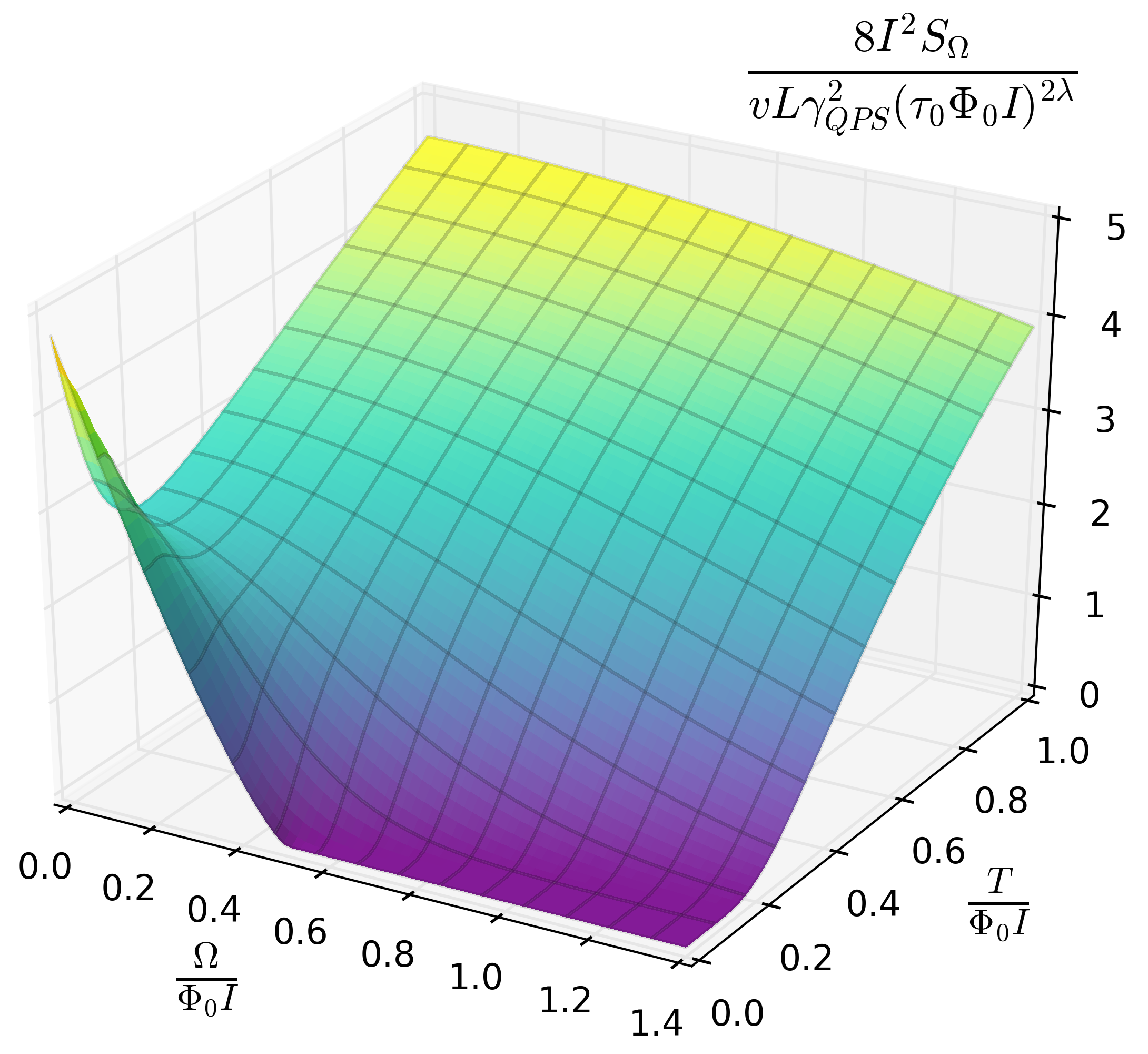
Figure 2: The dependence of QPS noise power $S_{\Omega}$ (29) at $\lambda=2.3$ from frequency $\Omega$ and temperature $T$.

At $T\to 0$ from Eq. (29) we find

$$S_{\Omega}^{QPS}\propto\begin{cases}I^{\lambda-1}(I-2\Omega/\Phi_{0})^{\lambda-1},&\Omega<\Phi_{0}I/2,\\ 0,&\Omega>\Phi_{0}I/2.\end{cases}$$ (31)

In order to interpret this threshold behaviour let us bear in mind that at $T=0$ each QPS event can excite 2$N$ plasmons ($N=1,2...$) with total energy $E=\Phi_{0}I$ and total zero momentum. The left and the right moving plasmons (each group carrying total energy $E/2$) eventually reach respectively the left and the right voltage probes which then detect voltage fluctuations with frequency $\Omega$. As in the long wire limit and for non-zero $\Omega$ these two groups of plasmons become totally uncorrelated, it is obvious that at $T=0$ voltage noise can only be detected at $\Omega<E/2$ in the agreement with Eq. (31).

In summary, we investigated QPS-induced voltage fluctuations in superconducting nanowires within the four-point measurement scheme. We demonstrated that shot noise detected in such nanowires may essentially depend on the particular measurement setup. In long wires and at non-zero frequencies quantum voltage noise is essentially determined by plasmons created by QPS events and propagating in opposite directions along the wire. As a result, at $T\to 0$ the shot noise vanishes at frequencies exceeding $\Phi_{0}I/2$.

This work was supported in part by RFBR grant No. 15-02-08273. It has been presented at the International Conference SUPERSTRIPES 2016 superstr20016 .

References

• (1) K.Yu. Arutyunov, D.S. Golubev, and A.D. Zaikin, Superonductivity in one dimension, Phys. Rep. 464, 1 (2008).
• (2) A.D. Zaikin et al., Quantum phase slips and transport in ultrathin superconducting wires, Phys. Rev. Lett. 78, 1552 (1997).
• (3) D.S. Golubev and A.D. Zaikin, Quantum tunneling of the order parameter in superconducting nanowires, Phys. Rev. B 64, 014504 (2001).
• (4) A. Bezryadin, C.N. Lau, and M. Tinkham, Quantum suppression of superconductivity in ultrathin nanowires, Nature 404, 971 (2000).
• (5) C.N. Lau et al., Quantum phase slips in superconducting nanowires, Phys. Rev. Lett. 87, 217003 (2001).
• (6) M. Zgirski et al., Quantum fluctuations in ultranarrow supercooducting aluminum nanowires, Phys. Rev. B 77, 054508 (2008).
• (7) X.D.A. Baumans et al., Thermal and quantum depletion of supercondutivity in narrow junctions created by controlled electromigration, Nat. Commun. 7, 10560 (2016).
• (8) A.G. Semenov and A.D. Zaikin, Quantum phase slip noise, Phys. Rev. B 94, 014512 (2016).
• (9) A.G. Semenov and A.D. Zaikin, Quantum phase slips and voltage fluctuations in superconducting nanowires, Fortschr. Phys. 64, XXX (2016).
• (10) A.G. Semenov and A.D. Zaikin, Persistent currents in quantum phase slip rings, Phys. Rev. B 88, 054505 (2013).
• (11) J.E. Mooij and G. Schön, Propagating plasma mode in thin superconducting filaments, Phys. Rev. Lett. 55, 114 (1985).
• (12) T. Adachi et al. Superstripes 2016 (Superstripes Press, Rome, Italy) ISBN 9788866830559.