Dual cascade and dissipation mechanisms in helical quantum turbulence

Abstract

While in classical turbulence helicity depletes nonlinearity and can alter the evolution of turbulent flows, in quantum turbulence its role is not fully understood. We present numerical simulations of the free decay of a helical quantum turbulent flow using the Gross-Pitaevskii equation at high spatial resolution. The evolution has remarkable similarities with classical flows, which go as far as displaying a dual transfer of incompressible kinetic energy and helicity to small scales. Spatio-temporal analysis indicates that both quantities are dissipated at small scales through non-linear excitation of Kelvin waves and the subsequent emission of phonons. At the onset of the decay, the resulting turbulent flow displays polarized large scale structures and unpolarized patches of quiescense reminiscent of those observed in simulations of classical turbulence at very large Reynolds numbers.

I Introduction

From the oceans to the solar wind, turbulence is widely found in nature. It is also observed in quantum fluids such as superfluids and Bose-Einstein condensates (BECs) Barenghi et al. (2014). Unlike classical flows, quantum flows have no viscosity and vorticity is concentrated along topological line defects with quantized circulation Feynman (1955); Donnelly (1991). While similarities between these two types of turbulence exist (e.g., both display Kolmogorov spectrum Maurer and Tabeling (1998); Salort et al. (2012)), there are also differences Paoletti et al. (2008); White et al. (2010).

In classical turbulence helicity is an ideal invariant which measures how tangled vorticity field lines are Moffatt (1969). It is known to deplete nonlinearities and energy transfer (Kraichnan, 1973), slow down the onset of dissipation in decaying turbulence and affect its dissipation scale (André and Lesieur, 1977), play a role in convective storms (Lilly, 1986), and display a dual direct cascade with the energy Brissaud et al. (1973); Moffatt and Tsinober (1992). Its role in quantum turbulence is less clear. Efforts focus on determining if it is conserved by studying simple configurations of reconnecting vortex knots Scheeler et al. (2014); Zuccher and Ricca (2015); Kleckner et al. (2016); Clark di Leoni et al. (2016); Hänninen et al. (2016). Numerical evidence indicates that in this case helicity is transferred from large to small scales Scheeler et al. (2014); Kleckner et al. (2016), and that reconnection or the transfer of helicity can excite non-linear interacting Kelvin waves Fonda et al. (2014); Clark di Leoni et al. (2016), which eventually may lead to a loss of helicity by sound emission. Research into the role of helicity in more complex quantum flows has been lacking, partly due to the difficulties of quantifying helicity in fully developed turbulent flows. However, new developments in 3D vortex tracking in Helium experiments Lathrop and in knot generation in BECs Hall et al. (2016) provide hopeful opportunities to tackle this problem.

We present massive numerical simulations of helical quantum turbulence using the Gross-Pitaevskii equation (GPE) as a model. A quantum version of the classical Arnold-Beltrami-Childress (ABC) flow is introduced and used as initial condition to create a helical flow. We use different methods to quantify helicity, including the regularized helicity Clark di Leoni et al. (2016) which was shown to give results equivalent to the centerline helicity for simple knots, and to the classical helicity for flows with scale separation. We show that helicity is depleted as the incompressible kinetic energy. As in the classical case Brissaud et al. (1973), both the incompressible energy and the helicity follow a Kolmogorov spectrum down to the intervortex distance. At smaller scales a bottleneck in the energy spectrum is followed by another Kolmogorov spectrum associated to a Kelvin waves cascade. Energy and helicity dissipation at coherent length scales is related to Kelvin waves damping by phonon emision. In physical space, the flow displays polarized large scale structures formed by a myriad of small scale knots, and unpolarized quiescent patches mimicking what is observed in isotropic and homogeneous classical flows at large Reynolds. These results open up new questions about helicity in quantum flows. In particular, while successful theories for the energy spectrum exist (L’vov and Nazarenko, 2010), this is not yet the case for the helicity spectrum.

II The Gross-Pitaevskii equation

The GPE describes the evolution of a zero-temperature condensate of weakly interacting bosons of mass $m$,

$$i\hbar\partial_{t}\Psi=-\hbar^{2}(2m)^{-1}\nabla^{2}\Psi+g|\Psi|^{2}\Psi,$$ (1)

where $g$ is related to the scattering length. Madelung transformation $\Psi=\sqrt{{\rho}/{m}}\exp{(im\phi/\hbar)}$ relates the wavefunction $\Psi$ to a condensate of density $\rho$ and velocity ${\bf v}={\bf\nabla}\phi$. Linearizing Eq. (1) around a constant $\Psi=\hat{\Psi}_{\bf 0}$ yields the Bogoliubov dispersion relation $\omega_{B}(k)=ck(1+\xi^{2}k^{2}/2)^{1/2}$ for sound waves (or phonons) of speed $c=(g|\hat{\Psi}_{\bf 0}|^{2}/m)^{1/2}$, with dispersion taking place at lengths smaller than the coherence length $\xi=[g\hbar^{2}|\hat{\Psi}_{\bf 0}|^{2}/(2m)]^{1/2}$. The Onsager-Feynman quantum of velocity circulation around the $\Psi=0$ topological defect lines is $h/m$, and the vortex core size is of order $\xi$ Proukakis and Jackson (2008).

The GPE conserves the total energy $E$, which can be decomposed as Nore et al. (1997a, b):

$$E=E_{\rm kin}+E_{\rm int}+E_{\rm q},$$ (2)

with the kinetic energy $E_{\rm kin}=\langle|\sqrt{\rho}{\bf v}|^{2}/2\rangle$, the internal energy $E_{\rm int}=\langle c^{2}(\rho-1)^{2}/2\rangle$ and the so-called quantum energy $E_{\rm q}=\langle c^{2}\xi^{2}|\nabla\sqrt{\rho}|^{2}\rangle$. The kinetic energy $E_{\rm kin}$ can be also decomposed into compressible $E_{\rm kin}^{\rm c}$ and incompressible $E_{\rm kin}^{\rm i}$ components, using $(\sqrt{\rho}{\bf v})=(\sqrt{\rho}{\bf v})^{\rm c}+(\sqrt{\rho}{\bf v})^{\rm i}$ with $\nabla\cdot(\sqrt{\rho}{\bf v})^{\rm i}=0$.

II.1 Helicity in quantum flows

The definition of helicity in a classical flow is

$$H=\int{\bf v}\cdot{\bm{\omega}}\,dV,$$ (3)

where ${\bm{\omega}}=\nabla\times{\bf v}$ is the vorticity. It follows from Madelung transformation that

$${\bm{\omega}}({\bf r})=\frac{h}{m}\int ds\frac{d{\bf r}_{0}}{ds}\delta({\bf r}-{\bf r}_{0}(s)),$$ (4)

where ${\bf r}_{0}(s)$ denotes the position of the vortex lines and $s$ the arclength. Thus vorticity in a quantum flow is a distribution concentrated along $\Psi=0$ topological line defects where ${\bf v}$ is ill-behaved. In spite of this, some authors Zuccher and Ricca (2015) compute $H$ by filtering fields to the largest scales or relying on the regularization introduced by the numerics. Other authors compute the “centerline helicity” by calculating the writhe and link, two topological quantities which quantify how knotted vortex lines are, but which require detailed extraction of all centerlines of the quantized vortices in the flow Scheeler et al. (2014); Laing et al. (2015); Kleckner et al. (2016); Villois et al. (2016). Some authors suggest to also add the twist of equal-phase surfaces (or else just the torsion) to this definition, but then the total helicity vanishes identically (or else smoothly formed inflection points change the helicity discontinuously) Hänninen et al. (2016). A new method which yields the same results as the “centerline helicity” was introduced in Clark di Leoni et al. (2016) by using the fact that the velocity parallel to the quantized vortex has only an apparent singularity. The regular smooth velocity oriented along the vortex line is defined as ${\bf v}_{\rm reg}={v_{\parallel}{\bf w}}/{\sqrt{{w}_{j}{w}_{j}}}$, where

$$v_{\parallel}=\frac{\hbar\,{w}_{j}\left[(\partial_{j}\partial_{l}\Psi)\partial_{l}\overline{\Psi}-(\partial_{j}\partial_{l}\overline{\Psi})\partial_{l}\Psi\right]}{2im\sqrt{{w}_{l}{w}_{l}}(\partial_{m}\Psi)(\partial_{m}\overline{\Psi})},$$ (5)

and

$${\bf w}=\frac{\hbar}{im}\bm{\nabla}\overline{\Psi}\times\bm{\nabla}\Psi$$ (6)

(see Appendix A for a detailed derivation). The regularized helicity thus reads

$$H_{r}=\int{\bf v}_{\rm reg}\cdot{\bm{\omega}}\,dV,$$ (7)

and is well defined in the sense of distributions Lighthill (1958), as the test function ${\bf v}_{\rm reg}$ is smooth. This expression was proven useful even in flows with hundreds of thousands of knots.

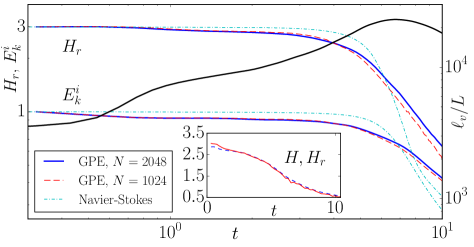
Figure 1: (Color online) Evolution of the incompressible energy $E^{i}_{k}$ and of the regularized helicity $H_{r}$ in the $1024^{3}$ and $2048^{3}$ GPE runs, and in Navier-Stokes. Note the early “inviscid” phase in which quantities are approximately constant. The solid black line shows the total vortex length in the $2048^{3}$ GPE run. Inset: $H_{r}(t)$ (dashed blue line) and the non regularized helicity $H(t)$ (solid red line) in the $2048^{3}$ GPE run.

II.2 Numerical simulations

The GPE is solved in its dimensionless form and all quantities presented here are dimnesionless (see Nore et al. (1997b); Clark di Leoni et al. (2015) for more details). All numerical simulations in this paper have mean density $\rho_{0}=1$. Physical constants in Eq. (1) are determined by $\xi$ and $c=2$, and the quantum of circulation $h/m=c\xi/\sqrt{2}$. Simulations were performed using $512^{3}$, $1024^{3}$, and $2048^{3}$ grid points, in a domain of linear size $L=2\pi$. The largest $2048^{3}$ GPE simulation has a healing length $\xi\approx 2.2\times 10^{-3}$ and an intervortex distance $\ell\approx 8\times 10^{-2}$ (computed as in Nore et al. (1997a, b)). As a comparison, in ${}^{3}He$ experiments the size of the vortex core is $\approx 10^{-8}$ m, the intervortex distance is $\approx 10^{-5}$ m, and the system size is of order $10^{-2}$ m Barenghi et al. (2014). Scale separation is smaller for BECs, which are also better modeled by the GPE. Although proper scale separation in a simulation is currently out of reach, the $2048^{3}$ run is a significant improvement over most simulations of quantum turbulence which have one order or magnitude difference between $L$ and $\xi$.

Figure 2: (Color online) Spectrum of the (a) incompressible kinetic energy, and (b) helicity in the $2048^{3}$ GPE run. At large scales both follow a scaling compatible with a classical dual cascade (thick dashed lines). At scales smaller than the intervortex scale ($k_{\ell}\approx 80$) a second range compatible with a Kelvin wave cascade is observed in $E^{i}_{k}$ (thick dash-dotted line). The helicity spectrum broadens in time indicating a direct transfer.

Figure 3: (Color online) Compensated helicity spectra in the $2048^{3}$ GPE run. The spectrum is compatible with $\eta\epsilon^{-1/3}k^{-5/3}$ scaling. The time-averaged spectrum is also shown.

To compare the GPE simulations with classical ABC flows we also simulated the incompressible Navier-Stokes (NS) equation

$$\partial_{t}\bf{u}+({\bf u}\cdot\nabla){\bf u}=-\nabla p+\nu\nabla^{2}{\bf u},$$ (8)

with $\nabla\cdot\bf{u}=0$, using $512^{3}$ points and viscosity $\nu=6.5\times 10^{-4}$. All equations were integrated using GHOST Mininni et al. (2011), a pseudospectral code with periodic boundary conditions, fourth order Runge-Kutta to compute time derivatives, and the $2/3$ rule for dealiasing.

As initial condition we use a superposition of $k=1$ and $k=2$ basic ABC flows: ${\bf v}_{\rm ABC}={\bf v}_{\rm ABC}^{(1)}+{\bf v}_{\rm ABC}^{(2)}$, with

$${\bf v}_{\rm ABC}^{(k)}= \left[B\cos(ky)+C\sin(kz)\right]\hat{x}+\left[C\cos(kz)+\right.$$ (9)

$$\left.A\sin(kx)\right]\hat{y}+\left[A\cos(kx)+B\sin(ky)\right]\hat{z},$$

and $(A,B,C)=(0.9,1,1.1)/\sqrt{3}$. The basic ABC flow is a $2\pi$-periodic stationary solution of the Euler equation with maximal helicity. To build its quantum version we first take the flow with $B=C=0$ and use Madelung transformation to obtain a wavefunction $\Psi_{A,k}^{x,y,z}=\exp\{i[A\sin(kx)\,m/\hbar]y+i[A\cos(kx)\,m/\hbar]z\}$, where $[a]$ stands for the nearest integer to $a$ to enforce periodicity. The wavefunction of the quantum ABC flow is then obtained as $\Psi_{\rm ABC}^{(k)}=\Psi_{A,k}^{x,y,z}\times\Psi_{B,k}^{y,z,x}\times\Psi_{C,k}^{z,x,y}$. Finally, $\Psi_{\rm ABC}=\Psi_{\rm ABC}^{(1)}\times\Psi_{\rm ABC}^{(2)}$ corresponds to the initial flow ${\bf v}_{\rm ABC}$. In practice, to correctly set the initial density with defects along the vortex lines and to correct frustration errors arising from periodicity, following Nore et al. (1997a, b) we first evolve $\Psi_{\rm ABC}$ using the advected real Guinzburg-Landau equation , whose stationary solutions are solutions of the GPE with minimal emission of acoustic energy.

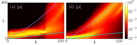
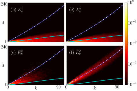
Figure 4: (Color online) Spatio-temporal power spectra for the $512^{3}$ GPE run between $t=0$ and $2$ for (a) the mass density $\rho$, and zooms between $k=0$ and $100$ for (b) the incompressible and (c) compressible velocity. Same for late times ($t\in[8,10]$) are shown in (d), (e), and (f). The solid (green) curve is the dispersion relation of Kelvin waves, while the dotted (white) curve corresponds to sound waves.

III Results

In Fig. 1 we show the evolution of the incompressible kinetic energy $E^{i}_{k}$ and of the regularized helicity $H_{r}$ for the $1024^{3}$ and $2048^{3}$ GPE runs, and for the NS equation (with $H_{r}\equiv H$). In all cases, $E^{i}_{k}$ and $H_{r}$ remain approximately constant for the first turnover times while turbulence develops (the so-called “inviscid” phase in the decay of classical flows). The total vortex length $\ell_{v}$ peaks at the end of this phase, which ends slightly earlier for $H_{r}$ than for $E^{i}_{k}$. Afterwards, $H_{r}$ and $E^{i}_{k}$ decrease in what seems a self-similar decay, with different rates in each system. As total energy is conserved in GPE, the decay of $E^{i}_{k}$ is accompanied by a growth of the other components of the energy, in particular of $E^{c}_{k}$. Indeed, in quantum turbulence the decay of $E^{i}_{k}$ is expected to result from the emission of phonons Vinen and Niemela (2002), and thus from classical results Teitelbaum and Mininni (2011) the decay in $E^{i}_{k}$ should also produce a decay in $H_{r}$.

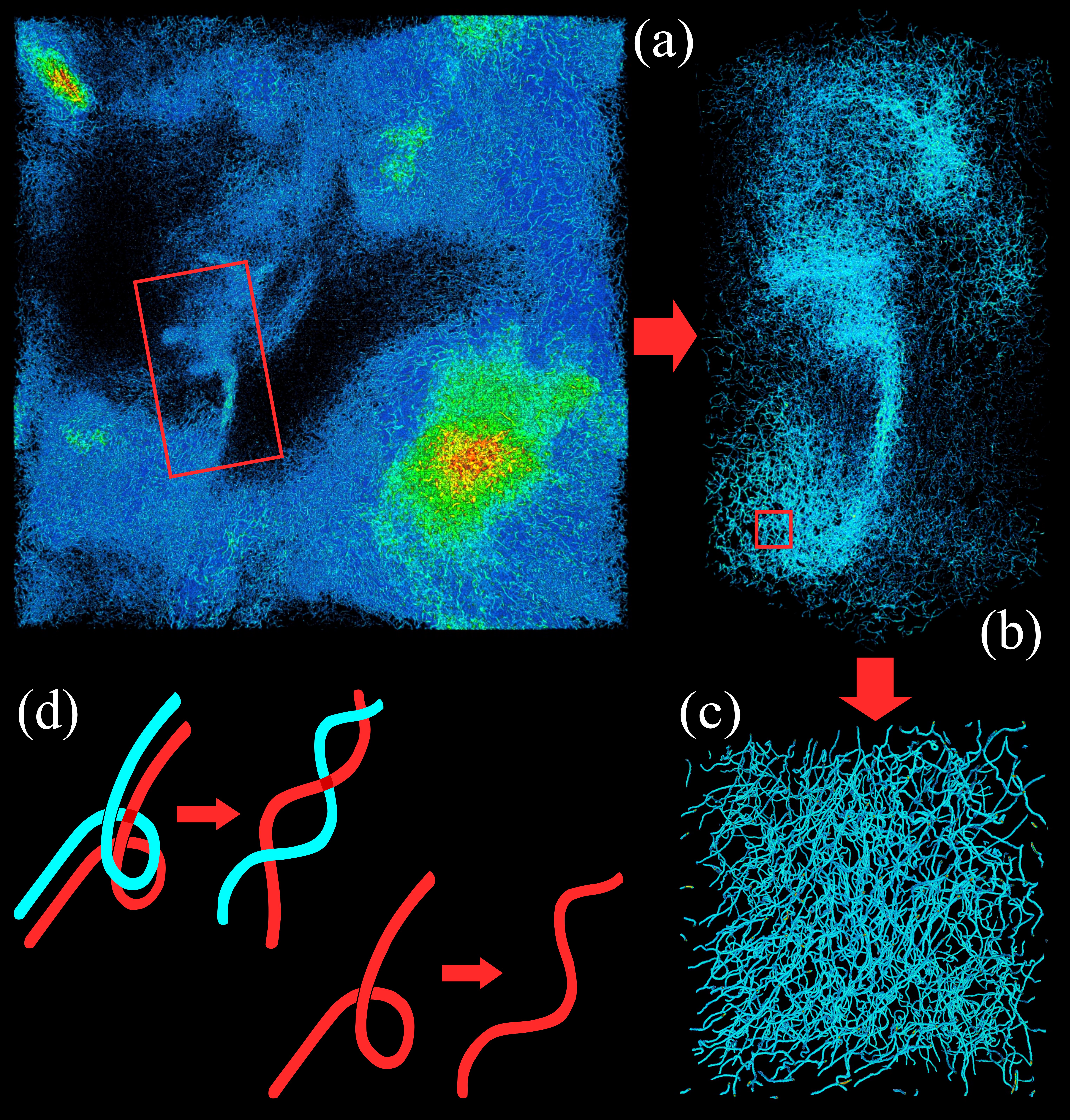
Figure 5: (Color online) Three-dimensional rendering of vortex lines at the onset of the decay in the $2048^{4}$ GPE run of (a) a slice of the full box, and succesive zooms in (b) and (c) into the regions indicated by the (red) rectangles. (d) Sketch of the transfer of helicity from writhe to twist in a bundle of vortices, and for an individual vortex.

The inset in Fig. 1 compares $H$ (non regularized) and $H_{r}$ in the $2048^{3}$ GPE run. Both are in good agreement, but $H_{r}$ is smoother and less noisy, making it a better fit to study the global evolution of helicity in quantum turbulence. However, the agreement between $H_{r}$ and $H$ allows us to use $H$ to compute spectra.

Figure 2 shows spectra of $E^{i}_{k}$ and $H$ at different times in the $2048^{3}$ GPE run. The spectra build up rapidly from the initial conditions, and the energy and helicity excite larger wavenumbers as time increases. At $t=5$ both already display inertial ranges. At large scales they follow a power law compatible with a classical dual energy and helicity cascade Brissaud et al. (1973), with Kolmogorov constant $C_{K}\approx 1$

$$E(k)\approx\epsilon^{2/3}k^{-5/3},\hskip 14.22636ptH(k)\approx\eta\epsilon^{-1/3}k^{-5/3},$$ (10)

and with $\epsilon$ and $\eta$ calculated directly using

$$\epsilon=-dE^{i}_{k}/dt,\,\,\,\,\eta=-dH/dt,$$ (11)

from the data in Fig. 1 after the onset of decay. Around the mean intervortex scale ($k_{\ell}\approx 80$) $E^{i}_{k}$ diplays a bottleneck compatible with predictions in L’vov and Nazarenko (2010). This bottleneck is followed by an inertial range $\sim k^{-5/3}$ predicted for a Kelvin wave cascade L’vov and Nazarenko (2010); Krstulovic (2012) and which below is confirmed for the lower resolution run. Figure 3 shows compensated helicity spectra, which corroborates the behavior observed in Fig. 2.

Of particular interest is the evolution of $H(k)$. For early times $H$ is concentrated at low wavenumbers, as expected for the initial condition. But later it is transferred to larger wavenumbers as the cascade-like spectrum develops. While there is no rigourous proof of conservation of helicity in quantum flows, note that using the Hasimoto transformation Hasimoto (1972) the evolution of a vortex line can be mapped into a nonlinear Schrödinger equation which conserves momentum. But momentum of a vortex line (e.g., the translation of the centerline in the direction of vorticity) can result in net helicity. Thus, vortex lines evolution could indeed conserve helicity (except for depletion by emission of phonons). At small scales $H(k)$ displays wild fluctuations (in amplitude and sign), which is to be expected as the non-reguralized helicity is ill-behaved at those scales. The fact that the helicity dynamics, at least at large scales, of a quantum flow mimics those of a classical one is remarkable. But it also begs the question of what happens to the helicity at scales smaller than the intervortex distance. Indications exist that Kelvin waves carry helicity Scheeler et al. (2014); Clark di Leoni et al. (2016), but such a possibility requires confirmation of their presence.

Figure 6: (Color online) Correlation function of $\rho$ in the $2048^{3}$ GPE run. At $t=0$ it decays rapidly in units of the healing length $\xi$, but then quickly develops long-range correlations. Inset: Ratio of eigenvalues $\lambda_{max}/\lambda_{min}$ as a function of $2\pi/d$, with $d$ the size of the box used for the average (blue triangles: regions with structures, red triangles: regions of quiescence).

To verify this, as well as phonons being the dissipation mechanism for $E^{i}_{k}$ and $H$, we must detect Kelvin and sound waves. To do this we use the spatio-temporal spectrum Clark di Leoni et al. (2015), i.e., the four-dimensional power spectrum of a field as a function of wave vector and frequency. The spectrum allows quantification of how much power is in each mode $({\bf k},\omega)$, and waves can be separated from the rest as they satisfy a known dispersion relation $\omega({\bf k})$. As its computation requires huge amounts of data (i.e., storage of fields resolved in space and time), we compute it for the $512^{3}$ GPE run. Figure 4 shows this spectrum (after integration in ${\bf k}$ using isotropy to obtain dependency on $k$ and $\omega$) for $\rho$, and zooms for small $k$ for $E^{i}_{k}$ and $E^{c}_{k}$, for early and late times (respectively, $t\in[0,2]$ and $t\in[8,10]$). The dispersion relation of Kelvin $\omega_{K}(k)$ and sound waves $\omega_{B}(k)$ are shown. Note that, compared with the $2048^{3}$ run, $\xi$ in this run is 4 times larger, and values of $k$ are 4 times smaller.

At early times, power in the spatio-temporal spectrum of $\rho$ is broadly spread over modes that do not correspond to waves. $E^{i}_{k}$ shows some excitations compatible with Kelvin waves, and $E^{c}_{k}$ has little energy with no phonon excitation. At late times power in fluctuations of $\rho$ moves towards the Kelvin wave dispersion relation up to $k\approx 80$, and then the power jumps towards the dispersion relation of phonons. The spectra $E^{i}_{k}$ and $E^{c}_{k}$ confirm this picture, with power concentrating in $E^{c}_{k}$ in the vicinity of the sound dispersion relation. Exploration of these spectra for different time ranges shows that as time evolves more energy goes from Kelvin wave modes to phonons. While this analysis is performed at lower resolution and thus wavenumbers for the transition are smaller than in the $2048^{3}$ run, the spectra confirm the dynamics in Figs. 1 and 4: with time, energy and helicity go from large to smaller scales in which Kelvin waves are excited, and they are finally dissipated into phonons.

This can be further confirmed by visualizing vortices in real space at the onset of decay. Figure 5 shows a three-dimensional rendering of quantum vortices at $t\approx 2.5$ in the $2048^{3}$ GPE run. Large-scale eddies, formed up by a myriad of small-scale and knotted vortices, emerge. Similar behavior has been observed at finite temperature quantum turbulence simulations, where the bundle was correlated with high vorticity in the normal fluid component Morris et al. (2008); Nemirovskii (2013). At zero temperature two results Sasa et al. (2011); Baggaley et al. (2012a, b) also hinted at this behavior, but in none the fine structure of the vortex bundle was resolved. More importantly, the large scale flow shows inhomogeneous regions with high density of vortices and quiet regions with low density. These large-scale patches were not present in the initial conditions (which have homogeneously distributed vortices) and are created by the evolution as shown below. The patches are reminiscent of those observed in isotropic and homogeneous turbulence at high resolution in non-helical Ishihara et al. (2009) and helical Mininni et al. (2006) flows, further confirming the similarity between quantum and classical turbulence at scales larger than the intervortex separation.

The spontaneous emergence of large-scale correlations in the system can be confirmed by the spatial correlation function

$$C(d)=\left<(\rho({\bf x}+d\hat{x})-\rho_{0})(\rho({\bf x})-\rho_{0})\right>,$$ (12)

shown in Fig. 6. This correlation function is related to the internal energy spectrum by the Wiener-Khinchin theorem. At $t=0$, $C(d)$ decays rapidly in units of the healing length $\xi$, and it is dominated by the vortex core size. But the system rapidly develops long-range correlations (up to $\approx 1000\xi$) and later $C$ decays in a self-similar way. Furthermore, computing the ratio of eigenvalues $\tau=\lambda_{max}/\lambda_{min}$ for the tensor $\langle\partial_{i}\rho\partial_{j}\rho\rangle$ averaged in boxes of size $1/10$ of the linear domain size, typically yields $\tau\approx 3$ in regions with large scale structures and $\tau\approx 1$ in quiescent regions, indicating anisotropy and a copious vortex polarization in the former (see Fig. 6 inset).

IV Conclusions

The results indicate that helicity can be conserved in quantum turbulence at large-scales and as it is transferred towards smaller scales (see Fig. 2), but eventually it decays through the emission of phonons produced by a Kelvin wave cascade (Fig. 4). We can draw a comparison with the classical case, where now a bundle of quantum vortices (as seen in Fig. 5) would play the role of classical vortex tubes. Tubes, in contrast to lines, add an extra degree of freedom to the helicity: their twist. Thus in the classical and quantum cases, large scale helicity can be transformed from writhe to twist for a bundle of vortices (see Fig. 5.d). But for individual quantum vortices, the transfer (e.g., through reconnection) would result in the excitation of a Kelvin wave which can eventually be damped. This indicates that individual quantum vortex lines behave like classical vortex tubes with a mechanism to relax the twist, and as such, the correct analogy between classical and quantum flows only holds for scales larger than $\ell$ for which bundles of quantum vortices behave as classical vortex tubes.

Appendix A Derivation of the regularized velocity

To calculate the helicity in a quantum flow we need information of both the velocity and the vorticity along the vortex lines. This is problematic as both quantities have singularities along those lines. Therefore, we need to regularize one of them in order to have a well-behaved integral for the helicity (in the sense of distributions Lighthill (1958)). Although in principle it may seem possible to regularize any of the two fields, the choice of regularizing the velocity and not the vorticity is not arbitrary. In the Gross-Pitaevskii equation, the vorticity is correctly described by a distribution. Instead, the only component of the velocity that is not well behaved is the one perpendicular to the vortex line. But for the calculation of the helicity we need the parallel component, whose problem is to have a $0/0$ indeterminacy in its defintion. Thus, regularizing the velocity allows us to keep its well defined component which contributes to the helicity, while leaving the vorticity as a Dirac delta distribution also allows us to not bother with the values of the regularized field outside the vortex line, which should give no contribution to the helicity. Here we outline a detailed explanation of how to derive the regularized velocity, from which the expression of the regularized helicity follows immediately.

The velocity of the superfluid is given by

$${\bf v}=\frac{\hbar}{2im}\frac{\bar{\Psi}\bm{\nabla}\Psi-\Psi\bm{\nabla}\bar{\Psi}}{\Psi\bar{\Psi}}.$$ (13)

Without loss of generality we can suppose that there is a vortex line going through ${\bf r}=0$ (the radial cylindrical vector) in the direction of the $z$-axis. Let us define the unit vector basis $({\bf\hat{e}}_{x},{\bf\hat{e}}_{y},{\bf\hat{e}}_{z})$. The existence of a vortex line passing through $\bf{r}=0$ and pointing in the $z$-direction implies that $\Psi(0)=0$, $\bar{\Psi}(0)=0$, ${\bf\hat{e}}_{z}\cdot\bm{\nabla}\Psi(0)=0$, and ${\bf\hat{e}}_{z}\cdot\bm{\nabla}\bar{\Psi}(0)=0$. Thus $\bm{\nabla}\Psi(0)$ and $\bm{\nabla}\bar{\Psi}(0)$ are linear combinations of ${\bf\hat{e}}_{x}$ and ${\bf\hat{e}}_{y}$. Taylor-expanding to first order the numerator and denominator of the above expression for ${\bf v}({\bf r})$ around ${\bf r}=0$ one finds

$$\Psi(x,y,z) =x\partial_{x}\Psi(0)+y\partial_{y}\Psi(0)+\mathcal{O}({\bf r}^{2}),$$ (14)

$$\bar{\Psi}(x,y,z) =x\partial_{x}\bar{\Psi}(0)+y\partial_{y}\bar{\Psi}(0)+\mathcal{O}({\bf r}^{2}),$$ (15)

$$\bm{\nabla}\Psi(x,y,z) =\bm{\nabla}\Psi(0)+{\bf r}\cdot\bm{\nabla}(\bm{\nabla}\Psi)(0)+\mathcal{O}({\bf r}^{2}),$$ (16)

$$\bm{\nabla}\bar{\Psi}(x,y,z) =\bm{\nabla}\bar{\Psi}(0)+{\bf r}\cdot\bm{\nabla}(\bm{\nabla}\bar{\Psi})(0)+\mathcal{O}({\bf r}^{2}).$$ (17)

After replacing the above expressions in Eq. (13) and dropping quadratic terms, the perpendicular ($x$ and $y$) components of the velocity diverge in the limit ${\bf r}\to 0$, as ${\bf v}_{\perp}$ reads

$${\bf v}_{\perp}({\bf r})=\frac{\hbar}{2im}\left(\frac{\nabla\Psi(0)}{x\partial_{x}\Psi(0)+y\partial_{y}\Psi(0)}-c.c\right).$$ (18)

On the other hand, the velocity component parallel to the centerline vorticity $v_{\parallel}({\bf r})={\bf v}({\bf r})\cdot{\bf\hat{e}}_{z}$ reads

$$v_{\parallel}({\bf r})=\frac{\hbar}{2im} \left(\frac{x(\partial_{xz}\Psi)(0)+y(\partial_{yz}\Psi)(0)+z(\partial_{zz}\Psi)(0)}{x\partial_{x}\Psi(0)+y\partial_{y}\Psi(0)}\right.$$

$$\left.-c.c.\vphantom{\frac{1}{2}}\right),$$ (19)

which is finite in the limit ${\bf r}\to 0$. This last expression for $v_{\parallel}(\bf r)$ can be seen as resulting from l’Hôpital’s rule applied to the limit of $v_{\parallel}{(\bf r})$ when ${\bf r}\to 0$ in the direction $(x,y,z)$. The limit obviously depends on the direction as, in deriving the above formulae, the only hypotheses we have made are that $\Psi$ is sufficiently differentiable and has a zero-line directed toward $z$.

In order to turn the above expression into a workable ansatz for $v_{\parallel}(0)$, we need to pick a reasonable direction along which $\Psi$ will have a significant variation. The simplest vectors we have at point ${\bf r}=0$, perpendicular to the vortex line and satisfying the condition, are $\bm{\nabla}\Psi(0)$ and $\bm{\nabla}\bar{\Psi}(0)$. Thus we can multiply the first term in the r.h.s. of Eq. (19) by $\bm{\nabla}\bar{\Psi}$, and its complex conjugate by $\bm{\nabla}\Psi$ in order to maintain the reality of the velocity field. In this way we arrive to the following expression

$$v_{\parallel}(0)=\frac{\hbar}{2m\,i}(\frac{\partial_{x}\bar{\Psi}\partial_{xz}\Psi+\partial_{y}\bar{\Psi}\partial_{yz}\Psi+\partial_{z}\bar{\Psi}\partial_{zz}\Psi}{\partial_{x}\bar{\Psi}\partial_{x}\Psi+\partial_{y}\bar{\Psi}\partial_{y}\Psi+\partial_{z}\bar{\Psi}\partial_{z}\Psi}-c.c.).$$ (20)

A first check that this ansatz is reasonable is to plug in $\Psi\sim(x+iy)e^{izU_{z}m/\hbar}$ and explicitly verify that this gives $v_{\parallel}(0)=U_{z}$. Further validations were performed in Clark di Leoni et al. (2016), where it was shown that the helicity computed with the regularized velocity agrees with the topological definitions of writhe, link, and twist. Also, in Clark di Leoni et al. (2016) it was shown that this expression gives the correct value of helicity for different knots, and that in quantum flows with helicity it gives a value that matches the helicity in the equivalent classical large-scale helical flow.

As a final remark, it is important to note that for arbitrarily aligned vortex lines, the direction parallel to the vortex line ($\hat{z}$ in the particular case considered above) can be easily obtained by doing the vector product between $\bm{\nabla}\Psi$ and $\bm{\nabla}\bar{\Psi}$.