Policy Iterations for Reinforcement Learning Problems in Continuous Time and Space — Fundamental Theory and Methods

Abstract

Policy iteration (PI) is a recursive process of policy evaluation and improvement for solving an optimal decision-making/control problem, or in other words, a reinforcement learning (RL) problem. PI has also served as the fundamental for developing RL methods. In this paper, we propose two PI methods, called differential PI (DPI) and integral PI (IPI), and their variants, for a general RL framework in continuous time and space (CTS), where the environment is modeled by a system of ordinary differential equations (ODEs). The proposed methods inherit the current ideas of PI in classical RL and optimal control and theoretically support the existing RL algorithms in CTS: TD-learning and value-gradient-based (VGB) greedy policy update. We also provide case studies including 1) discounted RL and 2) optimal control tasks. Fundamental mathematical properties — admissibility, uniqueness of the solution to the Bellman equation (BE), monotone improvement, convergence, and optimality of the solution to the Hamilton-Jacobi-Bellman equation (HJBE) — are all investigated in-depth and improved from the existing theory, along with the general and case studies. Finally, the proposed ones are simulated with an inverted-pendulum model and their model-based and partially model-free implementations to support the theory and further investigate them beyond.

, [JYLee]Corresponding author. Tel.: +1 587 597 8677.

1 Introduction

Policy iteration (PI) is a class of approximate dynamic programming (ADP) for recursively solving an optimal decision-making/control problem by alternating between policy evaluation to obtain the value function (VF) w.r.t. the current policy (a.k.a. the current control law in control theory) and policy improvement to improve the policy by optimizing it using the obtained VF (Sutton and Barto, 2018; Puterman, 1994; Lewis and Vrabie, 2009). PI was first proposed by Howard (1960) in a stochastic environment known as the Markov decision process (MDP) and has served as a fundamental principle for developing RL methods, especially for an environment modeled or approximated by an MDP in discrete time and space. Convergence of such PIs towards the optimal solution has been proven, with the finite-time convergence for a finite MDP (Puterman, 1994, Theorems 6.4.2 and 6.4.6); the forward-in-time computation of PI like the other ADP methods alleviates the problem known as the curse of dimensionality (Powell, 2007). A discount factor $\gamma\in[0,1]$ is normally introduced to both PI and RL to suppress the future reward and thereby have a finite return. Sutton and Barto (2018) give a comprehensive overview of PI and RL algorithms with their practical applications and recent success.

On the other hand, the dynamics of a real physical task is in the majority of cases modeled as a system of (ordinary) differential equations (ODEs) inevitably in continuous time and space (CTS). PI has also been studied in such a continuous domain mainly under the framework of deterministic optimal control, where the optimal solution is characterized by the partial differential Hamilton-Jacobi-Bellman (HJB) equation (HJBE). However, an HJBE is extremely difficult or hopeless to solve analytically, except for a very few exceptional cases. PI methods in this field are often referred to as successive approximations of the HJBE (for recursively solving it!), and the main difference among them lies in their policy evaluation — the earlier PI methods solve the associated differential Bellman equation (BE) (a.k.a. Lyapunov or Hamiltonian equation) to obtain each VF for the target policy (e.g., Leake and Liu, 1967; Kleinman, 1968; Saridis and Lee, 1979; Beard, Saridis, and Wen, 1997; Abu-Khalaf and Lewis, 2005 to name a few). Murray, Cox, Lendaris, and Saeks (2002) proposed a trajectory-based policy evaluation that can be viewed as a deterministic Monte-Carlo prediction (Sutton and Barto, 2018). Motivated by those two approaches above, Vrabie and Lewis (2009) proposed a partially model-free PI scheme called integral PI (IPI), which is more relevant to RL in that the associated BE is of a temporal difference (TD) form — see Lewis and Vrabie (2009) for a comprehensive overview. Fundamental mathematical properties of those PIs, i.e., convergence, admissibility, and monotone improvement of the policies, are investigated in the literature above. As a result, it has been shown that the policies generated by PI methods are always monotonically improved and admissible; the sequence of VFs generated by PI methods in CTS is shown to converge to the optimal solution, quadratically in the LQR case (Kleinman, 1968). These fundamental properties are discussed, improved, and generalized in this paper in a general setting that includes both RL and optimal control problems in CTS.

On the other hand, the aforementioned PI methods in CTS were all designed via Lyapunov’s stability theory (Khalil, 2002) to ensure that the generated policies all asymptotically stabilizes the dynamics and yield finite returns (at least on a bounded region around an equilibrium state), provided that so is the initial policy. Here, the dynamics under the initial policy needs to be asymptotically stable to run the PI methods, which is, however, quite contradictory for IPI — it is partially model-free, but it is hard or even impossible to find such a stabilizing policy without knowing the dynamics. Besides, compared with the RL problems in CTS, e.g., those in (Doya, 2000; Mehta and Meyn, 2009; Frémaux, Sprekeler, and Gerstner, 2013), this stability-based approach restricts the range of the discount factor $\gamma$ and the class of the dynamics and the cost (i.e., reward) as follows.

1. When discounted, the discount factor $\gamma\in(0,1)$ must be larger than some threshold so as to hold the asymptotic stability of the target optimal policy (Gaitsgory, Grüne, and Thatcher, 2015; Modares, Lewis, and Jiang, 2016). If not, there is no point in considering stability: PI finally converges to that (possibly) non-stabilizing optimal solution, even if the PI is convergent and the initial policy is stabilizing. Furthermore, the threshold on $\gamma$ depends on the dynamics (and the cost), and thus it cannot be calculated without knowing the dynamics, a contradiction to the use of any (partially) model-free methods such as IPI. Due to these restrictions on $\gamma$, the PI methods mentioned above for nonlinear optimal control focused on the problems without discount factor, rather than discounted ones.

2. In the case of optimal regulations, (i) the dynamics is assumed to have at least one equilibrium state; (ii) the goal is to stabilize the system optimally for that equilibrium state, although bifurcation or multiple isolated equilibrium states to be considered may exist; (iii) for such optimal stabilization, the cost is crafted to be positive (semi-)definite — when the equilibrium state of interest is transformed to zero without loss of generality (Khalil, 2002). Similar restrictions exist in optimal tracking problems that can be transformed into equivalent optimal regulation problems (e.g., see Modares and Lewis, 2014).

In this paper, we consider a general RL framework in CTS, where reasonably minimal assumptions were imposed — 1) the global existence and uniqueness of the state trajectories, 2) (whenever necessary) continuity, differentiability, and/or existence of maximum(s) of functions, and 3) no assumption on the discount factor $\gamma\in(0,1]$ — to include a broad class of problems. The RL problem in this paper not only contains those in the RL literature (e.g., Doya, 2000; Mehta and Meyn, 2009; Frémaux et al., 2013) in CTS but also considers the cases beyond stability framework (at least theoretically), where state trajectories can be still bounded or even diverge (Proposition 2.2; §LABEL:subsection:nonlinear_optimal_control; Appendices §§G.2 and G.3 on pages 31–34). It also includes input-constrained and unconstrained problems presented in both RL and optimal control literature as its special cases.

Independent of the research on PI, several RL methods have been proposed in CTS based on RL ideas in the discrete domain. Advantage updating was proposed by Baird III (1993) and then reformulated by Doya (2000) under the environment represented by a system of ODEs; see also Tallec, Blier, and Ollivier (2019)’s recent extension of advantage updating using deep neural networks. Doya (2000) also extended TD($\lambda$) to the CTS domain and then combined it with his proposed policy improvement methods such as the value-gradient-based (VGB) greedy policy update. See also Frémaux et al. (2013)’s extension of Doya (2000)’s continuous actor-critic with spiking neural networks. Mehta and Meyn (2009) proposed Q-learning in CTS based on stochastic approximation. Unlike in MDP, however, these RL methods were rarely relevant to the PI methods in CTS due to the gap between optimal control and RL — the proposed PI methods bridge this gap with a direct connection to TD learning in CTS and VGB greedy policy update (Doya, 2000; Frémaux et al., 2013). The investigations of the ADP for the other RL methods remain as a future work or see our preliminary result (Lee and Sutton, 2017).

1.1 Main Contributions

In this paper, the main goal is to build up a theory on PI in a general RL framework, from the ideas of PI in classical RL and optimal control, when the time domain and the state-action space are all continuous and a system of ODEs models the environment. As a result, a series of PI methods are proposed that theoretically support the existing RL methods in CTS: TD learning and VGB greedy policy update. Our main contributions are summarized as follows.

1. Motivated by the PI methods in optimal control, we propose a model-based PI named differential PI (DPI) and a partially model-free PI called IPI, for our general RL framework. The proposed schemes do not necessarily require an initial stabilizing policy to run and can be considered a sort of fundamental PI methods in CTS.
   

2. By case studies that contain both discounted RL and optimal control frameworks, the proposed PI methods and theory for them are simplified, improved, and specialized, with strong connections to RL and optimal control in CTS.
   

3. Fundamental mathematical properties regarding PI (and ADP) — admissibility, uniqueness of the solution to the BE, monotone improvement, convergence, and optimality of the solution to the HJBE — are all investigated in-depth along with the general and case studies. Optimal control case studies also examine the stability properties of PI. As a result, the existing properties for PI in optimal control are improved and rigorously generalized.

Simulation results for an inverted-pendulum model are also provided, with the model-based and partially model-free implementations to support the theory and further investigate the proposed methods under an admissible (but not necessarily stabilizing) initial policy, with the strong connections to ‘bang-bang control’ and ‘RL with simple binary reward,’ both of which are beyond the scope of our theory. Here, the RL problem in this paper is formulated stability-freely (which is well-defined under the minimal assumptions), so that the (initial) admissible policy is not necessarily stabilizing in the theory and the proposed PI methods for solving it.

1.2 Organizations

This paper is organized as follows. In §LABEL:section:preliminaries, our general RL problem in CTS is formulated along with mathematical backgrounds, notations, and statements related to BEs, policy improvement, and the HJBE. In §LABEL:section:PIs, we present and discuss the two main PI methods (i.e., DPI and IPI) and their variants, with strong connections to the existing RL methods in CTS. We show in §LABEL:section:fundamental_properties_of_PI the fundamental properties of the proposed PI methods: admissibility, uniqueness of the solution to the BE, monotone improvement, convergence, and optimality of the solution to the HJBE. Those properties in §LABEL:section:fundamental_properties_of_PI and the Assumptions made in §§LABEL:section:preliminaries and LABEL:section:fundamental_properties_of_PI are simplified, improved, and relaxed in §LABEL:section:case_studies with the following case studies: $1$) concave Hamiltonian formulations (§LABEL:subsection:RL_under_u-AC_setting); $2$) discounted RL with bounded VF/reward (§LABEL:subsection:discounted_RL_with_bounded_v); $3$) RL problem with local Lipschitzness (§LABEL:subsection:RL_with_local_Lipschitzness); $4$) nonlinear optimal control (§LABEL:subsection:nonlinear_optimal_control). In §LABEL:section:simulation, we discuss and provide the simulation results of the main PI methods. Finally, conclusions follow in §LABEL:section:conclusion.

We separately provide Appendices (see page 19 below and thereafter) that contain a summary of notations and terminologies (§A), related works and highlights (§B), details regarding the theory and implementations (§§C–E, and H), a pathological example (§F), additional case studies (§G), and all the proofs (§I). Throughout the paper, any section starting with an alphabet as above will indicate a section in the appendices.

1.3 Notations and Terminologies

The following notations and terminologies will be used throughout the paper (see §A for a complete list of notations and terminologies, including those not listed below). In any mathematical statement, iff stands for “if and only if” and s.t. for “such that”. “$\doteq$” indicates the equality relationship that is true by definition.

(Sets, vectors, and matrices). $\mathbb{N}$ and $\mathbb{R}$ are the sets of all natural and real numbers, respectively. $\mathbb{R}^{n\times m}$ is the set of all $n$-by-$m$ real matrices. $A^{\mathsf{T}}$ is the transpose of $A\in\mathbb{R}^{n\times m}$. $\mathbb{R}^{n}\doteq\mathbb{R}^{n\times 1}$ denotes the $n$-dimensional Euclidean space. $\|x\|$ is the Euclidean norm of $x\in\mathbb{R}^{n}$, i.e., $\|x\|\doteq(x^{\mathsf{T}}x)^{1/2}$.

(Euclidean topology). Let $\Omega\subseteq\mathbb{R}^{n}$. $\Omega$ is said to be compact iff it is closed and bounded. ${\kern 0.0pt\Omega}^{\mathrm{o}}$ denotes the interior of $\Omega$; $\partial{\kern 0.0pt\Omega}$ is the boundary of $\Omega$. If $\Omega$ is open, then $\Omega\cup\partial{\kern 0.0pt\Omega}$ (resp. $\Omega$) is called an $n$-dimensional manifold with (resp. without) boundary. A manifold contains no isolated point.

(Functions, sequences, and convergence). A function $f:\Omega\to\mathbb{R}^{m}$ is said to be $\mathrm{C}^{1}$, denoted by $f\in\mathrm{C}^{1}$, iff all of its first-order partial derivatives exist and are continuous over the interior ${\kern 0.0pt\Omega}^{\mathrm{o}}$; $\nabla f:{\kern 0.0pt\Omega}^{\mathrm{o}}\to\mathbb{R}^{m\times n}$ denotes the gradient of $f$. $f(E)\doteq\{f(x):x\in E\}$ for $E\subseteq\Omega$ denotes the image of $E$ under $f$. A sequence of functions $\langle f_{i}\rangle_{i=1}^{\infty}$, abbreviated by $\langle f_{i}\rangle$ or $f_{i}$, is said to converge locally uniformly iff for each $x\in\Omega$, there is a neighborhood of $x$ on which $\langle f_{i}\rangle$ converges uniformly. For any two functions $f_{1},f_{2}:\mathbb{R}^{n}\to[-\infty,\infty)$, we write $f_{1}\leqslant f_{2}$ iff $f_{1}(x)\leq f_{2}(x)$ for all $x\in\mathbb{R}^{n}$.

2 Preliminaries

section:preliminaries

Let $\mathcal{X}\doteq\mathbb{R}^{l}$ be a state space and $\mathbb{T}\doteq[0,\infty)$ the underlying time space. An $m$-dimensional manifold $\mathcal{U}\subseteq\mathbb{R}^{m}$ with or without boundary is called an action space. We also denote $\mathcal{X}^{\mathsf{T}}\doteq\mathbb{R}^{1\times l}$ for notational convenience. The environment in this paper is described in CTS by a system of ODEs:

$$\dot{X}_{t}=f(X_{t},U_{t}),\;\;\,U_{t}\in\mathcal{U}$$ (1)

where $t\in\mathbb{T}$ is time instant, $\mathcal{U}\subseteq\mathbb{R}^{m}$ is an action space, and the dynamics $f:\mathcal{X}\times\mathcal{U}\to\mathcal{X}$ is a continuous function; $X_{t},{\dot{X}}_{t}\in\mathcal{X}$ denote the state vector and its time derivative, at time $t$, respectively; the action trajectory $t\mapsto U_{t}$ is a continuous function from $\mathbb{T}$ to $\mathcal{U}$. We assume that $t=0$ is the initial time without loss of generality and that

Assumption. The state trajectory $t\mapsto X_{t}$ satisfying (1) is uniquely defined over the entire time interval $\mathbb{T}$.

A policy $\pi$ refers to a continuous function $\pi:\mathcal{X}\to\mathcal{U}$ that determines the state trajectory $t\mapsto X_{t}$ by $U_{t}=\pi(X_{t})$ for all $t\in\mathbb{T}$. For notational efficiency, we employ the $\mathbb{G}$-notation $\mathbb{G}_{\pi}^{x}[\,Y]$, which means the value $Y$ when $X_{0}=x$ and $U_{t}=\pi(X_{t})$ for all $t\in\mathbb{T}$. Here, $\mathbb{G}$ stands for “Generator,” and $\mathbb{G}_{\pi}^{x}$ can be thought of as the corresponding notation of the expectation $\mathbb{E}_{\pi}[\,\cdot\,|S_{0}=x]$ in the RL literature (Sutton and Barto, 2018), without playing any stochastic role. Note that the limits and integrals are exchangeable with $\mathbb{G}^{x}_{\pi}[\,\cdot\,]$ in order (whenever those limits and integrals are defined for any $X_{0}\in\mathcal{X}$ and any action trajectory $t\mapsto U_{t}$). For example, for any continuous function $v:\mathcal{X}\to\mathbb{R}$,

$$\mathbb{G}_{\pi}^{x}\bigg{[}\int v(X_{t})\,dt\bigg{]}=\int\mathbb{G}_{\pi}^{x}\big{[}v(X_{t})\big{]}\,dt=\int v\big{(}\mathbb{G}_{\pi}^{x}[X_{t}]\big{)}\,dt,$$

where the three mean the same: $\int v(X_{t})\,dt$ when $X_{0}=x$ and $U_{t}=\pi(X_{t})$ $\forall t\in\mathbb{T}$. Also note: $\mathbb{G}_{\pi}^{x}[U_{t}]=\mathbb{G}_{\pi}^{x}[\pi(X_{t})]$.

Finally, the time-derivative ${\dot{v}}:\mathcal{X}\times\mathcal{U}\to\mathbb{R}$ of a $\mathrm{C}^{1}$ function $v:\mathcal{X}\to\mathbb{R}$ is given by ${\dot{v}}(X_{t},U_{t})=\nabla v(X_{t})f(X_{t},U_{t})$ — applying the chain rule and (1). Here, $X_{t}\in\mathcal{X}$ and $U_{t}\in\mathcal{U}$ are free variables, and ${\dot{v}}$ is continuous since so are $f$ and $\nabla v$.

2.1 RL problem in Continuous Time and Space

subsection:RL Problem

The RL problem considered in this paper is to find the best policy $\pi_{*}$ that maximizes the infinite horizon value function (VF) $v_{\pi}:\mathcal{X}\to[-\infty,\infty)$ defined as

$$v_{\pi}(x)\doteq\mathbb{G}_{\pi}^{x}\bigg{[}\int_{0}^{\infty}\gamma^{t}\!\cdot\!R_{t}\,dt\bigg{]},$$ (2)

where the reward $R_{t}$ is determined by a continuous reward function $r:\mathcal{X}\times\mathcal{U}\to\mathbb{R}$ as $R_{t}=r(X_{t},U_{t})$; $\gamma\in(0,1]$ is the discount factor. Throughout the paper, the attenuation rate

$$\alpha\doteq-\ln\gamma\geq 0$$

will be used interchangeably for simplicity. For a policy $\pi$, we denote $f_{\pi}(x)\doteq f(x,\pi(x))$ and $r_{\pi}(x)\doteq r(x,\pi(x))$; both are continuous as so are $f$, $r$, and $\pi$ by definitions.

Assumption. A maximum of the reward function $r$:

$$r_{\mathsf{max}}\doteq\max\big{\{}r(x,u):(x,u)\in\mathcal{X}\times\mathcal{U}\big{\}}$$

exists and for $\gamma=1$, $r_{\mathsf{max}}=0$.

Note that the integrand $t\mapsto\gamma^{t}R_{t}$ is continuous since so are $t\mapsto X_{t}$, $t\mapsto U_{t}$, and $r$. So, by the above assumption on $r$, the time integral and thus the VF $v_{\pi}$ in (2) are well-defined in the Lebesque sense (Folland, 1999, Chapter 2.3) and, as stated below, uniformly upper-bounded.

Lemma 2.1.

There exists a constant ${\macc@depth\char 1\relax\frozen@everymath{\macc@group}\macc@set@skewchar\macc@nested@a 111{v}}\in\mathbb{R}$ s.t. $v_{\pi}\leqslant\macc@depth\char 1\relax\frozen@everymath{\macc@group}\macc@set@skewchar\macc@nested@a 111{v}$ for any policy $\pi$; $\macc@depth\char 1\relax\frozen@everymath{\macc@group}\macc@set@skewchar\macc@nested@a 111{v}=0$ for $\gamma=1$ and otherwise, $\macc@depth\char 1\relax\frozen@everymath{\macc@group}\macc@set@skewchar\macc@nested@a 111{v}=r_{\mathsf{max}}/\alpha$.

By Lemma 2.1, the VF is always less than some constant, but it is still possible that $v_{\pi}(x)=-\infty$ for some $x\in\mathcal{X}$. In this paper, the finite VFs are characterized by the notion of admissibility given below.

Definition. A policy $\pi$ (or its VF $v_{\pi}$) is said to be admissible, denoted by $\pi\in\Pi_{\mathsf{a}}$ (or $v_{\pi}\in\mathcal{V}_{\mathsf{a}}$), iff $v_{\pi}(x)$ is finite for all $x\in\mathcal{X}$. Here, $\Pi_{\mathsf{a}}$ and $\mathcal{V}_{\mathsf{a}}$ denote the sets of all admissible policies and admissible VFs, respectively.

To make our RL problem feasible, we assume:

Assumption. There exists at least one admissible policy, and

every admissible VF is $$\mathrm{C}^{1}$$. (3)

The following proposition gives a criterion for admissibility and boundedness.

Proposition 2.2.

A policy $\pi$ is admissible if there exist a function $\xi:\mathcal{X}\to\mathbb{R}$ and a constant $\ushort\alpha<\alpha$, both possibly depending on the policy $\pi$, such that

$$\forall x\in\mathcal{X}\!:\;\mathbb{G}_{\pi}^{x}[R_{t}]\geq\xi(x)\cdot\exp(\ushort\alpha\hskip 1.00006ptt)\;\textrm{ for all }t\in\mathbb{T}.$$ (4)

Moreover, $v_{\pi}$ is bounded if so is $\xi$.

Remark. The criterion (4) means that the reward $R_{t}$ under $\pi$ does not diverge to $-\infty$ exponentially with the rate $\alpha$ or higher. For $\gamma=1$ (i.e., $\alpha=0$), it means exponential convergence $R_{t}\to 0$. The condition (4) is fairly general and so satisfied by the examples in §§LABEL:subsection:discounted_RL_with_bounded_v, G.2, and G.3.

2.2 Bellman Equations with Boundary Condition

subsection:BE with boundary condition

Define the Hamiltonian function $h:\mathcal{X}\times\mathcal{U}\times\mathcal{X}^{\mathsf{T}}\to\mathbb{R}$ as

$$h(x,u,p)\doteq r(x,u)+p\,f(x,u)$$ (5)

(which is continuous as so are $f$ and $r$) and the $\gamma$-discounted cumulative reward $\mathfrak{R}_{\eta}$ up to a given time horizon $\eta>0$ as

$$\mathfrak{R}_{\eta}\doteq\int_{0}^{\eta}\gamma^{t}\!\cdot\!R_{t}\,dt$$

as a short-hand notation. The following lemma then shows the equivalence of the Bellman-like (in)equalities.

Lemma 2.3.

Let $\sim$ be a binary relation on $\mathbb{R}$ that belongs to $\{=,\leq,\geq\}$ and $v:\mathcal{X}\to\mathbb{R}$ be $\mathrm{C}^{1}$. Then, for any policy $\pi$,

$$v(x)\sim\mathbb{G}_{\pi}^{x}\big{[}\,\mathfrak{R}_{\eta}+\gamma^{\eta}\!\cdot\!v(X_{\eta})\,\big{]}$$ (6)

holds for all $x\in\mathcal{X}$ and all horizon $\eta>0$ iff

$$\alpha\cdot v(x)\sim h(x,\pi(x),\nabla v(x))\qquad\forall x\in\mathcal{X}.$$ (7)

By splitting the time-integral in (2) at $\eta>0$, we can easily see that the VF $v_{\pi}$ satisfies the Bellman equation (BE):

$$v_{\pi}(x)=\mathbb{G}_{\pi}^{x}\big{[}\mathfrak{R}_{\eta}+\gamma^{\eta}\!\cdot\!v_{\pi}(X_{\eta})\big{]}$$ (8)

that holds for any $x\in\mathcal{X}$ and any $\eta>0$. Assuming $v_{\pi}\in\mathcal{V}_{\mathsf{a}}$ and using (8), we obtain its boundary condition at $\eta=\infty$.

Proposition 2.4.

Suppose that $\pi$ is admissible. Then,

$$\smash{\lim_{t\to\infty}}\mathbb{G}_{\pi}^{x}\big{[}\gamma^{t}\cdot v_{\pi}(X_{t})\big{]}=0\qquad\forall x\in\mathcal{X}.\vspace{-0.75em}$$

By the application of Lemma 2.3 to the BE (8) under (3), the following differential BE holds whenever $\pi\in\Pi_{\mathsf{a}}$:

$$\alpha\cdot v_{\pi}(x)=h(x,\pi(x),\nabla v_{\pi}(x)),$$ (9)

where the function $x\mapsto h(x,\pi(x),\nabla v_{\pi}(x))$ is continuous since so are the associated functions $h$, $\pi$, and $\nabla v_{\pi}$. Whenever necessary, we call (8) the integral BE to distinguish it from the differential BE (9).

In what follows, we state that the boundary condition (12), the counterpart of that in Proposition 2.4, is actually necessary and sufficient for a solution $v$ of the BE (10) or (11) to be equal to the corresponding VF $v_{\pi}$ and ensure $\pi\in\Pi_{\mathsf{a}}$.

Theorem 2.5 (Policy Evaluation).

 
Fix the horizon $\eta>0$ and suppose there exists a function $v:\mathcal{X}\to\mathbb{R}$ s.t. either of the followings holds for a policy $\pi$:

1. $v$ satisfies the integral BE:

   $$v(x)=\mathbb{G}_{\pi}^{x}\big{[}\mathfrak{R}_{\eta}+\gamma^{\eta}\!\cdot\!v(X_{\eta})\big{]}\qquad\forall x\in\mathcal{X};$$ (10)

2. $v$ is $\mathrm{C}^{1}$ and satisfies the differential BE:

   $$\alpha\cdot v(x)=h(x,\pi(x),\nabla v(x))\qquad\forall x\in\mathcal{X}.$$ (11)

Then, $\pi$ is admissible and $v=v_{\pi}$ iff

$$\lim_{k\to\infty}\mathbb{G}_{\pi}^{x}\big{[}\,\gamma^{k\cdot\eta}\cdot v(X_{k\cdot\eta})\,\big{]}=0\qquad\forall x\in\mathcal{X}.\vspace{-1.0em}$$ (12)

For sufficiency, the boundary condition (12) can be replaced by the conditions on $v$ and $r_{\pi}$ (and $R_{t}$) in Theorem C.4 in §C. These conditions are particularly related to the optimal control framework in §LABEL:subsection:nonlinear_optimal_control but applicable to any case in this paper as an alternative to (12) (see §C for more).

2.3 Policy Improvement

subsection:policy improvement

Define a partial order among policies: $\pi\preccurlyeq\pi^{\prime}$ iff $v_{\pi}\leqslant v_{\pi^{\prime}}$. Then, we say that a policy $\pi^{\prime}$ is improved over $\pi$ iff $\pi\preccurlyeq\pi^{\prime}$. In CTS, the Bellman inequality in Lemma 2.6 for $v=v_{\pi}$ ensures this policy improvement over an admissible policy $\pi$. The inequality becomes the BE (9) when $v=v_{\pi}$ and $\pi=\pi^{\prime}$.

Lemma 2.6.

If $v\in\mathrm{C}^{1}$ is upper-bounded (by zero if $\gamma=1$) and satisfies for a policy $\pi^{\prime}$

$$\alpha\cdot v(x)\leq h(x,\pi^{\prime}(x),\nabla v(x))\qquad\forall x\in\mathcal{X},$$

then $\pi^{\prime}$ is admissible and $v\leqslant v_{\pi^{\prime}}$.

In what follows, for the existence of a maximally improving policy, we assume on the Hamiltonian function $h$:

Assumption. There exists a function $u_{*}:\mathcal{X}\times\mathcal{X}^{\mathsf{T}}\to\mathcal{U}$ such that $u_{*}$ is continuous and

$$u_{*}(x,p)\in\smash{\operatorname*{arg\,max}_{u\in\mathcal{U}}h(x,u,p)\;\;\,\forall(x,p)\in\mathcal{X}\times\mathcal{X}^{\mathsf{T}}\!.}$$ (13)

Here, (13) simply means that for each $(x,p)$, the function $u\mapsto h(x,u,p)$ has its maximum at ${u}_{*}(x,p)\in\mathcal{U}$. Then, for any admissible policy $\pi$, there exists a continuous function $\pi^{\prime}:\mathcal{X}\to\mathcal{U}$ such that

$$\pi^{\prime}(x)\in\operatorname*{arg\,max}_{u\in\mathcal{U}}h(x,u,\nabla v_{\pi}(x))\;\;\,\forall x\in\mathcal{X}.$$ (14)

We call such $\pi^{\prime}$ a maximal policy (over $\pi\in\Pi_{\mathsf{a}}$). Given $u_{*}$, a maximal policy $\pi^{\prime}$ can be directly obtained by

$$\pi^{\prime}(x)=u_{*}(x,\nabla v_{\pi}(x)).$$ (15)

In general, there may exist multiple maximal policies, but if $u_{*}$ in (13) is unique, then $\pi^{\prime}$ satisfying (14) is uniquely given by (15). For non-affine optimal control problems, Leake and Liu (1967) and Bian, Jiang, and Jiang (2014) imposed assumptions similar to the above Assumption on $u_{*}$ plus its uniqueness. Here, the existence of $u_{*}$ is ensured if $\mathcal{U}$ is compact; $u_{*}$ is unique if the function $u\mapsto h(x,u,p)$ is strictly concave and $\mathrm{C}^{1}$ for each $(x,p)$ — (i) see §D for details and more; (ii) for such examples, see §LABEL:subsection:RL_under_u-AC_setting; Cases 1 and 2 in §LABEL:section:simulation.

Theorem 2.7 (Policy Improvement).

 
Suppose $\pi$ is admissible. Then, the policy $\pi^{\prime}$ given by (14) is also admissible and satisfies $\pi\preccurlyeq\pi^{\prime}$.

2.4 Hamilton-Jacobi-Bellman Equation (HJBE)

subsection:HJBE

Under the Assumptions made so far, the optimal solution of the RL problem can be characterized via (i) the HJBE (16):

$$\alpha\cdot v_{*}(x)=\smash{\max_{u\in\mathcal{U}}}\,h(x,u,\nabla v_{*}(x))\qquad\forall x\in\mathcal{X}$$ (16)

and (ii) the associated policy $\pi_{*}:\mathcal{X}\to\mathcal{U}$ such that

$$\pi_{*}(x)\in\smash{\operatorname*{arg\,max}_{u\in\mathcal{U}}}\,h(x,u,\nabla v_{*}(x))\qquad\forall x\in\mathcal{X},$$ (17)

both of which are the keys to prove the convergence of PIs towards the optimal solution $v_{*}$ (and $\pi_{*}$) in §LABEL:section:fundamental_properties_of_PI. Note that once a $\mathrm{C}^{1}$ solution $v_{*}:\mathcal{X}\to\mathbb{R}$ to the HJBE (16) exists, then so does a continuous function (i.e., a policy) $\pi_{*}$ satisfying (17), by the Assumption of the existence of a continuous function $u_{*}$ satisfying (13), and is given by

$$\pi_{*}(x)=u_{*}(x,\nabla v_{*}(x)).$$ (18)

In what follows, we show that satisfying the HJBE (16) and (17) is necessary for $(v_{*},\pi_{*})$ to be optimal over the entire admissible space.

Theorem 2.8.

If there exists an optimal policy $\pi_{*}$ whose VF $v_{*}$ satisfies $v\leqslant v_{*}$ for any $v\in\mathcal{V}_{\mathsf{a}}$, then $v_{*}$ and $\pi_{*}$ satisfy the HJBE (16) and (17), respectively.

There may exist another optimal policy $\pi_{*}^{\prime}$ than $\pi_{*}$, but their VFs are always the same by $\pi_{*}\preccurlyeq\pi_{*}^{\prime}$ and $\pi_{*}^{\prime}\preccurlyeq\pi_{*}$ and equal to a solution $v_{*}$ to the HJBE (16) by Theorem 2.8. In this paper, if exist, $\pi_{*}$ denotes any one of the optimal policies, and $v_{*}$ is the unique common VF for them which we call the optimal VF. In general, they denote a solution $v_{*}$ to the HJBE (16) and an associated HJB policy $\pi_{*}$ s.t. (17) holds (or an associated function $\pi_{*}$ satisfying (17) that is potentially discontinuous — see §§LABEL:subsection:convergence and E.1).

Remark 2.9.

The reward function $r$ has to be appropriately designed in such a way that the function $u\mapsto h(x,u,p)$ for each $(x,p)$ at least has a maximum (so that (13) holds for some $u_{*}$). Otherwise, the maximal policy $\pi^{\prime}$ in (14) and/or the solution $v_{*}$ to the HJBE (16) (and accordingly, $\pi_{*}$ in (17)) may not exist since neither do the maxima in those equations. Such a pathological example is given in §F for a simple non-affine dynamics $f$. In §5.1.2, we revisit this issue and propose a technique applicable to a class of non-affine RL problems to ensure the existence and continuity of $u_{*}$.

We note that the optimality of the HJB solution $(v_{*},\pi_{*})$ is studied more in §E, e.g., the sufficient conditions and case studies, in connection with the PIs presented in §LABEL:section:PIs below.

3 Policy Iterations

section:PIs

Now, we are ready to state our two main PI schemes, DPI and IPI. Here, the former is a model-based approach, and the latter is a partially model-free PI. Their simplified (partially model-free) versions discretized in time will be also discussed after that. Until §LABEL:section:simulation, we present and discuss those PI schemes in an ideal sense without introducing (i) any function approximator, such as neural network, and (ii) any discretization in the state space.

3.1 Differential Policy Iteration (DPI)

subsection:DPI

Our first PI, named differential policy iteration (DPI), is a model-based PI scheme extended from optimal control to our RL framework (e.g., see Leake and Liu, 1967; Beard et al., 1997; Abu-Khalaf and Lewis, 2005). Algorithm 1 describes the whole procedure of DPI — it starts with an initial admissible policy $\pi_{0}$ (line 1) and performs policy evaluation and improvement until $v_{i}$ and/or $\pi_{i}$ converges (lines 2–5). In policy evaluation (line 3), the agent solves the differential BE (19) to obtain the VF $v_{i}=v_{\pi_{i-1}}$ for the last policy $\pi_{i-1}$. Then, $v_{i}$ is used in policy improvement (line 4) so as to obtain the next policy $\pi_{i}$ by maximizing the associated Hamiltonian function in (20). Here, if $v_{i}=v_{*}$, then $\pi_{i}=\pi_{*}$ by (17) and (20).

1 Initialize: $\begin{cases}\textrm{$\pi_{0}$, an initial admissible policy;}\\ \textrm{$i\leftarrow 1$, iteration index;}\end{cases}$

2 repeat

      3 Policy Evaluation: given $\pi_{i-1}$, find a $\mathrm{C}^{1}$ function $v_{i}:\mathcal{X}\to\mathbb{R}$ satisfying the differential BE:

$$\alpha\cdot v_{i}(x)=h(x,\pi_{i-1}(x),\nabla v_{i}(x))\;\,\ \forall x\in\mathcal{X};$$ (19)

 

       

      4[-20pt] Policy Improvement: find a policy $\pi_{i}$ such that

$$\pi_{i}(x)\in\operatorname*{arg\,max}_{u\in\mathcal{U}}h(x,u,\nabla v_{i}(x))\;\,\forall x\in\mathcal{X};$$ (20)

 

       

      5[-35pt] $i\leftarrow i+1$;

until convergence is met.

Algorithm 1 Differential Policy Iteration (DPI)

Basically, DPI is model-based (see the definition (5) of $h$) and does not rely on any state trajectory data. On the other hand, its policy evaluation is closely related to TD learning methods in CTS (Doya, 2000; Frémaux et al., 2013). To see this, note that (19) can be expressed w.r.t. $(X_{t},U_{t})$ as $\mathbb{G}_{\pi_{i-1}}^{x}[\delta_{t}(v_{i})]=0$ for all $x\in\mathcal{X}$ and $t\in\mathbb{T}$, where $\delta_{t}$ denotes the TD error defined as

$$\delta_{t}(v)\doteq R_{t}+{\dot{v}}(X_{t},U_{t})-\alpha\cdot v(X_{t})$$

for any $\mathrm{C}^{1}$ function $v:\mathcal{X}\to\mathbb{R}$. Frémaux et al. (2013) used $\delta_{t}(v)$ as the TD error in their model-free actor-critic and approximated $v$ and the model-dependent part ${\dot{v}}$ of $\delta_{t}(v)$ by a spiking neural network. $\delta_{t}(v)$ is also the TD error in TD(0) in CTS (Doya, 2000), where ${\dot{v}}(X_{t},U_{t})$ is approximated by $(v(X_{t})-v(X_{t-\Delta t}))/\Delta t$ in backward time, for a sufficiently small time step $\Delta t$ chosen in the interval $(0,\alpha^{-1})$; under this backward-in-time approximation, $\delta_{t}(v)$ can be expressed in a similar form to the TD error in discrete-time as

$$\delta_{t}(v)\approx R_{t}+{\hat{\gamma}}_{\mathsf{d}}\cdot V(X_{t})-V(X_{t-\Delta t})$$ (21)

for $V\doteq v/\Delta t$ and ${\hat{\gamma}}_{\mathsf{d}}\doteq 1-\alpha\Delta t\approx e^{-\alpha\Delta t}$ ($=\gamma^{\Delta t}$). Here, the discount factor ${\hat{\gamma}}_{\mathsf{d}}$ belongs to $(0,1)$ if so is $\gamma$, thanks to $\Delta t\in(0,\alpha^{-1})$, and ${\hat{\gamma}}_{\mathsf{d}}=1$ whenever $\gamma=1$. In summary, policy evaluation of DPI solves the differential BE (19) that idealizes the existing TD learning methods in CTS (Doya, 2000; Frémaux et al., 2013).

3.2 Integral Policy Iteration (IPI)

subsection:IPI Algorithm 2 describes the second PI, integral policy iteration (IPI), whose difference from DPI is that (19) and (20) for the policy evaluation and improvement are replaced by (22) and (23), respectively. The other steps are the same as DPI, except that the time horizon $\eta>0$ is initialized (line 1) before the main loop.

In policy evaluation (line 3), IPI solves the integral BE (22) for a given fixed horizon $\eta>0$ without using the explicit knowledge of the dynamics $f$ of the system (1) — there are no explicit terms of $f$ in (22), and the information on the dynamics $f$ is implicitly captured by the state trajectory data $\{X_{t}:0\leq t\leq\eta\}$ generated under $\pi_{i-1}$ at each of the $i$th iteration, for a number of initial states $X_{0}\in\mathcal{X}$. Note that by Theorem 2.5, solving the integral BE (22) for a fixed $\eta>0$ and its differential version (19) in DPI are equivalent (as long as $v_{i}$ satisfies the boundary condition (28) in §LABEL:section:fundamental_properties_of_PI).

1 Initialize: $\begin{cases}\textrm{$\pi_{0}$, an initial admissible policy;}\\ \textrm{$\eta>0$, time horizon;}\\ \textrm{$i\leftarrow 1$, iteration index;}\end{cases}$

2 repeat

      3 Policy Evaluation: given $\pi_{i-1}$, find a $\mathrm{C}^{1}$ function $v_{i}:\mathcal{X}\to\mathbb{R}$ satisfying the integral BE:

$$v_{i}(x)=\mathbb{G}_{\pi_{i-1}}^{x}\;\!\!\big{[}\mathfrak{R}_{\eta}+\gamma^{\eta}\!\cdot\!v_{i}(X_{\eta})\big{]}\;\,\forall x\in\mathcal{X};$$ (22)

 

       

      4[-30pt] Policy Improvement: find a policy $\pi_{i}$ such that

$$\!\!\!\pi_{i}(x)\in\smash{\operatorname*{arg\,max}_{u\in\mathcal{U}}}\big{[}\;\!r(x,u)\!+\!\nabla v_{i}(x)f_{\mathsf{c}}(x,u)\;\!\big{]}\;\,\forall x\in\mathcal{X};$$ (23)

 

       

      5[-35pt] $i\leftarrow i+1$;

until convergence is met.

Algorithm 2 Integral Policy Iteration (IPI)

In policy improvement (line 4), we consider the decomposition (24) of the dynamics $f$:

$$f(x,u)=f_{\mathsf{d}}(x)+f_{\mathsf{c}}(x,u),$$ (24)

where $f_{\mathsf{d}}:\mathcal{X}\to\mathcal{X}$ called a drift dynamics is independent of the action $u$ and assumed unknown, and $f_{\mathsf{c}}:\mathcal{X}\times\mathcal{U}\to\mathcal{X}$ is the corresponding input-coupling dynamics assumed known a priori; both $f_{\mathsf{d}}$ and $f_{\mathsf{c}}$ are assumed continuous. Since the term $\nabla v_{\pi}(x)f_{\mathsf{d}}(x)$ does not contribute to the maximization with respect to $u$, policy improvement (14) can be rewritten under the decomposition (24) as

$$\pi^{\prime}(x)\in\smash{\operatorname*{arg\,max}_{u\in\mathcal{U}}}\big{[}\,r(x,u)+\nabla v_{\pi}(x)f_{\mathsf{c}}(x,u)\big{]}\quad\forall x\in\mathcal{X}$$ (25)

by which the policy improvement (line 4) of Algorithm 2 is directly obtained. Note that the policy improvement (23) in Algorithm 2 and (25) are partially model-free — the maximizations do not depend on the unknown drift dynamics $f_{\mathsf{d}}$.

The policy evaluation and improvement of IPI are completely and partially model-free, respectively. Thus the whole procedure of Algorithm 2 is partially model-free, i.e., it can be done even when a drift dynamics $f_{\mathsf{d}}$ is completely unknown. In addition to this partially model-free nature, the horizon $\eta>0$ in IPI can be any value — it can be large or small — as long as the cumulative reward $\mathfrak{R}_{\eta}$ has no significant error when approximated in practice. In this sense, the time horizon $\eta$ plays a similar role as the number $n$ in the $n$-step TD predictions in discrete-time (Sutton and Barto, 2018). Indeed, if $\eta=n\Delta t$ for some $n\in\mathbb{N}$ and a sufficiently small $\Delta t>0$, then by the forward-in-time approximation $\mathfrak{R}_{\eta}\approx G_{n}\cdot\Delta t$, where

$$G_{n}\doteq R_{0}+\gamma_{\mathsf{d}}\!\cdot\!R_{\Delta t}+\gamma_{\mathsf{d}}^{2}\!\cdot\!R_{2\Delta t}+\cdots+\gamma_{\mathsf{d}}^{n-1}\!\cdot\!R_{(n-1)\Delta t}$$

and $\gamma_{\mathsf{d}}\doteq\gamma^{\Delta t}\in(0,1]$, the integral BE (22) is expressed as

$$V_{i}(x)\approx\mathbb{G}_{\pi_{i-1}}^{x}\!\big{[}G_{n}+{\gamma}_{\mathsf{d}}^{n}\cdot V_{i}(X_{\eta})\big{]},$$ (26)

where $V_{i}\doteq v_{i}/\Delta t$. We can also apply a higher-order approximation of $\mathfrak{R}_{\eta}$ — for instance, under the trapezoidal approximation, we have

$$V_{i}(x)\approx\mathbb{G}_{\pi_{i-1}}^{x}\!\Big{[}G_{n}+\tfrac{1}{2}\cdot(\gamma_{\mathsf{d}}^{n}\!\cdot\!R_{\eta}-R_{0})+{\gamma}_{\mathsf{d}}^{n}\cdot V_{i}(X_{\eta})\Big{]},$$

which employs the end-point reward $R_{\eta}$ while (26) does not. Note that the TD error (21) is not easy to generalize for such multi-step TD predictions. When $n=1$, on the other hand, the $n$-step BE (26) becomes

$$V_{i}(x)\approx\mathbb{G}_{\pi_{i-1}}^{x}\big{[}R_{0}+{\gamma}_{\mathsf{d}}\!\cdot\!V_{i}(X_{\!\Delta t})\big{]}\;\;\,\forall x\in\mathcal{X},$$ (27)

which is similar to the BE in discrete-time (Sutton and Barto, 2018) and $\mathbb{G}_{\pi}^{x}[\delta_{t}(v)]\approx 0$ for the TD error (21) in CTS.

3.3 Variants with Time Discretizations

As discussed in §§LABEL:subsection:DPI and LABEL:subsection:IPI above, the BEs in DPI and IPI can be discretized in time in order to

1. approximate ${\dot{v}}_{i}=\nabla v_{i}\cdot\!f$ in DPI, model-freely;

2. calculate the cumulative reward $\mathfrak{R}_{\eta}$ in IPI;

3. yield TD formulas similar to the BEs in discrete-time.

For instance, for a sufficiently small $\Delta t$, the discretized BE corresponding to DPI and TD(0) in CTS (Doya, 2000) is:

$$V_{\pi}(x)\approx\mathbb{G}_{\pi}^{x}\big{[}R_{\Delta t}+{\hat{\gamma}}_{\mathsf{d}}\!\cdot\!V_{\pi}(X_{\!\Delta t})\big{]}\qquad\forall x\in\mathcal{X},$$

where $V_{\pi}\doteq v_{\pi}/\Delta t$. The discretized BE for IPI is obviously of the form (27) for $n=1$ and (26) for $n>1$ (or one of the BEs with a higher-order approximation of $\mathfrak{R}_{\eta}$). If the integral BE (8) is discretized with the trapezoidal approximation for $n=1$, then we also have

$$\smash{V_{\pi}(x)\approx\mathbb{G}_{\pi}^{x}\Big{[}\tfrac{1}{2}\!\cdot\!(R_{0}+\gamma_{\mathsf{d}}\!\cdot\!R_{\Delta t})+{\gamma}_{\mathsf{d}}\!\cdot\!V_{\pi}(X_{\!\Delta t})\Big{]}\;\;\,\forall x\in\mathcal{X}.}$$

Combining any one of those BEs, discretized in time, with the following policy improvement:

$$\pi^{\prime}(x)\in\operatorname*{arg\,max}_{u\in\mathcal{U}}\big{[}r(x,u)+\Delta t\cdot\nabla V_{\pi}(x)f_{\mathsf{c}}(x,u)\big{]}\;\forall x\in\mathcal{X},$$

where $\Delta t\cdot\nabla V_{\pi}$ replaces $\nabla v_{\pi}$ in (25), we can further obtain a partially model-free variant of the proposed PI methods. For example, a one-step IPI variant ($n=1$) is shown in §LABEL:subsection:discounted_RL_with_bounded_v (when the reward or initial VF is bounded). These variants are practically important since they contain neither ${\dot{v}}_{i}$ nor ${\dot{V}}_{i}$ (both of which depend on the full-dynamics $f$) nor the cumulative reward $\mathfrak{R}_{\eta}$ (which has been approximated out in the variants of IPI). As these variants are approximate versions of DPI and IPI, they also approximately satisfy the same properties as DPI and IPI shown in the subsequent sections.

4 Fundamental Properties of Policy Iterations

section:fundamental properties of PI

This section shows the fundamental properties of DPI and IPI — admissibility, the uniqueness of the solution to each policy evaluation, monotone improvement, and convergence (towards an HJB solution). We also discuss the optimality of the HJB solution (§§LABEL:subsection:optimality:sufficient_conditions and E.1) based on the convergence properties of PIs. In any mathematical statements, $\langle v_{i}\rangle$ and $\langle\pi_{i}\rangle$ denote the sequences of the solutions to the BEs and the policies, both generated by Algorithm 1 or 2 under:

Boundary Condition. If $\pi_{i-1}$ is admissible, then

$$\smash{\lim_{t\to\infty}}\mathbb{G}_{\pi_{i-1}}^{x}\big{[}\gamma^{t}\cdot v_{i}(X_{t})\big{]}=0\;\;\,\forall x\in\mathcal{X}.$$ (28)

Theorem 4.1.

$\pi_{i-1}$ is admissible and $v_{i}=v_{\pi_{i-1}}$ $\forall i\in\mathbb{N}$. Moreover, the policies are monotonically improved, that is,

$$\pi_{0}\preccurlyeq\pi_{1}\preccurlyeq\cdots\preccurlyeq\pi_{i-1}\preccurlyeq\pi_{i}\preccurlyeq\cdots.$$

Theorem 4.2 (Convergence).

Denote ${\hat{v}}_{*}(x)\doteq\sup_{i\in\mathbb{N}}v_{i}(x)$. Then, ${\hat{v}}_{*}$ is lower semicontinuous; $v_{i}\to{\hat{v}}_{*}$ a. pointwise; b. uniformly on $\Omega\subset\mathcal{X}$ if $\Omega$ is compact and ${\hat{v}}_{*}$ is continuous over $\Omega$; c. locally uniformly if ${\hat{v}}_{*}$ is continuous.

In what follows, ${\hat{v}}_{*}$ always denotes the converging function ${\hat{v}}_{*}(x)\doteq\sup_{i\in\mathbb{N}}v_{i}(x)=\lim_{i\to\infty}v_{i}(x)$ in Theorem 4.2.

4.1 Convergence towards $v_{*}$ and $\pi_{*}$

subsection:convergence

Now, we provide convergence $v_{i}\to v_{*}$ to a solution $v_{*}$ of the HJBE (16). One core technique is to use the PI operator $\mathcal{T}:\mathcal{V}_{\mathsf{a}}\to\mathcal{V}_{\mathsf{a}}$ defined on the space $\mathcal{V}_{\mathsf{a}}$ of admissible VFs as

$$\begin{cases}\mathcal{T}v_{\pi_{i-1}}\doteq v_{\pi_{i}}\textrm{ for any $i\in\mathbb{N}$;}\\ \mathcal{T}v_{\pi}\,\!\,\,\doteq v_{\pi^{\prime}}\;\;\;\,\,\!\!\textrm{ for any other $v_{\pi}\in\mathcal{V}_{\mathsf{a}}$,}\end{cases}$$

where $\pi^{\prime}$ is a maximal policy over the given policy $\pi\in\Pi_{\mathsf{a}}$. Let $\mathcal{T}^{N}$ be the $N$th recursion of $\mathcal{T}$ defined as $\mathcal{T}^{0}v\doteq v$ and $\mathcal{T}^{N}v\doteq\mathcal{T}^{N-1}(\mathcal{T}v)$ for $v\in\mathcal{V}_{\mathsf{a}}$. Then, the VF sequence $\langle v_{i}\rangle$ satisfies $v_{i}=\mathcal{T}^{i-1}v_{1}$ for all $i\in\mathbb{N}$.

In what follows, we denote $v^{*}$ a (unique) fixed point of $\mathcal{T}$.

Proposition 4.3.

If $v^{*}$ is a fixed point of $\mathcal{T}$, then $v^{*}=v_{*}$, i.e., $v^{*}$ is a solution $v_{*}$ to the HJBE (16).

By Proposition 4.3, convergence $v_{i}\to v^{*}$ implies that $\langle v_{i}\rangle$ converges towards a solution $v_{*}$ to the HJBE (16). In what follows, we first show the convergence $v_{i}\to v^{*}$ under:

Assumption 4.4.

$\mathcal{T}$ has a unique fixed point $v^{*}$.

Theorem 4.5.

Under Assumption 4.4, there exists a metric $d:\mathcal{V}_{\mathsf{a}}\times\mathcal{V}_{\mathsf{a}}\to[0,\infty)$ such that $\mathcal{T}$ is a contraction (and thus continuous) under $d$ and $v_{i}\to v^{*}$ in the metric $d$.

Theorem 4.5 shows the convergence $v_{i}\to v^{*}$ in a metric $d$ under which $\mathcal{T}$ is continuous. However, there is no information about which metric it is. In what follows, we focus on locally uniform convergence, in connection to Theorem 4.2. Let $d_{\Omega}$ be a pseudometric on $\mathcal{V}_{\mathsf{a}}$ defined for $\Omega\subseteq\mathcal{X}$ as

$$d_{\Omega}(v,w)\doteq\sup\!\big{\{}\big{|}v(x)-w(x)\big{|}\!:x\in\Omega\big{\}}\textrm{ for }v,\;w\in\mathcal{V}_{\mathsf{a}}.$$

Then, uniform convergence $v_{i}\to v^{*}$ on $\Omega$ becomes equivalent to convergence $v_{i}\to v^{*}$ in the pseudometric $d_{\Omega}$.

Theorem 4.6.

Suppose ${\hat{v}}_{*}\in\mathcal{V}_{\mathsf{a}}$ and for each compact subset $\Omega$ of $\mathcal{X}$, $\mathcal{T}$ is continuous under $d_{\Omega}$. If Assumption 4.4 is true, then $v_{i}\to v^{*}$ locally uniformly and $v^{*}={\hat{v}}_{*}$.

The convergence condition in Theorem 4.6 comes from Leake and Liu (1967)’s approach that is now extended to our RL framework. The next theorem is motivated by the convergence results of PIs for optimal control of input-affine dynamics (Saridis and Lee, 1979; Beard et al., 1997; Murray et al., 2002; Abu-Khalaf and Lewis, 2005; Vrabie and Lewis, 2009) and provides the conditions for stronger convergence towards $v_{*}$ and $\pi_{*}$.

Assumption 4.7.

For each $x\in\mathcal{X}$, the argmax-correspondence $p\mapsto\operatorname*{arg\,max}_{u\in\mathcal{U}}h(x,u,p)$ has a closed graph. That is, for each $x\in\mathcal{X}$ and any sequence $\langle p_{k}\rangle$ in $\mathcal{X}^{\mathsf{T}}$ converging to $p_{*}$,

$$\begin{cases}u_{k}\in\smash{\displaystyle\operatorname*{arg\,max}_{u\in\mathcal{U}}}\;h(x,u,p_{k})\\[7.5pt] \lim_{k\to\infty}u_{k}=u_{*}\in\mathcal{U}\end{cases}\Longrightarrow u_{*}\in\smash{\displaystyle\operatorname*{arg\,max}_{u\in\mathcal{U}}}\;h(x,u,p_{*}).$$

Assumption 4.8.

$\!\!\begin{cases}\text{\bf a.}\text{ $\langle\nabla v_{i}\rangle$ converges locally uniformly;}\\[2.5pt] \text{\bf b.}\text{ $\langle\pi_{i}\rangle$ converges pointwise.}\end{cases}$

Theorem 4.9.

Under Assumptions 4.7 and 4.8, ${\hat{v}}_{*}$ is a solution $v_{*}$ to the HJBE (16) such that $v_{*}\in\mathrm{C}^{1}$ and

1. $v_{i}\to v_{*}$, $\nabla v_{i}\to\nabla v_{*}$ both locally uniformly;

2. $\pi_{i}\to\pi_{*}$ pointwise, for a function $\pi_{*}$ satisfying (17).

Remark 4.10.

If the argmax-set is a singleton (so the maximal function $u_{*}$ satisfying (13) is unique), then Assumption 4.7 is equivalent to continuity of $p\mapsto u_{*}(x,p)$ for each $x\in\mathcal{X}$ and thus implied by the continuity of $u_{*}$ assumed in §LABEL:subsection:policy_improvement! In this particular case, $\pi_{*}$ in Theorem 4.9 is uniquely given by (18) hence continuous (i.e., $\pi_{*}$ satisfies our definition of a policy). For such examples, see §§5.1.1 and G.3.

In summary, we have established the following convergence properties:

1. convergence $v_{i}\to v_{*}$ in a metric;

2. locally uniform convergence $v_{i}\to v_{*}$;

3. locally uniform convergence $\nabla v_{i}\to\nabla v_{*}$, and
   pointwise convergence $\pi_{i}\to\pi_{*}$,

under certain conditions and the minimal assumptions made in this section and §LABEL:section:preliminaries.

(Weak/Strong Convergence) Theorem 4.5 ensures weak convergence ($\mathsf{C}1$) under Assumption 4.4 only. Theorem 4.6 gives strong convergence ($\mathsf{C}2$), provided that the following additional conditions hold: (i) continuity of $\mathcal{T}$ in the uniform pseudometric $d_{\Omega}$; (ii) the convergence within the admissible space $\mathcal{V}_{\mathsf{a}}$: $\lim_{i\to\infty}v_{i}\in\mathcal{V}_{\mathsf{a}}$, i.e., ${\hat{v}}_{*}\in\mathcal{V}_{\mathsf{a}}$. We note that

1. the unique fixed point $v^{*}$ therein and in Assumption 4.4 is a solution $v_{*}$ to the HJBE (16) (Proposition 4.3);

2. whenever ($\mathsf{C}2$) is true, both $v^{*}$ and $v_{*}$ therein are characterized by Theorem 4.2 as $v^{*}=v_{*}={\hat{v}_{*}}$.

(Stronger Convergence) If the convergence described in Assumptions 4.7 and 4.8 are all true, then Theorem 4.9 ensures the stronger convergence properties ($\mathsf{C}2$) and ($\mathsf{C}3$) for $v_{*}={\hat{v}}_{*}\in\mathrm{C}^{1}$, wherein the limit function ${\hat{v}}_{*}$ ($=\lim_{i\to\infty}v_{i}$) becomes a solution $v_{*}$ to the HJBE (16). In this case,

1. $\mathcal{T}$ is never used, hence no assumption is imposed on $\mathcal{T}$;

2. $\pi_{*}$ in ($\mathsf{C}3$) is not necessarily a policy by our definition due to its possible discontinuity (see also Remark 4.10);

3. the concave Hamiltonian formulation in §LABEL:subsection:RL_under_u-AC_setting ensures $\pi_{i}\to\pi_{*}$ locally uniformly for a policy $\pi_{*}$, with both Assumptions 4.7 and 4.8b relaxed (e.g., Theorem 5.1).

4.2 Optimality of the HJB Solution: Sufficient Conditions

subsection:optimality:sufficient conditions

For each type of convergence above, we provide a sufficient condition for $v_{*}$ in the HJBE (16) to be optimal in the sense that for any given initial admissible policy $\pi_{0}$, $v_{i}\to v_{*}$ in the respective manner with monotonicity $v_{i}\leqslant v_{i+1}$ $\forall i\in\mathbb{N}$. For the optimality of $v_{*}$ with the stronger convergence, ($\mathsf{C}2$) and ($\mathsf{C}3$), we additionally assume that:

Assumption 4.11.

The solution $v_{*}$ to the HJBE (16), if exists, is unique over $\mathrm{C}^{1}$ and upper-bounded (by zero if $\gamma=1$).

Those sufficient conditions for optimality and related discussions are presented in Appendix §E.1.

5 Case Studies

section:case studies

With strong connections to RL and optimal control in CTS, this section studies the special cases of the general RL problem formulated in §LABEL:section:preliminaries. In those case studies, the proposed PI methods and theory for them are simplified and improved as summarized in Table 1. The blanks in Table 1 are filled with “Assumed” or, in simplified policy improvement sections, “No”. The connections to stability theory in optimal control are also made in this section. The optimality of the HJB solution $(v_{*},\pi_{*})$ for each case is studied and summarized in §E.2; more case studies are given in §G.

For simplicity, we let $f^{x}(u)\doteq f(x,u)$ and $r^{x}(u)\doteq r(x,u)$ for $x\in\mathcal{X}$. Both $f^{x}$ and $r^{x}$ are continuous for each $x$ since so are $f$ and $r$. The mathematical terminologies employed in this section are given in §A, with a summary of notations.

Table 1: Summary of Case Studies: Relaxations and Simplifications of the Assumptions and Policy Improvement

Problem Formulation	Concave Hamiltonian	Discounted RL with bounded		RL with local Lipschitzness${}^{(\mathrm{b})}\!\!\!$	Nonlinear optimal control(b)	LQR
		VF(a)	state trj.
Section	LABEL:subsection:RL_under_u-AC_setting / G.1	LABEL:subsection:discounted_RL_with_bounded_v	G.2	LABEL:subsection:RL_with_local_Lipschitzness	LABEL:subsection:nonlinear_optimal_control	G.3
Global existence and uniqueness of state trjs.			True, conditionally(c)			True
Existence of an admissible policy, i.e., $\mathcal{V}_{\mathsf{a}}\neq\varnothing$		True
$\mathrm{C}^{1}$-regularity (3) and continuity of admissible VFs		Continuous, conditionally(b)
Assumptions 4.4 and 4.11 (w.r.t. $\mathcal{T}$ and the HJBE)
Existence of a continuous maximal function $u_{*}$	True
Boundary conditions (12) and (28)		True, conditionally(d)	True		True, conditionally(e)
Assumptions 4.7 and 4.8 for $\mathsf{(C2)}$ and $\mathsf{(C3)}$	Relaxed(f)
Simplified policy improvement	Yes					Yes

 
^(a) Once the initial VF $v_{\pi_{0}}$ in the PI methods is bounded, so is $v_{\pi_{i}}$ for all $i\in\mathbb{N}$; a stronger case is when the reward function $r$ is bounded.
^(b) $f$ and/or $f_{\pi}$ is assumed locally Lipschitz.
^(c) True if $f_{\pi}$ is locally Lipschitz in §G.2 and in addition, in §§LABEL:subsection:RL_with_local_Lipschitzness and LABEL:subsection:nonlinear_optimal_control, if $\pi\in\Pi_{\mathsf{a}}$ (see the modified definitions of $\Pi_{\mathsf{a}}$ therein).
^(d) True if $v$ and $v_{i}$ are bounded — this makes sense only when the target VF is bounded.
^(e) See Theorems 5.16 (attractiveness and asymptotic stability) and 5.17 (conditions in Theorem C.4 of §C), both for (12). See also Theorem 5.19 for (28).
^(f) Assumptions 4.7 and 4.8 are reduced to Assumption 4.8a (see Theorems 4.9, 5.1, and 5.4).

5.1 Concave Hamiltonian Formulations

subsection:RL under u-AC setting

Here, we study the special settings of the reward function $r$, which make the function $u\mapsto h(x,u,p)$ strictly concave and $\mathrm{C}^{1}$ (after some input-transformation in the cases of non-affine dynamics). In these cases, policy improvement maximizations (13), (14), and (17) become convex optimizations whose solutions exist and are given in closed-forms. We will see that this dramatically simplifies the policy improvement itself and strengthen the convergence properties. Although we focus on certain classes of dynamics — the input-affine and then a class of non-affine ones — the idea is extendible to a general nonlinear system of the form (1) (see §G.1 for such an extension).

5.1.1 Case I: Input-affine Dynamics

First, consider the following case: for each $x\in\mathcal{X}$,

1. $f^{x}$ is affine, i.e., the input-coupling term $f_{\mathsf{c}}(x,u)$ in the decomposition (24) is linear in $u$, so that the dynamics $f$ can be represented as

   $$f(x,u)=f_{\mathsf{d}}(x)+F_{\mathsf{c}}(x)u$$ (29)

   for a matrix-valued continuous function $F_{\mathsf{c}}:\mathcal{X}\to\mathbb{R}^{l\times m};\!\!\!\!\!$

2. $r^{x}$ is strictly concave and represented by

   $$r(x,u)=\mathfrak{r}(x)-\mathfrak{c}(u)$$ (30)

   where $\mathfrak{r}:\mathcal{X}\to\mathbb{R}$ is continuous, $\mathfrak{c}:\mathcal{U}\to\mathbb{R}$ is strictly convex and $\mathrm{C}^{1}$, and its gradient $\nabla\mathfrak{c}$ is surjective, i.e., $\nabla\mathfrak{c}({\kern 0.0pt\mathcal{U}}^{\mathrm{o}})=\mathbb{R}^{1\times m}$. Here, ${\kern 0.0pt\mathcal{U}}^{\mathrm{o}}$ is the interior of $\mathcal{U}$.

This framework includes those in (Rekasius, 1964; Beard et al., 1997; Doya, 2000; Abu-Khalaf and Lewis, 2005; Vrabie and Lewis, 2009; Lee, Park, and Choi, 2015) as special cases; it still contains a broad class of dynamics such as Newtonian dynamics (e.g., robot manipulator and vehicle models). In this case, the mapping $u\mapsto h(x,u,p)$ is strictly concave and $\mathrm{C}^{1}$ (see the definition (5) of $h$). Hence, as mentioned in §LABEL:subsection:policy_improvement (see §D for the behind theory), the unique maximal function $u_{*}\equiv u_{*}(x,p)$ satisfying (13) corresponds to the unique regular point $\bar{u}\in\mathcal{U}^{\circ}$ s.t. $-\nabla\mathfrak{c}(\bar{u})+p\,F_{\mathsf{c}}(x)=0,$ where the gradient $\nabla\mathfrak{c}^{\mathsf{T}}:{\kern 0.0pt\mathcal{U}}^{\mathrm{o}}\to\mathbb{R}^{m}$ is strictly monotone and bijective on its domain ${\kern 0.0pt\mathcal{U}}^{\mathrm{o}}$ (see §I.3). Rearranging it w.r.t. $\bar{u}$, we obtain the closed-form solution $u_{*}$ of (13):

$$u_{*}(x,p)=\sigma\big{(}F_{\mathsf{c}}^{\mathsf{T}}(x)\,p^{\mathsf{T}}\big{)},$$ (31)

where $\sigma\doteq(\nabla\mathfrak{c}^{\mathsf{T}})^{-1}$ denotes the inverse of $\nabla\mathfrak{c}^{\mathsf{T}}$. Here, the mapping $\sigma:\mathbb{R}^{m}\to{\kern 0.0pt\mathcal{U}}^{\mathrm{o}}$ is also strictly monotone and continuous (see §I.3); thus, $u_{*}$ is continuous. Substituting (31) into (15), we obtain the unique closed-form solution of the policy improvement maximization (14) (or (25)):

$$\pi^{\prime}(x)=\sigma\big{(}F_{\mathsf{c}}^{\mathsf{T}}(x)\nabla v_{\pi}^{\mathsf{T}}(x)\big{)}$$ (32)

a.k.a. the value-gradient-based (VGB) greedy policy update (Doya, 2000). This simplifies the policy improvement of DPI and IPI (and their variants) shown in §LABEL:section:PIs as

Policy Improvement: update the next policy $\pi_{i}$ by

$$\pi_{i}(x)=\sigma\big{(}F_{\mathsf{c}}^{\mathsf{T}}(x)\nabla v_{i}^{\mathsf{T}}(x)\big{)}.$$

Similarly, the HJB policy $\pi_{*}$ satisfying (17) is also uniquely given by (18) and (31), i.e., $\pi_{*}(x)=\sigma\big{(}F_{\mathsf{c}}^{\mathsf{T}}(x)\nabla v_{*}^{\mathsf{T}}(x)\big{)}$, under (29) and (30). Moreover, Theorem 4.9 can be simplified and strengthened, with Assumptions 4.7 and 4.8b relaxed.

Theorem 5.1.

Under (29), (30), and Assumption 4.8a, ${\hat{v}}_{*}$ is a solution $v_{*}$ to the HJBE (16) such that $v_{*}\in\mathrm{C}^{1}$ and $v_{i}\to v_{*},\nabla v_{i}\to\nabla v_{*},\text{ and }\pi_{i}\to\pi_{*},$ all locally uniformly.

Remark 5.2.

Assumption 4.8a is necessary for convergence in Theorem 5.1 and, in fact so are similar uniform convergence assumptions on $\langle\nabla v_{i}\rangle$ for convergence given in the existing literature on PIs for optimal control (e.g., Saridis and Lee, 1979; Beard et al., 1997; Murray, Cox, and Saeks, 2003; Abu-Khalaf and Lewis, 2005; Bian et al., 2014 to name a few). This is due to the fact that even the uniform convergence of $v_{i}$ (e.g., Theorem 4.2c) implies nothing about the convergence of its gradient $\nabla v_{i}$; it cannot even ensure the differentiability of the limit function ${\hat{v}}_{*}$ (Rudin, 1964; Thomson, Bruckner, and Bruckner, 2001). Here, Assumption 4.8a or any type of (uniform) convergence of $\langle\nabla v_{i}\rangle$ is by no means trivial to prove, and thus its relaxation remains as a future work (even in the optimal control frameworks in the existing literature, which are similar to that in §LABEL:subsection:nonlinear_optimal_control under (29)–(30), to the best authors’ knowledge).

One way to effectively take the input constraints into considerations is to construct the action space $\mathcal{U}$ as

$$\mathcal{U}=\big{\{}u\in\mathbb{R}^{m}:|u_{j}|\leq{u}_{\mathsf{max},j},\;1\leq j\leq m\big{\}},$$

where $u_{j}\in\mathbb{R}$ is the $j$th element of $u$, and ${u}_{\mathsf{max},j}\in(0,\infty]$ is the corresponding physical constraint. In this case, $\mathfrak{c}$ in (30) can be chosen as

$$\mathfrak{c}(u)=\smash{\lim_{v\to u}}\;\smash{\int_{0}^{v}}(s^{\mathsf{T}})^{-1}(\mathfrak{u})\cdot\Gamma\,d\mathfrak{u}$$ (33)

for a positive definite matrix $\Gamma\in\mathbb{R}^{m\times m}$ and a continuous function $s:\mathbb{R}^{m}\to{\kern 0.0pt\mathcal{U}}^{\mathrm{o}}$ that is strictly monotone, odd, and bijective and makes $\mathfrak{c}(u)$ in (33) finite at any point $u$ on the boundary $\partial{\kern 0.0pt\mathcal{U}}$; This formulation gives a closed-form expression $\sigma(\mathfrak{u})\!=\!(\nabla\mathfrak{c}^{\mathsf{T}})^{\!-1}(\mathfrak{u})=s(\Gamma^{-1}\mathfrak{u})$ and includes the sigmoidal examples (Cases 1 and 2) in §LABEL:section:simulation as special cases — see also (Doya, 2000; Abu-Khalaf and Lewis, 2005) for similar sigmoidal examples. Another well-known example is the unconstrained problem:

$$\mathcal{U}=\mathbb{R}^{m}\;\,(u_{\mathsf{max},j}=\infty\textrm{ for each }j)\textrm{ and }s(\mathfrak{u})=\mathfrak{u}/2,$$ (34)

by which (33) becomes $\mathfrak{c}(u)=u^{\mathsf{T}}\Gamma u$; the LQR case in §G.3 with $E=0$ shows such an example.

Remark 5.3.

Once $r^{x}$ is strictly concave for each $x\in\mathcal{X}$, the reward function $r$ can be always represented as

$$r(x,u)=\mathfrak{r}(x)-\mathfrak{c}(x,u),$$ (35)

where $\mathfrak{r}$ and $\mathfrak{c}$ are continuous; $\mathfrak{c}^{x}\doteq\mathfrak{c}(x,\cdot)$ for each $x\in\mathcal{X}$ is strictly convex. In this general case, if $\mathfrak{c}^{x}$ is $\mathrm{C}^{1}$ and its gradient $\nabla\mathfrak{c}^{x}$ is surjective for each $x\in\mathcal{X}$, then the unique maximal function $u_{*}$ and policy $\pi^{\prime}$ over $\pi\in\Pi_{\mathsf{a}}$ can be obtained in the same way to (31) and (32) as

$$\begin{cases}{u_{*}}(x,p)=\sigma^{x}\big{(}F_{\mathsf{c}}^{\mathsf{T}}(x)\,p^{\mathsf{T}}\big{)}\\[5.0pt] \pi^{\prime}(x)=\sigma^{x}\big{(}F_{\mathsf{c}}^{\mathsf{T}}(x)\nabla v_{\pi}^{\mathsf{T}}(x)\big{)}\end{cases}$$

for the inverse $\sigma^{x}$ of $(\nabla\mathfrak{c}^{x})^{\mathsf{T}}$. In addition, if $(x,\mathfrak{u})\mapsto\sigma^{x}(\mathfrak{u})$ is continuous, then Theorem 5.1 (specifically, Lemma I.7 in §I.3) can be generalized with $\sigma$ replaced by $\sigma^{x}$. Some examples of such $\sigma^{x}$ are as follows.

1. $\Gamma$ in (33) is a continuous function over $\mathcal{X}$. In this case, $\sigma^{x}$ is given by $\sigma^{x}(\mathfrak{u})=s(\Gamma^{-1}(x)\cdot\mathfrak{u})$.

2. In the LQR setting (§G.3), $\sigma^{x}(\mathfrak{u})=\Gamma^{-1}(\mathfrak{u}/2-E^{\mathsf{T}}x)$ and whenever $E=0$, $\sigma^{x}(\mathfrak{u})=\sigma(\mathfrak{u})=\Gamma^{-1}\mathfrak{u}/2$.

5.1.2 Case II: a Class of Non-affine Dynamics

If $f^{x}$ is not affine, then the choice of the reward function $r$ is critical. Provided in §F is such an example, where a choice of $r$ in the form of (30) and (33) fails to give closed-form solutions to policy improvement and the HJBE (16). Moreover, in the unconstrained case, such a choice of $r$ may result in a pathological Hamiltonian $h$ as shown in §F.

Such pathological behavior and difficulty, on the other hand, can be avoided for the non-affine dynamics $f$ of the form:

$$f(x,u)=f_{\mathsf{d}}(x)+F_{\mathsf{c}}(x)\varphi(u),$$ (36)

where $\varphi:\mathcal{U}\to\mathcal{A}\subseteq\mathbb{R}^{m}$ is a continuous function from the action space $\mathcal{U}$ to another action space $\mathcal{A}$ and has its inverse $\varphi^{-1}:{\kern 0.0pt\mathcal{A}}^{\mathrm{o}}\to{\kern 0.0pt\mathcal{U}}^{\mathrm{o}}$ between the interiors. Note that (36) corresponds to the decomposition (24) with the input-coupling part $f_{\mathsf{c}}(x,u)=F_{\mathsf{c}}(x)\varphi(u)$ and includes the input-affine dynamics (29) as a special case $\varphi(u)=u$ and $\mathcal{A}=\mathcal{U}$.

Motivated by Kiumarsi, Kang, and Lewis (2016), we propose to set the reward function $r$ under (36) as

$$r(x,u)=\mathfrak{r}(x)-\mathfrak{c}(\varphi(u)),$$ (37)

where $\mathfrak{r}:\mathcal{X}\to\mathbb{R}$ and $\mathfrak{c}:\mathcal{A}\to\mathbb{R}$ are functions that satisfy the properties of $\mathfrak{r}$ and $\mathfrak{c}$ in (30) but w.r.t. the action space $\mathcal{A}$ in place of $\mathcal{U}$. Under (36) and (37), the proposed PIs have the following properties, extended from §5.1.1 (e.g., from Theorem 5.1), although the argmax-set “$\operatorname*{arg\,max}_{u\in\mathcal{U}}h(x,u,p)$” in this case may not be a singleton (another maximizer may exist on the boundary $\partial{\kern 0.0pt\mathcal{U}}$).

Theorem 5.4.

Let $\tilde{\sigma}(\mathfrak{u})\doteq\varphi^{-1}[\sigma(\mathfrak{u})]$. Under (36) and (37),

1. a maximal policy $\pi^{\prime}$ over $\pi\in\Pi_{\mathsf{a}}$ is explicitly given by

   $$\pi^{\prime}(x)={\tilde{\sigma}}\big{(}F_{\mathsf{c}}^{\mathsf{T}}(x)\nabla v_{\pi}^{\mathsf{T}}(x)\big{)};$$

2. if the policies are updated in policy improvement by

   $$\pi_{i}(x)=\tilde{\sigma}\big{(}F_{\mathsf{c}}^{\mathsf{T}}(x)\nabla v_{i}^{\mathsf{T}}(x)\big{)},$$

   then under Assumption 4.8a, ${\hat{v}}_{*}$ is a solution $v_{*}$ to the HJBE (16) s.t. $v_{*}\!\in\mathrm{C}^{1}$ and $v_{i}\to v_{*}$, $\nabla v_{i}\to\!\nabla v_{*}$, and $\pi_{i}\to\pi_{*}$, all locally uniformly, where

   $$\pi_{*}(x)=\tilde{\sigma}\big{(}F_{\mathsf{c}}^{\mathsf{T}}(x)\nabla v_{*}^{\mathsf{T}}(x)\big{)}.$$

Similarly to Remark 5.3, the results are extendible to the general case where $\varphi$ and/or $\mathfrak{c}$ depends on the state $x\in\mathcal{X}$.

5.2 Discounted RL with Bounded VF

subsection:discounted RL with bounded v

Boundedness of a VF is stronger than admissibility. Likewise, when discounted, a bounded VF can have stronger properties and statements than admissible ones. One example is continuity in the next proposition; the extension to the general cases ($\gamma=1$ and/or $v_{\pi}\in\mathcal{V}_{\mathsf{a}}$) is by no means trivial.

Proposition 5.5.

Suppose that $f_{\pi}$ is locally Lipschitz and that $\gamma\in(0,1)$. Then, $v_{\pi}$ is continuous if $v_{\pi}$ is bounded.

Continuity is a necessary condition to be $\mathrm{C}^{1}$. In the RL problem formulation in §LABEL:section:preliminaries, we have assumed the $\mathrm{C}^{1}$-regularity (3) and thereby continuity on every admissible VF, but no proof was provided regarding them; Proposition 5.5 above bridges this gap when the VF is discounted and bounded. In this case, the boundary condition (12) is also true as follows.

Proposition 5.6.

If $v:\mathcal{X}\to\mathbb{R}$ is bounded and $\gamma\in(0,1)$, then $v$ satisfies the boundary condition (12) for any policy $\pi$.

Moreover, when the VF is discounted and bounded, the BE (10) (resp. (11)) has the unique solution $v=v_{\pi}$ over all bounded (resp. bounded $\mathrm{C}^{1}$) functions, and the boundedness is preserved under the policy improvement operation.

Corollary 5.7.

Let $\gamma\in(0,1)$ and $\pi$ be a policy. Then,

1. if there exists a bounded function $v$ satisfying the integral BE (10) or with $v\in\mathrm{C}^{1}$, the differential BE (11), then $v_{\pi}$ is bounded (hence, admissible) and $v=v_{\pi}$.

2. if $v_{\pi}$ is bounded (hence, admissible), then so is $v_{\pi^{\prime}}$ and we have $\pi\preccurlyeq\pi^{\prime}$, where $\pi^{\prime}$ is a maximal policy over $\pi$.

In fact, if the reward function $r$ is bounded, then so is the VF for any given policy (so long as the state trajectory $t\mapsto X_{t}$ exists); hence the above results become stronger as follows.

Assumption 5.8.

$r$ is bounded and $\gamma\in(0,1)$.

Corollary 5.9.

Under Assumption 5.8, the followings hold for any given policy $\pi$ and any maximal policy $\pi^{\prime}$ over $\pi$:

1. $v_{\pi}$ and $v_{\pi^{\prime}}$ are bounded (hence, admissible); $\pi\preccurlyeq\pi^{\prime}$;

2. $v_{\pi}$ is continuous if $f_{\pi}$ is locally Lipschitz;

3. if a bounded function $v$ satisfies the integral BE (10) or with $v\in\mathrm{C}^{1}$, the differential BE (11), then $v=v_{\pi}$.

For a given policy $\pi$, the VF properties in Corollary 5.9 are also true when $\gamma\in(0,1)$ and $r_{\pi}$ (but not necessarily $r$) is bounded (see and slightly modify the proof of Corollary 5.9 in §I.3). In this case (and the general cases where $\gamma\in(0,1)$, and $v_{\pi}$ is bounded somehow), Proposition 5.5, Corollary 5.7, and mathematical induction show that $\mathcal{T}^{N}v_{\pi}$ for any $N\in\mathbb{N}$ satisfies the properties of the VFs in Corollary 5.9. In other words, if for the initial policy $\pi_{0}$,

Assumption. $r_{\pi_{0}}$ (or the VF $v_{\pi_{0}}$) is bounded and $\gamma\in(0,1)$

which is weaker than Assumption 5.8, then the sequences $\langle v_{i}\rangle$ and $\langle\pi_{i}\rangle$ generated by DPI or IPI satisfy: for any $i\in\mathbb{N}$,

1. $v_{i}=v_{\pi_{i-1}}$,

2. $v_{\pi_{i-1}}$ is bounded and $\pi_{i-1}\preccurlyeq\pi_{i}$,

3. $v_{\pi_{i-1}}$ is continuous if $f_{\pi_{i-1}}$ is locally Lipschitz,

under the boundedness of each $v_{i}$ to ensure the boundary condition (28) to be true by Proposition 5.6.

1 Initialize: $\begin{cases}\textrm{$\pi_{0}$, an initial policy s.t. $v_{\pi_{0}}$ is bounded;}\\ \textrm{$\Delta t>0$, a small time step ($0<\Delta t\ll 1$);}\!\!\!\!\!\\ \textrm{$i\leftarrow 1$;}\end{cases}$

2 repeat (under $\gamma\in(0,1)$)

        

      3 Policy Evaluation: given policy $\pi_{i-1}$, find a bounded $\mathrm{C}^{1}$ function $V_{i}:\mathcal{X}\to\mathbb{R}$ such that for all $x\in\mathcal{X}$,

[7.5pt]

•  

  (IPI Variant): $V_{i}(x)\approx\mathbb{G}_{\pi_{i-1}}^{x}\big{[}R_{0}+{\gamma}_{\mathsf{d}}\!\cdot\!V_{i}(X_{\!\Delta t})\big{]}$;

[7.5pt]

 

(DPI Variant): for $\alpha_{\mathsf{d}}\doteq\alpha\Delta t$ ($=-\ln\gamma_{\mathsf{d}}$),

      [-7.5pt]

$$\alpha_{\mathsf{d}}\!\cdot\!V_{i}(x)=h\big{(}x,\pi_{i-1}(x),\Delta t\cdot\!\nabla V_{i}(x)\big{)};$$

 

      54[-7.5pt] Policy Improvement: find a policy $\pi_{i}$ s.t. for all $x\in\mathcal{X}$,

$$\pi_{i}(x)\in\smash{\operatorname*{arg\,max}_{u\in\mathcal{U}}}\big{[}\,r(x,u)+\Delta t\cdot\!\nabla V_{i}(x)f_{\mathsf{c}}(x,u)\big{]};$$

$i\leftarrow i+1$;

until  convergence is met.

Algorithm 3 Variants of IPI and DPI with Bounded $\smash{v_{\pi_{0}}}$

Algorithm 3 shows the respective variants of IPI and DPI when $\gamma\in(0,1)$ and the VF $v_{\pi_{0}}$ w.r.t. the initial policy $\pi_{0}$ is bounded. Here, the boundedness of $v_{\pi_{0}}$ can be made by that of $r$ or $r_{\pi_{0}}$. In policy evaluation, the variants of IPI and DPI solve, for $V_{i}\doteq v_{i}/\Delta t$, the discretized BE (27) and the differential BE (19), respectively; the other steps of both variants are the same and derived from their originals (Algorithms 1 and 2) by replacing $\eta$ and $v_{i}$ with the small time step $\Delta t$ and $\Delta t\cdot V_{i}$, respectively. Implementation examples of both variants in Algorithm 3 are given and discussed in §LABEL:section:simulation with several types of (bounded) reward functions $r$ and a function approximator for $V_{i}$. The other types of variants (e.g., IPI with the $n$-step prediction (26)) can be also obtained by replacing the BE in policy evaluation with one of the other BEs in §LABEL:section:PIs (e.g., (26)). Since these variants all assume both $\gamma\in(0,1)$ and the boundedness of the initial VF $v_{\pi_{0}}$, it is sufficient to find a bounded $\mathrm{C}^{1}$ function $V_{i}$ in each policy evaluation (line 3) for holding the properties above regarding $\langle v_{i}\rangle$ and $\langle\pi_{i}\rangle$ without assuming the boundary condition (28) on $v_{i}$ ($=\Delta t\cdot\!V_{i}$).

5.3 RL with Local Lipschitzness

subsection:RL with local Lipschitzness

Let $\begin{cases}\Pi_{\mathsf{Lip}}\doteq\text{the set of all \emph{locally Lipschitz} policies,}\\[5.0pt] \mathrm{C}^{1}_{\mathsf{Lip}}\doteq\{v\in\mathrm{C}^{1}:\nabla v\text{ is locally Lipschitz}\}.\end{cases}$

In §§LABEL:subsection:RL_with_local_Lipschitzness and LABEL:subsection:nonlinear_optimal_control, we consider the RL problems, where

Assumption. The dynamics $f$ and the maximal function $u_{*}$ in (13) are locally Lipschitz,

and always use the notations $\pi^{\prime}$ and $\pi_{*}$ to denote the maximal and HJB policies given by (15) and (18), respectively.

The Assumption implies continuity of $f$ and $u_{*}$ and ensures:

1. $\pi^{\prime}$ and $\pi_{*}$ are locally Lipschitz (i.e., $\pi^{\prime},\pi_{*}\in\Pi_{\mathsf{Lip}}$) so long as $v_{\pi}$ in (15) and $v_{*}$ in (18) are $\mathrm{C}^{1}_{\mathsf{Lip}}$, respectively;

2. the dynamics $f_{\pi}$ under $\pi\in\Pi_{\mathsf{Lip}}$ is locally Lipschitz, and thereby the state trajectory $t\mapsto\mathbb{G}_{\pi}^{x}[X_{t}]$ for each $x\in\mathcal{X}$ is uniquely defined and $\mathrm{C}^{1}$ over the maximal existence interval $[0,t_{\mathsf{max}}(x;\pi))\subseteq\mathbb{T}$ (see Khalil, 2002, Section 3.1 and Theorem 3.1 therein).

Here, $t_{\mathsf{max}}(x;\pi)\in(0,\infty]$ is defined for and depends on both initial state $x$ and $\pi\in\Pi_{\mathsf{Lip}}$; whenever $t_{\mathsf{max}}(x;\pi)<\infty$,

$$\mathbb{G}_{\pi}^{x}(\|X_{t}\|)\to\infty\textrm{ as }t\to t_{\mathsf{max}}(x;\pi).$$

To circumvent this finite-time explosion issue, we set $v_{\pi}(x)$ to “$-\infty$” whenever $t_{\mathsf{max}}(x;\pi)$ is finite, that is, redefine $v_{\pi}$ as

$$v_{\pi}(x)\doteq\begin{cases}\mathbb{G}_{\pi}^{x}\bigg{[}{\displaystyle\int_{0}^{\infty}}\gamma^{t}\cdot R_{t}\,dt\bigg{]}\textrm{ if }t_{\mathsf{max}}(x;\pi)=\infty,\!\!\!\!\!\!\!\!\\[12.5pt] \;-\infty,\quad\textrm{ otherwise.}\end{cases}$$ (38)

Here, existence and uniqueness of the state trajectories were not assumed; $t_{\mathsf{max}}(\,\cdot\,;\pi)$ and thus $v_{\pi}$ in (38) are well-defined as long as $\pi\in\Pi_{\mathsf{Lip}}$. Hence, with slight abuse of notation, we restrict the admissible sets $\Pi_{\mathsf{a}}$ and $\mathcal{V}_{\mathsf{a}}$ by redefining them as

$$\begin{split}\Pi_{\mathsf{a}}&\doteq\{\pi\in\Pi_{\mathsf{Lip}}:v_{\pi}(x)\textrm{ is finite for all }x\in\mathcal{X}\},\\[2.5pt] \mathcal{V}_{\mathsf{a}}&\doteq\{v_{\pi}:\pi\in\Pi_{\mathsf{a}}\}.\end{split}$$

Note that for each $x\in\mathcal{X}$, the value $v_{\pi}(x)$ is finite and the state trajectory $t\mapsto\mathbb{G}_{\pi}^{x}[X_{t}]$ is defined uniquely and $\mathrm{C}^{1}$ over the entire time interval $\mathbb{T}$ if $\pi\in\Pi_{\mathsf{a}}$ (or equivalently, if $v_{\pi}\in\mathcal{V}_{\mathsf{a}}$). Here, the global existence of the unique state trajectories was assumed in the general RL problem formulated in §LABEL:section:preliminaries but now is encapsulated by admissibility.

In what follows, we provide the policy improvement theorem extended from Theorem 2.7, without assuming any existence and uniqueness of the state trajectories, but under

Assumption. $\mathcal{V}_{\mathsf{a}}\subset\smash{\mathrm{C}^{1}_{\mathsf{Lip}}}$

to ensure the maximal policy $\pi^{\prime}\in\Pi_{\mathsf{Lip}}$ whenever $\pi\in\Pi_{\mathsf{a}}$.

Theorem 5.10 (Policy Improvement).

If there exist a compact subset $\Omega\subset\mathcal{X}$ and $\mathcal{K}_{\infty}$ functions $\rho_{1}$, $\rho_{2}$ such that for a policy $\pi\in\Pi_{\mathsf{a}}$,

$$\rho_{1}(\|x\|_{\Omega})\leq\macc@depth\char 1\relax\frozen@everymath{\macc@group}\macc@set@skewchar\macc@nested@a 111{v}-v_{\pi}(x)\leq\rho_{2}(\|x\|_{\Omega})\quad\forall x\in\mathcal{X},$$

where $\|x\|_{\Omega}\doteq\inf_{y\in\Omega}\|x-y\|$, then $\pi^{\prime}\in\Pi_{\mathsf{a}}$ and $\pi\preccurlyeq\pi^{\prime}$.

5.4 Nonlinear Optimal Control

subsection:nonlinear optimal control

The objective of optimal control is to stabilize the system (1) w.r.t. a given equilibrium point $(x_{\mathsf{e}},u_{\mathsf{e}})$ while minimizing a given cost functional. Here, any point in $\mathcal{X}\times\mathcal{U}$ such that ${\dot{x}}_{\mathsf{e}}=f(x_{\mathsf{e}},u_{\mathsf{e}})\equiv 0$ is called an equilibrium point $(x_{\mathsf{e}},u_{\mathsf{e}})$; it can be transformed to $(0,0)$ and thus let $(x_{\mathsf{e}},u_{\mathsf{e}})=(0,0)$ without loss of generality (Khalil, 2002) and assume that $f(0,0)=0$. Note that if a policy $\pi$ satisfies $\pi(0)=0$, then we have $0=f_{\pi}(0)$, i.e., $x_{\mathsf{e}}=0$ is an equilibrium point of the system (1) under $\pi$.

The optimal control framework in this subsection is a particular case of the locally Lipschitz RL problem in §LABEL:subsection:RL_with_local_Lipschitzness above. Hence, we impose the same assumptions on it: the local Lipschitzness of $f$ and $u_{*}$, with $\pi^{\prime}$ and $\pi_{*}$ denoting the respective policies given by (15) and (18), the inclusion $\mathcal{V}_{\mathsf{a}}\subset\mathrm{C}^{1}_{\mathsf{Lip}}$, and the extended definition (38) of the VF $v_{\pi}$ for $\pi\in\Pi_{\mathsf{Lip}}$.

On the other hand, we define a class of policies $\Pi_{0}$ as

$$\Pi_{0}\doteq\{\pi\in\Pi_{\mathsf{Lip}}:\pi(0)=0\}$$

and, with slight abuse of notation, redefine $\Pi_{\mathsf{a}}$ and $\mathcal{V}_{\mathsf{a}}$ by

$$\Pi_{\mathsf{a}}\doteq\{\pi\in\Pi_{0}:v_{\pi}(x)\text{ is finite for all }x\in\mathcal{X}\}$$

and $\mathcal{V}_{\mathsf{a}}\doteq\{v_{\pi}:\pi\in\Pi_{\mathsf{a}}\}$. Here, we have merely added the condition $\pi(0)=0$ into the definitions of $\Pi_{\mathsf{a}}$ and $\mathcal{V}_{\mathsf{a}}$ in §LABEL:subsection:RL_with_local_Lipschitzness. With these notations, $x_{\mathsf{e}}=0$ comes to be an equilibrium point of the system (1) under $\pi\in\Pi_{0}$ ($\supseteq\Pi_{\mathsf{a}}$).

Similarly to §LABEL:subsection:RL_with_local_Lipschitzness, this subsection does not assume existence and uniqueness of the state trajectories; $\pi\in\Pi_{\mathsf{a}}$ (or $v_{\pi}\in\mathcal{V}_{\mathsf{a}}$) ensures: for every $x\in\mathcal{X}$, the state trajectory $t\mapsto\mathbb{G}_{\pi}^{x}[X_{t}]$ is uniquely defined and $\mathrm{C}^{1}$ over $\mathbb{T}$. In addition, the boundary conditions (12) and (28) are not assumed but either proven to be true or replaced by their sufficient ones shown in §C (e.g., see Theorem 5.17).

Whenever necessary, we use the cost functions $c\doteq-r$ and $c_{\pi}\doteq-r_{\pi}$, the cost VF $J_{\pi}\doteq-v_{\pi}$, and $J_{*}\doteq-v_{*}$, rather than $-r$, $-r_{\pi}$, $-v_{\pi}$, and $-v_{*}$, respectively, for simplicity and consistency to optimal control conventions; the cost at time $t\in\mathbb{T}$ is denoted by $C_{t}\doteq c(X_{t},U_{t})=-R_{t}$.

We consider a positive definite cost function $c$, i.e., assume

$$c(x,u)>0\quad\forall(x,u)\neq(0,0),\textrm{ and }c(0,0)=0.$$ (39)

Then, by (39) and the definition, the value $J_{\pi}(x)$ is always restricted to $[0,\infty]$ and, similarly to (38), $J_{\pi}(x)=\infty$ whenever $t_{\mathsf{max}}(x;\pi)<\infty$; otherwise, $J_{\pi}(x)=\mathbb{G}_{\pi}^{x}\big{[}\int_{0}^{\infty}\!\gamma^{t}C_{t}\,dt\big{]}$.

Lemma 5.11.

$c_{\pi}$ for $\pi\in\Pi_{0}$ is positive definite.

Lemma 5.12.

Let $\pi\in\Pi_{\mathsf{a}}$. Then, a. $J_{\pi}$ is positive definite; b. $x\mapsto{\dot{J}}_{\pi}(x,\pi(x))$ is negative semidefinite iff

$$\alpha J_{\pi}\leqslant c_{\pi}$$ (40)

and c. $x\mapsto{\dot{J}}_{\pi}(x,\pi(x))$ is negative definite iff

$$\alpha J_{\pi}(x)<c_{\pi}(x)\qquad\forall x\in\mathcal{X}\setminus\{0\}.$$ (41)

In what follows, we assume that $c_{\pi}$ for any $\pi\in\Pi_{0}$ is radially nonvanishing (§A.4). Given the conditions in Lemma 5.12, $J_{\pi}$ is, in fact, a Lyapunov function (Khalil, 2002) for the system ${\dot{X}}_{t}=f_{\pi}(X_{t})$ as shown in the following theorem.

Theorem 5.13.

The equilibrium point $x_{\mathsf{e}}=0$ of dynamics $f_{\pi}$ under $\pi\in\Pi_{\mathsf{a}}$ is stable if (40) holds, asymptotically stable if (41) is true, and globally asymptotically stable if $\gamma=1$ or, in addition to (41), $J_{\pi}$ is radially unbounded.

Remark 5.14.

Whenever $\gamma=1$, (i) (41) is true since $\alpha=0$ and $c_{\pi}$ is positive definite by Lemma 5.11; (ii) admissibility directly implies global asymptotic stability by Theorem 5.13 (here, the radial unboundedness of $J_{\pi}$ is not assumed!).

Next, we show global attractiveness (hence, global asymptotic stability) ensures uniqueness of the solution to the BEs.

Definition 5.15.

$x_{\mathsf{e}}$ is globally attractive under $\pi$ iff

$$t_{\mathsf{max}}(x;\pi)=\infty\text{ and }\smash{\lim_{t\to\infty}}\mathbb{G}_{\pi}^{x}[X_{t}]=x_{\mathsf{e}}\qquad\forall x\in\mathcal{X}.$$

Theorem 5.16 (Policy Evaluation).

Let $x_{\mathsf{e}}=0$ under $\pi\in\Pi_{0}$
be globally attractive. If there exists a function $v:\mathcal{X}\to\mathbb{R}$ s.t. $v$ is continuous at $0$, $v(0)=0$, and the BE (10) or, with $v\in\mathrm{C}^{1}$, the BE (11) holds, then $\pi\in\Pi_{\mathsf{a}}$ and $v=v_{\pi}$.

The uniqueness of the solution to the BE can be also given under other conditions. When discounted, it has a more general condition than both (40) and (41) for stability as well as contains the cases where $x_{\mathsf{e}}=0$ is not necessarily (globally) attractive, and the state trajectories could even diverge.

Theorem 5.17 (Policy Evaluation).

Let $J$ ($\doteq v$) be positive definite and $\kappa\cdot J\leqslant c_{\pi}$ for a policy $\pi\in\Pi_{0}$ and a constant $\kappa>0$. Then, $\pi\in\Pi_{\mathsf{a}}$ and $v=v_{\pi}$ if either of a or b below is true.

1. $v$ is $\mathrm{C}^{1}$, radially unbounded, and satisfies the BE (11) or alternatively, the BE (10) for arbitrary small $\eta>0$;
   

2. $v$ satisfies the BE (10) for a fixed $\eta>0$, $c_{\pi}$ is radially unbounded, and there exist a function $\zeta:\mathcal{X}\to\mathbb{R}$ and $\ushort\alpha<\alpha$, possibly depending on $\pi$, s.t. for each $x\in\mathcal{X}$,

   $$\mathbb{G}_{\pi}^{x}[C_{t}]\leq\zeta(x)\exp(\ushort\alpha\hskip 1.00006ptt)\quad\forall t\in[0,t_{\mathsf{max}}(x;\pi)).$$ (42)

The policy improvement theorem in §LABEL:subsection:RL_with_local_Lipschitzness, i.e., Theorem 5.10, can be also extended as follows.

Theorem 5.18 (Policy Improvement).

Let $\pi\in\Pi_{\mathsf{a}}$ and $J_{\pi}$ is radially unbounded. Then $\pi^{\prime}\in\Pi_{\mathsf{a}}$ and $J_{\pi^{\prime}}\leqslant J_{\pi}$.

From the theory and discussions above, we propose the following three conditions for the PI methods in the optimal control framework: for all $i\in\mathbb{N}$ and $J_{i}\doteq-v_{i}$,

1. $\pi_{0}\in\Pi_{\mathsf{a}}$,

2. $J_{i}\in\mathrm{C}^{1}_{\mathsf{Lip}}$ is positive definite and radially unbounded,

3. if $\gamma\neq 1$, $\begin{cases}\text{$x_{e}=0$ under $\pi_{i-1}$ is globally attractive, }\\[2.5pt] \text{or there exists $\kappa_{i}>0$ s.t. $\kappa_{i}\!\cdot\!J_{i}\leqslant c_{\pi_{i-1}}$.}\end{cases}$

Those three conditions are devised in order to run PI (for IPI, together with (D) or (E) below), without assuming the existence of unique state trajectories and the boundary condition (28). Here, (C) is imposed only when $\gamma\neq 1$ ($\alpha>0$), in which case, if $\kappa_{i}<\alpha$, then the inequality in (C) is weaker than both of the stability conditions $\alpha J_{i}\leqslant c_{\pi_{i-1}}$ and

$$\alpha J_{i}(x)<c_{\pi_{i-1}}(x)\qquad\forall x\neq\mathcal{X}\setminus\{0\}$$ (43)

that correspond to (40) and (41), respectively.

For running IPI under discounting $\gamma\in(0,1)$, we impose an additional condition on each $\pi_{i-1}$:

1. if $\gamma\neq 1$, then a. $c_{\pi_{i-1}}$ is radially unbounded; b. there are $\ushort\alpha_{i}\in[0,\alpha)$ and a function $\zeta_{i}$ s.t. (42) holds $\forall x\in\mathcal{X}$.

Here, (Da) is true if $x\mapsto c(x,u)$ is radially unbounded; (Db) is true for any policy $\pi_{i-1}$ that makes every state trajectory bounded or even diverge exponentially with the rate smaller than $\alpha$. For instance, if $x_{\mathsf{e}}=0$ under $\pi_{i-1}$ is globally attractive (so that (C) is true) or state trajectories are globally bounded, then (Db) is always valid with

$$\ushort\alpha_{i}=0\textrm{ and }\zeta_{i}(x)=\textstyle\inf_{t\in\mathbb{T}\;}\mathbb{G}_{\pi_{i-1}}^{x}[C_{t}]<\infty,$$

where $\zeta_{i}(x)$ is finite by boundedness of $t\mapsto\mathbb{G}_{\pi}^{x}[X_{t}]$ and continuity of both $c$ and $t\mapsto\mathbb{G}_{\pi}^{x}[X_{t}]$. Another condition for discounted IPI that can replace the condition (D) is

1. if $\gamma\neq 1$, the BE (22) holds for arbitrary small $\eta>0$.

In practice, it is impossible to solve the BE (22) for infinitely many $\eta$’s; one best practice for (E) is to implement IPI with one sufficiently small $\eta>0$. We also note that when $\gamma=1$, (C)–(E) become irrelevant — in this case, only (A) and (B) are required to run both IPI and DPI.

Theorem 5.19.

Under (A)–(C) (for IPI, with (D) or (E)),

1. $\pi_{i-1}\!\in\Pi_{\mathsf{a}}$ and $J_{i}=J_{\pi_{i-1}}\geqslant J_{\pi_{i}}$ for all $i\in\mathbb{N}$;

2. $x_{\mathsf{e}}=0$ under $\pi_{i-1}$ is globally asymptotically stable (hence, globally attractive) if (43) is true (or if $\gamma=1$).

Without assuming the boundary condition (28) and existence of unique state trajectories, the other properties in §LABEL:section:fundamental_properties_of_PI can be also extended under the above conditions (A)–(C) (for IPI, together with (D) or (E)), by following the same proofs in §LABEL:section:fundamental_properties_of_PI, but with Theorem 4.1 therein replaced by Theorem 5.19.

Note that the radial unboundedness of $J_{i}$ in (B) makes sense only when $J_{\pi_{i-1}}$ or the optimal cost VF $J_{*}$ is radially unbounded. For the latter case, it is guaranteed that $J_{\pi}$ for every $\pi\in\Pi_{\mathsf{a}}$ is radially unbounded by optimality $0\leqslant J_{*}\leqslant J_{\pi}$.

Limitations also exist. First, it is difficult to check (C)–(E) and that $J_{\pi_{i-1}}$ is radially unbounded; $J_{*}$ is unknown until we have found at the end. Secondly, the results cannot be applied to the locally admissible cases, where the VF (equivalently $J_{\pi}$) is finite only around the equilibrium point $x_{\mathsf{e}}=0$ locally, not globally over $\mathcal{X}$. Lastly, not easy to verify in general is the local Lipschitzness assumptions on $u_{*}$ and $\nabla J_{\pi}$ which are necessary for $\pi^{\prime}\in\Pi_{\mathsf{Lip}}$. An example that is free from these limitations is the LQR (see §G.3).

Remark 5.20.

This article is the first to define admissibility without asymptotic stability to the best authors’ knowledge. This concept can be broadly applied, e.g., to the discounted LQR cases in §G.3 where the system may not be stable under an admissible policy due to $\gamma\in(0,1)$. In fact, when $\gamma=1$, admissibility of a policy $\pi$ (i.e., $\pi\in\Pi_{\mathsf{a}}$) implies global asymptotic stability under $\pi$, with $J_{\pi}$ served as a Lyapuonv function, as discussed in Remark 5.14. This reveals that asymptotic stability can be excluded from the definition of admissibility, even in the existing optimal control frameworks (as long as the VF is $\mathrm{C}^{1}$). We also believe that our concept of admissibility can be generalized even when $v_{\pi}$ (or equivalently, $J_{\pi}$) is locally finite around the equilibrium $x_{\mathsf{e}}=0$ (i.e., locally admissible), not globally.

Remark. If the dynamics $f$ is non-affine, then the cost function $c$ has to be properly designed (e.g., by the techniques introduced in §§5.1.2 and G.1) to avoid the pathological Hamiltonian discussed in Remark 2.9 and §5.1.2. Note that as shown in §F, such a pathological phenomenon can happen even when $c$ is positive definite (and quadratic when unconstrained), which is a typical choice in optimal control.

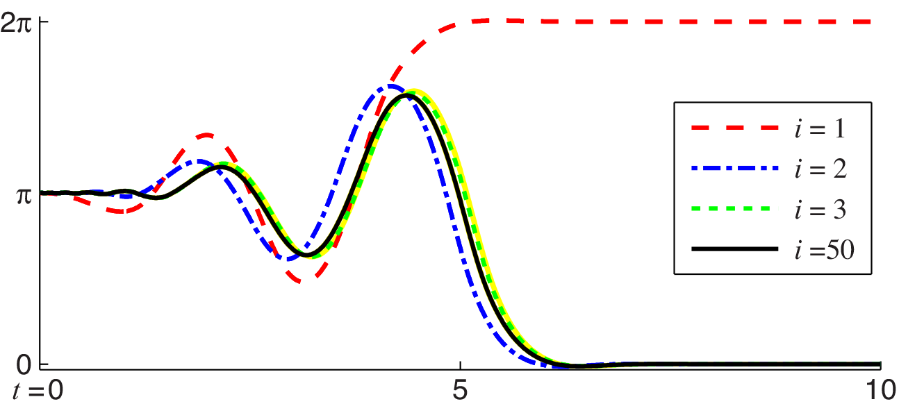
(a) Case 1: concave Hamiltonian with bounded reward — DPI

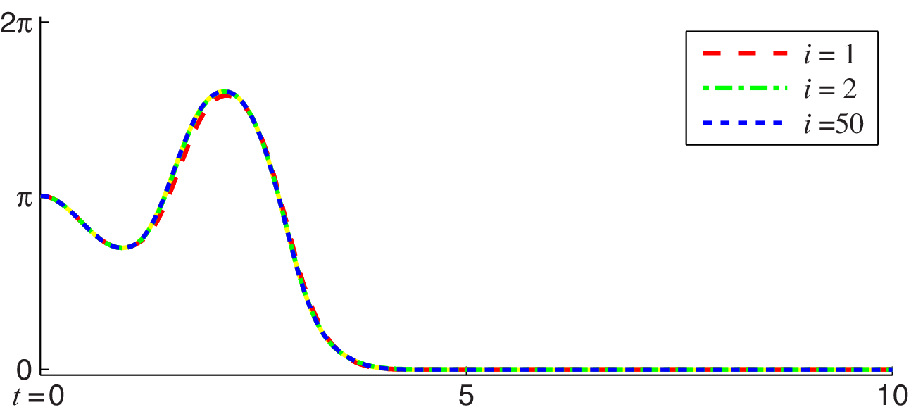
(b) Case 2: optimal control — DPI

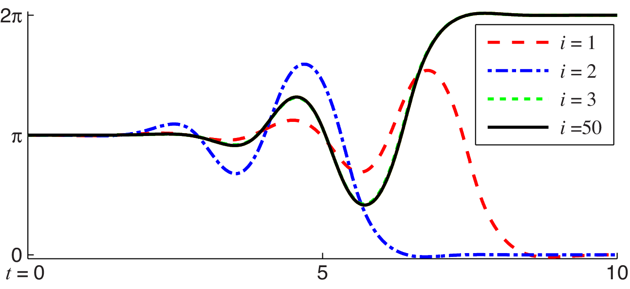
(c) Case 1: concave Hamiltonian with bounded reward —IPI

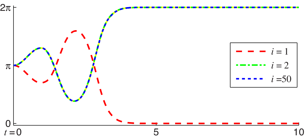
(d) Case 3: bang-bang control — IPI with $r(x,u)=\cos x_{1}$

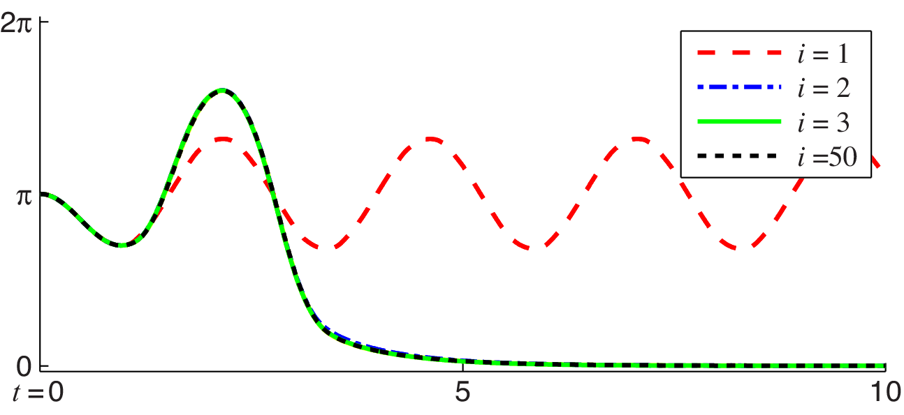
(e) Case 4: bang-bang control with binary reward – DPI

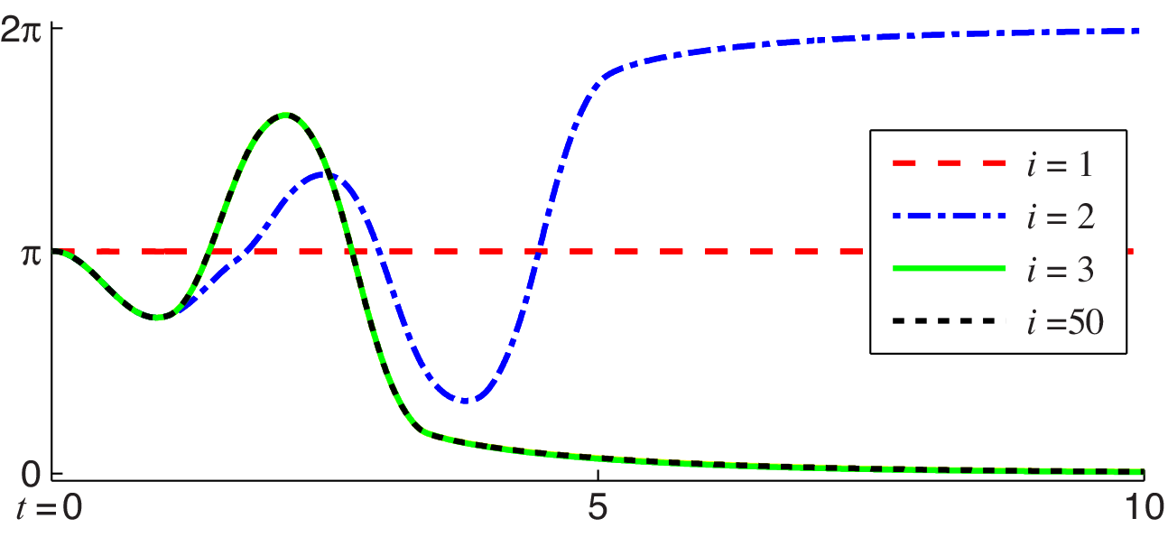
(f) Case 4: bang-bang control with binary reward – IPI

Figure 1: The trajectories of the pendulum angular-position $\vartheta_{t}$ generated by the policies obtained during and after the PIs for each case study. All of the trajectories start from $X_{0}=(\pi,0)$, and the yellow regions correspond to those $\vartheta_{t}$-trajectories at iterations $i=(3),4,5,\cdots,49$.

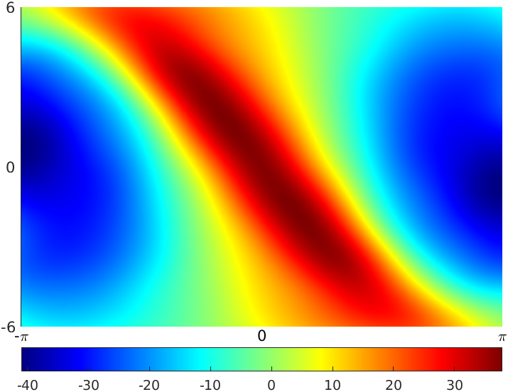
(a) ${\hat{V}}_{50}$ in Case 1 — DPI

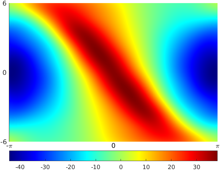
(b) ${\hat{V}}_{50}$ in Case 1 — IPI

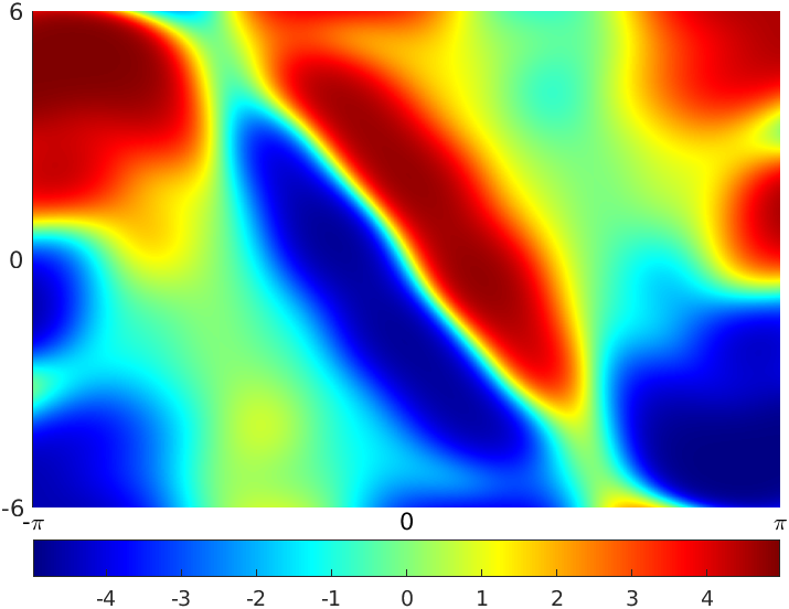
(c) ${\hat{\pi}}_{50}$ in Case 1 — DPI

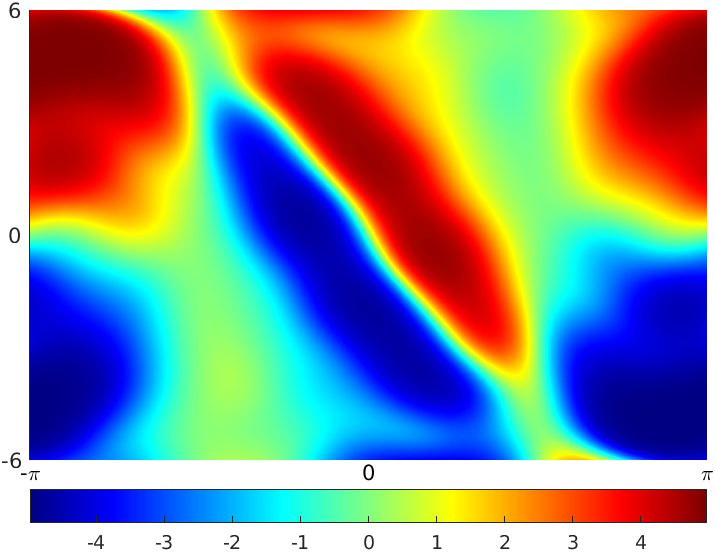
(d) ${\hat{\pi}}_{50}$ in Case 1 — IPI

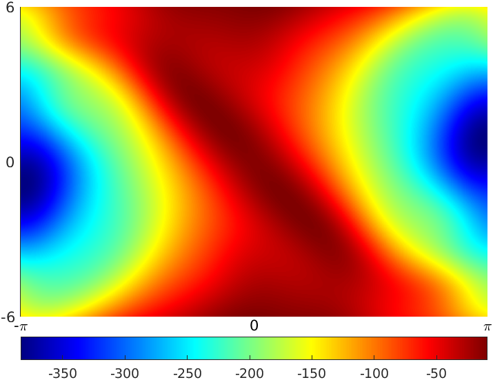
(e) ${\hat{V}}_{50}$ in Case 2 — DPI

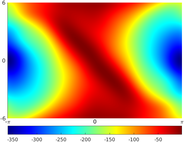
(f) ${\hat{V}}_{50}$ in Case 3 — IPI w/ (47)

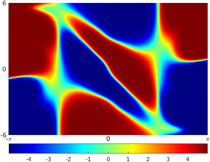
(g) ${\hat{\pi}}_{50}$ in Case 2 — DPI

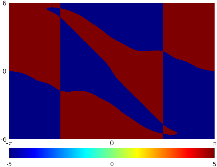
(h) ${\hat{\pi}}_{50}$ in Case 3 — IPI w/ (47)

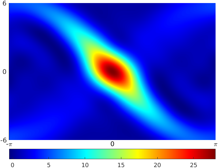
(i) ${\hat{V}}_{50}$ in Case 4 — DPI

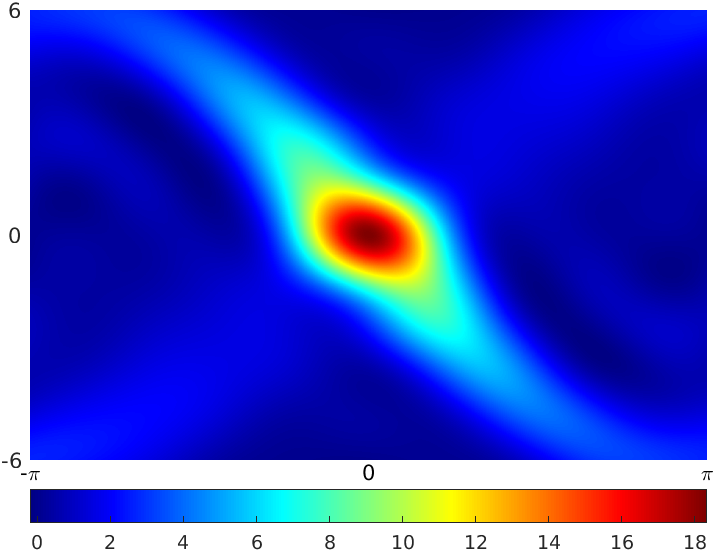
(j) ${\hat{V}}_{50}$ in Case 4 — IPI

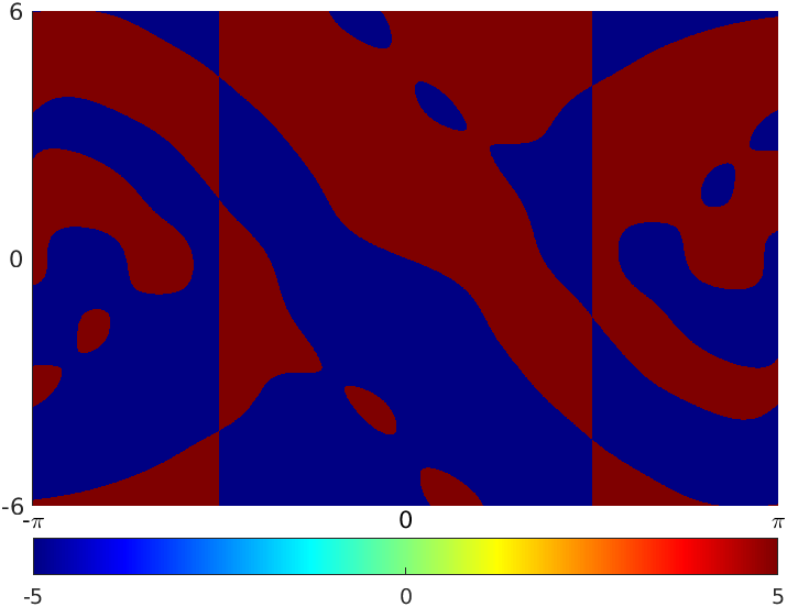
(k) ${\hat{\pi}}_{50}$ in Case 4 — DPI

Figure 2: The optimal value function ${\hat{V}}_{50}(x)=V(x;\theta_{i}^{*})|_{i=50}$ (left sides) and the optimal policy ${\hat{\pi}}_{50}(x)=\pi(x;\theta_{i}^{*})|_{i=50}$ (right sides), estimated by DPI and IPI variants over $\Omega$. The horizontal and vertical axes correspond to $x_{1}$ ($=\vartheta$) and $x_{2}$ ($={\dot{\vartheta}}$), respectively.

[6.6pt]($\ell$) ${\hat{\pi}}_{50}$ in Case 4 — IPI

6 Inverted-Pendulum Simulation Examples

section:simulation

To support the theory and further investigate the proposed PI methods, we simulate the variants of DPI and IPI shown in Algorithm 3 applied to an inverted-pendulum model:

$${\ddot{\vartheta}}_{t}=-0.01{\dot{\vartheta}}_{t}+9.8\sin\vartheta_{t}-U_{t}\cos\vartheta_{t},$$

where $\vartheta_{t}\in\mathbb{R}$ and $U_{t}\in\mathcal{U}$ are the angular position of and the external torque input to the pendulum at time $t$, respectively; the action space is given by $\mathcal{U}=[-u_{\mathsf{max}},u_{\mathsf{max}}]\subset\mathbb{R}$, with the torque limit $u_{\mathsf{max}}=5$ [N$\cdot$m]. Letting $X_{t}\doteq[\,\vartheta_{t}\;\,{\dot{\vartheta}}_{t}\,]^{\mathsf{T}}$, then the dynamics can be expressed as (1) and (29) with

$$f_{\mathsf{d}}(x)=\begin{bmatrix}x_{2}\\ 9.8\,\sin x_{1}-0.01x_{2}\end{bmatrix}\textrm{ and }F_{\mathsf{c}}(x)=\begin{bmatrix}0\\ -\cos x_{1}\end{bmatrix},$$

where $x=[\,x_{1}\,\;x_{2}\,]^{\mathsf{T}}\in\mathcal{X}$ ($=\mathbb{R}^{2}$). In the simulations, we set the discount factor $\gamma=0.1$ and the time step $\Delta t=10$ [ms]; the zero initial policy $\pi_{0}(x)\equiv 0$ is employed.

The solution $V_{i}$ of the policy evaluation at each iteration $i$ is represented by a linear function approximator $V$ as

$$V_{i}(x)\approx V(x;\theta_{i})\doteq\theta_{i}^{\mathsf{T}}\phi(x),$$ (44)

for its weights $\theta_{i}\in\mathbb{R}^{L}$ and features $\phi:\mathcal{X}\to\mathbb{R}^{L}$, with $L=121$. Each policy evaluation determines $\theta_{i}$ by the least-squares solution $\theta_{i}^{*}$ minimizing the Bellman errors over the set of initial states uniformly distributed as the ($N\times M$)-grid points over the region $\Omega=[-\pi,\pi]\times\![-6,6]\subset\mathcal{X}$. Here, $N$ and $M$ are the total numbers of the grids in the $x_{1}$- and $x_{2}$-directions, respectively; we choose $N=20$ and $M=21$, so the total $420$ number of grid points in $\Omega$ are used as initial states. When inputting to $V$, the first component $x_{1}$ of $x$ is normalized to a value within $[-\pi,\pi]$ by adding $\pm 2\pi k$ to it for some $k\in\mathbb{Z}$.

In what follows, we simulate four different settings, whose learning objective is to swing up and eventually settle down the pendulum at the upright position $\theta_{t}=2\pi k$ for some $k\in\mathbb{Z}$, under the torque limit $|U_{t}|\leq u_{\mathsf{max}}$. For each case, we basically consider the reward function $r$ given by (30) and (33) with

$$s(\mathfrak{u})=u_{\mathsf{max}}\tanh(\mathfrak{u}/u_{\mathsf{max}}).$$ (45)

As the inverted pendulum dynamics is input-affine, this setting corresponds to the concave Hamiltonian formulation in §5.1.1 (with a bounded $r$ if $\mathfrak{r}$ is bounded). The implementation details (the features $\phi$, policy evaluation, and policy improvement) are provided in §H; the MATLAB/Octave source code for the simulations is also available online.

6.1 Case 1: Concave Hamiltonian with Bounded Reward

subsection:simulation:case1

First, we consider the reward function $r$ given by (30) and (33) with $s(\cdot)$ given by (45), $\Gamma=10^{-2}$, and $\mathfrak{r}(x)=\cos x_{1}$. As mentioned above, this setting corresponds to the concave Hamiltonian formulation in §LABEL:subsection:RL_under_u-AC_setting, resulting in the following policy improvement update rule (see §H for details):

$$\!\!\!\!\!\pi_{i}(x)\approx\pi(x;\theta_{i}^{*})=-5\tanh\!\big{(}\!\cos x_{1}\!\cdot\!\nabla_{\!x_{2}}\phi(x)\!\cdot\!\theta_{i}^{*}/5\big{)}.$$ (46)

As $\mathfrak{r}$ (hence $r$) is bounded, this setting also corresponds to “discounted RL under Assumption 5.8” in §LABEL:subsection:discounted_RL_with_bounded_v. Therefore, the initial and subsequent VFs in PIs are all bounded; the properties in §§5.1.1 and LABEL:subsection:discounted_RL_with_bounded_v are all true; the Assumptions in Table 1 w.r.t. §§5.1.1 and LABEL:subsection:discounted_RL_with_bounded_v are also all relaxed.

Figs. 1(a), (c) and Figs. 2k(a)–(d) show the trajectories of $\vartheta_{t}$ under the policies obtained during PI and the estimates of the optimal solution $(v_{*},\pi_{*}$) finally obtained at the iteration $i=50$, respectively; the yellow regions in Fig. 1 correspond to the trajectories of $\vartheta_{t}$ generated by the intermediate policies obtained by the PIs at iterations $i=(3),4,5,\cdots,49$. Although both DPI and IPI variants generate rather different trajectories of $\vartheta_{t}$ in Figs. 1(a), (c), due to the difference in the estimates of the VF and policy (e.g., see Figs. 2k(a)–(d)), both methods have achieved the learning objective merely after the first iteration. Here, the difference in the $\vartheta_{t}$-trajectories mainly comes from the different initial behaviors near $\vartheta=\pi$ — see the differences in the policies in Figs. 2k(c), (d) (and also the VF estimates in Figs. 2k(a), (b)) near the borderlines $\vartheta=\pm\pi$. Also note that both DPI and IPI methods have achieved our learning objective without using an initial stabilizing policy that is usually required in the optimal control setting under the total discounting $\gamma=1$ (e.g., Abu-Khalaf and Lewis, 2005; Vrabie and Lewis, 2009; Lee et al., 2015).

6.2 Case 2: Optimal Control

subsection:simulation:case2 A better performance can be obtained if the state reward function $\mathfrak{r}$ in Case 1 is replaced by

$$\mathfrak{r}(x)=-x_{1}^{2}-\epsilon\!\cdot\!x_{2}^{2}\;\;\,\textrm{ with }\epsilon=10^{-2}.$$

This setting corresponds to the nonlinear optimal control introduced and discussed in §LABEL:subsection:nonlinear_optimal_control. In this case, whenever input to $\mathfrak{r}$, the first component $x_{1}$ is normalized to a value within $[-\pi,\pi]$. Here, $\mathfrak{r}$ is still not bounded due to the existence of the term $-\epsilon\cdot x_{2}^{2}$, but Algorithm 3 (without assuming the boundedness of $\smash{v}_{\pi_{0}}$) can be successfully applied as shown in Figs. 1(b), 2k(e), and 2k(g). Fig. 1(b) illustrates the trajectories of $\vartheta_{t}$ under the policies obtained by the DPI variant. Compared with Case 1, this setting gives a better initial and asymptotic performance — every trajectory of $\vartheta_{t}$ in Fig. 1(b) is almost the same as the final one (faster convergence of the PI) and converges to the goal state $x=(0,0)$ more rapidly than any trajectories of $\vartheta_{t}$ in Case 1. In particular, the initial behavior near $\vartheta=\pm\pi$ has been improved, so that the policies in this case swing up the pendulum much faster than Case 1. One possible explanation about this is that the higher magnitude of the gradient of $\mathfrak{r}$ near $x_{1}=\pm\pi$ expedites the initial swing-up process (note, in Case 1, $\nabla\mathfrak{r}(\pm\pi,x_{2})=0$ for any $x_{2}$). See also the difference of the final VF and policy in Figs. 2k(e), (g) (Case 2) from those in Figs. 2k(a)–(d) (Case 1). The results for IPI are almost similar to DPI in this case, so their figures are omitted.

6.3 Case 3: Bang-bang Control

subsection:simulation:case3 If $\Gamma\to 0$, the reward function $r$ and the policy update rule (46) in Case 1 (§LABEL:subsection:simulation:case1) are simplified to $r(x,u)=\cos x_{1}$ and

$$\pi_{i}(x)\approx\pi(x;\theta_{i}^{*})=-5\cdot\mathrm{sign}\big{(}\cos x_{1}\!\cdot\!\nabla_{\!x_{2}}\phi(x)\cdot\theta_{i}^{*}\big{)}$$

(see §H for details), a bang-bang type discrete control. The PI methods can be also applied to optimize this bang-bang type controller. Note that this case is beyond our scope of the theory developed in §§LABEL:section:preliminaries–LABEL:section:case_studies since the policy is discrete, not continuous. For this bang-bang control framework, Fig. 1(d) shows the $\vartheta_{t}$-trajectories under the discrete policies obtained by the IPI variant in Algorithm 3. Though the fast switching behavior of the control $U_{t}$ is inevitable near $x=(0,0)$, due to $\mathrm{sign}(\cdot)$, the initial and asymptotic control performance, compared with Case 1, has been increased in the limit $\Gamma\to 0$ up to the performance of optimal control (Case 2).

By limiting $\Gamma\to 0$, the control policy in Case 2 can be also made a bang-bang type control, but in this case, with

$$r(x,u)=-x_{1}^{2}-\epsilon\!\cdot\!x_{2}^{2}\;\;\textrm{ with }\epsilon=10^{-2}.$$ (47)

We have observed that the performance of the PI methods in this case is almost same as that shown in Fig. 1(d) for the previous case “$r(x,u)=\cos x_{1}$”, derived from Case 1. Figs. 2k(f) and (h) show the envelopes of the VF and the bang-bang policy under (47), both of which are consistent with the envelopes for $\Gamma=10^{-2}$ shown in Figs. 2k(e) and (g).

6.4 Case 4: Bang-bang Control with Binary Reward

subsection:sim:bang-bang with binary

In RL problems, the reward is often binary and sparely given only at or near the goal state. To investigate this case, we also consider the bang-bang policy given in the previous subsection, but with the binary reward function:

$$r(x,u)=\begin{cases}1,\textrm{ if }|x_{1}|\leq 6/\pi\textrm{ and }|x_{2}|\leq 1/2\\[5.0pt] 0,\textrm{ otherwise,}\end{cases}$$

This gives the reward signal $R_{t}=1$ near the goal state $x=(0,0)$ only. Figs. 1(e) and (f) illustrate the $\theta_{t}$-trajectories under the policies generated by the DPI and IPI variants (i.e., Algorithm 3), respectively. Though the initial performance is neither stable ($i=1$) nor consistent to each other ($i=1,2$), both PI methods eventually converge to the same seemingly near-optimal point ($i=3,4,\cdots,50$). Note that the performance after learning ($i=50$) for both cases is the same as that of Cases 2 and 3 until around $t=3[s]$ as can be seen from Figs. 1(b) and (d)–(f). Figs. 2k(i)–($\ell$) also show the estimates of the optimal VF and policy at $i=50$. Although the details are a bit different, we can see that both methods finally result in similar consistent estimates of the VF and policy. In this binary reward case, the shapes of the VF shown in Figs. 2k(i) and (j) are distinguished from the others illustrated in Figs. 2k(a),(b),(e), and (f) due to the reward information condensed near the goal state $x=(0,0)$ only. Even in this situation, our PI methods were able to achieve the goal at the end, as shown in Figs. 1(e) and (f). For the DPI variant, we have simulated this case with $M=20$, instead of $M=21$.

6.5 Discussions

subsection:sim:discussions

We have simulated the variants of DPI and IPI (Algorithm 3) under the four scenarios above. Some of them have achieved the learning objective immediately at the first iteration, and in all of the simulations, the proposed methods were able to achieve the goal, eventually. On the other hand, the implementations of the PIs have the following issues.

1. The least-squares solution $\theta_{i}^{*}$ of each policy evaluation minimizes the Bellman error over a finite number of initial states in $\Omega$ (as detailed in §H), meaning that it is not the optimal choice to minimize the Bellman error over the entire region $\Omega$. As mentioned in §LABEL:section:PIs, the ideal policy evaluation cannot be implemented precisely—even when $\Omega$ is compact, it is a continuous space and thus contains an (uncountably) infinite number of points that we cannot fully cover in practice.
   

2. As the dimension of the data matrix in the least squares is $L\times(NM)=121\times 420$ (see §H), calculating the least-squares solution $\theta_{i}^{*}$ is computationally expensive, and the numerical error (and thus the convergence) is sensitive to the choice of the parameters such as (the number of) the features $\phi$, the time step $\Delta t$, discounting factor $\gamma$, and of course, $N$ and $M$. In our experiments, we have observed that Case 2 (optimal control) was least sensitive to those parameters.
   

3. The VF parameterization. Since the pendulum is symmetric at $x_{1}=0$, the VFs and policies obtained in Fig 2k are all symmetric, and thus it might be sufficient to approximate the VF over $[0,\pi]\times[-6,6]\subset\Omega$, with a less number of weights, and use the symmetry of the problem. Due to the over-parameterization, we have observed that the weight vector $\theta_{i}^{*}$ in certain situations never converges but oscillates between two values, even after the VF $V_{i}$ has almost converged over $\Omega$.

All of these algorithmic and practical issues are beyond the scope of this paper and remain as a future work.

7 Conclusions

section:conclusion  
In this paper, we proposed fundamental PI schemes called DPI (model-based) and IPI (partially model-free) to solve the general RL problem formulated in CTS. We proved their fundamental mathematical properties: admissibility, uniqueness of the solution to the BE, monotone improvement, convergence, and the optimality of the solution to the HJBE. Strong connections to the RL methods in CTS—TD learning and VGB greedy policy update—were made by providing the proposed ones as their ideal PIs. Case studies simplified and improved the proposed PI methods and the theory for them, with strong connections to RL and optimal control in CTS. Numerical simulations were conducted with model-based and partially model-free implementations to support the theory and further investigate the proposed PI methods beyond, under an initial policy that is admissible but not stable. Unlike the existing PI methods in the stability-based frameworks, an initial stabilizing policy is not necessarily required to run the proposed ones. We believe that this work provides the theoretical background, intuition, and improvement to both (i) PI methods in optimal control and (ii) RL methods, to be developed in the future and developed so far in CTS domain.

Abstract

This supplementary document provides additional studies and all the details of the contents presented by Lee and Sutton (2020), as listed below. Roughly speaking, we present related works, details of the theory, algorithms, and implementations, additional case studies, and all the proofs, with the same abbreviations, terminologies, and notations. All the numbers of equations, sections, theorems, lemmas, etc. that do not contain any alphabet will refer to those in the main paper (Lee and Sutton, 2020), whereas any numbers starting with an alphabet correspond to those in the Appendices herein.

Appendix A Notations and Terminologies

We provide a complete list of notations and terminologies used in the main paper and the appendices. In any statement, iff and s.t. stand for if and only if and such that, respectively. “$\doteq$” denotes the equality relationship that is true by definition.

A.1 Abbreviations

ADP	approximate dynamic programming
BE	Bellman equation
CTS	continuous time and space
DPI	differential policy iteration
IPI	integral policy iteration
HJB	Hamilton-Jacobi-Bellman
HJBE	Hamilton-Jacobi-Bellman equation
LQR	linear quadratic regulation
MDP	Markov decision process
ODE	ordinary differential equation
PI	policy iteration
RBF	radial basis function
RL	reinforcement learning
TD	temporal difference
VF	value function
VGB	value-gradient-based

A.2 Sets, Vectors, and Matrices

$\mathbb{N}$	set of all natural numbers
$\mathbb{R}$	set of all real numbers
$\mathbb{C}$	set of all complex numbers
$\mathbb{Z}$	set of all integers
$\mathbb{R}^{n\times m}$	set of all $n$-by-$m$ real matrices
$\mathbb{R}^{n}$	$n$-dimensional Euclidean space $\doteq\mathbb{R}^{n\times 1}$

For a matrix $A\in\mathbb{R}^{n\times m}$ and a vector $x\in\mathbb{R}^{m}$,

$A^{\mathsf{T}}$	transpose of $A$
$\operatorname{\rm rank}\left(A\right)$	rank of $A$
$\|x\|$	Euclidean norm of $x$, i.e., $\|x\|\doteq(x^{\mathsf{T}}x)^{1/2}$
$\|x\|_{\Omega}$	distance of $x$ from a subset $\Omega\subset\mathbb{R}^{m}$, i.e., $\|x\|_{\Omega}\doteq\inf\{\|x-y\|:y\in\Omega\}$
${\left|\kern-1.07639pt\left|\kern-1.07639pt\left|A\right|\kern-1.07639pt\right|\kern-1.07639pt\right|}$	induced norm of $A$, i.e., ${\left|\kern-1.07639pt\left|\kern-1.07639pt\left|A\right|\kern-1.07639pt\right|\kern-1.07639pt\right|}\doteq{\displaystyle\sup_{\smash{\|}x\|=1}}\|Ax\|$
$I$	identity matrix with a compatible dimension

A.3 Euclidean Topology

Let $\Omega\subseteq\mathbb{R}^{n}$.

${\kern 0.0pt\Omega}^{\mathrm{o}}$ denotes the interior of $\Omega$.

$\partial{\kern 0.0pt\Omega}$ denotes the boundary of $\Omega$.

$\Omega$ is said to be compact iff it is closed and bounded.

If $\Omega$ is open, then $\Omega\cup\partial{\kern 0.0pt\Omega}$ (resp. $\Omega$) is called an $n$-dimensional manifold with (resp. without) boundary. By this definition, a manifold contains no isolated point.

A.4 Functions, Sequences, and Convergence

Let $\Omega\subseteq\mathbb{R}^{n}$ and $f:\Omega\to\mathbb{R}^{m}$ be a function.

$f\in\mathrm{C}^{k}$ (i.e., $f$ is $\mathrm{C}^{k}$) iff the $k$th order partial derivatives of $f$ all exist and are continuous, over the interior ${\kern 0.0pt\Omega}^{\mathrm{o}}$.

$\nabla f:{\kern 0.0pt\Omega}^{\mathrm{o}}\to\mathbb{R}^{m\times n}$ denotes the gradient of $f$.

$f$ is locally Lipschitz iff for each $x\in\Omega$, there exists $L>0$ and a neighborhood $\mathcal{N}_{x}$ of $x$ s.t. for all $y,z\in\mathcal{N}_{x}$,

$$\|f(y)-f(z)\|\leq L\|y-z\|.$$ (48)

$f$ is globally Lipschitz iff $\exists L>0$ s.t. (48) holds $\forall y,z\in\Omega$.

$f\in\mathrm{C}^{1}_{\mathsf{Lip}}$ (i.e., $f$ is $\mathrm{C}^{1}_{\mathsf{Lip}}$) iff $f$ is locally Lipschitz and $\mathrm{C}^{1}$.

$f$ is odd iff $f(-x)=f(x)$ for all $x\in\Omega$.

$f$ with $m=n$ is strictly monotone iff for each $x$, $x^{\prime}\in\Omega$,

$$(f(x)-f(x^{\prime}))^{\mathsf{T}}(x-x^{\prime})>0\text{ whenever }x\neq x^{\prime}.$$

$f(E)\doteq\{f(x):x\in E\}$, the image of $E\subseteq\Omega$ under $f$.

A sequence $\langle a_{i}\rangle_{i=1}^{\infty}$ is abbreviated as $\langle a_{i}\rangle$ or $a_{i}$ for notational simplicity. A sequence of functions $\langle f_{i}\rangle$ converges (to $f$)

pointwise iff $f_{i}(x)\to f(x)$ for each $x\in\Omega$;

uniformly on $E\subseteq\Omega$ iff $\sup_{x\in E}\|f_{i}(x)-f(x)\|\to 0$;

locally uniformly iff for each $x\in\Omega$, there is a neighborhood of $x$ on which $f_{i}\to f$ uniformly.

For any two functions $f_{1},f_{2}:\mathbb{R}^{n}\to[-\infty,\infty)$, we write

$$f_{1}\leqslant f_{2}\;\,\Longleftrightarrow\;\,f_{1}(x)\leq f_{2}(x)\quad x\in\mathbb{R}^{n}.$$

A function $f:\Omega\to\mathbb{R}$ is said to be

positive semidefinite iff $f(0)=0$ and $f\geqslant 0$;

negative semidefinite iff $-v$ is positive semidefinite;

positive definite iff $f(0)=0$ and $f(x)>0$ for all $x\neq 0$;

negative definite iff $-f$ is positive definite;

radially unbounded iff $\inf_{\|x\|\geq r}|f(x)|\to\infty$ as $r\to\infty$;

radially nonvanishing iff $\inf_{\|x\|\geq r}|f(x)|\not\to 0$ as $r\to\infty$;

convex iff for each $x,x^{\prime}\in\Omega$ and $\beta\in(0,1)$,

• $x_{\beta}\doteq\beta x+(1-\beta)x^{\prime}\in\Omega$ (i.e., $\Omega$ is convex),

• $f(x_{\beta})\leq\beta\cdot f(x)+(1-\beta)\cdot f(x^{\prime})$;

concave iff $-f$ is convex;

strictly convex iff $f$ is convex and for any $\beta\in(0,1)$,

$$f(x_{\beta})<\beta\cdot f(x)+(1-\beta)\cdot f(x^{\prime})\textrm{ whenever }x\neq x^{\prime};$$

strictly concave iff $-f$ is strictly convex.

$f:[0,\infty)\to[0,\infty)$ is said to be $\mathcal{K}_{\infty}$ iff $f(0)=0$ and $f$ is strictly increasing, radially unbounded, and continuous;

A square matrix $P\in\mathbb{R}^{n\times n}$ is

positive (semi)definite iff so is $z\mapsto z^{\mathsf{T}}Pz$ and $P^{\mathsf{T}}=P$;

negative (semi)definite iff so is $z\mapsto z^{\mathsf{T}}Pz$ and $P^{\mathsf{T}}=P$.

For $P,P^{\prime}\in\mathbb{R}^{n\times n}$, we denote $P<P^{\prime}$ (resp. $P\leq P^{\prime}$) iff $P^{\prime}-P$ is positive definite (resp. positive semidefinite).

A.5 Reinforcement Learning

$l$	dimension $\in\mathbb{N}$ of the state space $\mathcal{X}$
$m$	dimension $\in\mathbb{N}$ of action spaces (e.g., $\mathcal{U}$ and $\mathcal{A}$)

An action space is an $m$-dimensional manifold in $\mathbb{R}^{m}$ with or without boundary hence has no isolated point by definition.

$\mathcal{X}$, $\mathcal{X}^{\mathsf{T}}$	state space $\mathcal{X}\doteq\mathbb{R}^{l}$ and $\mathcal{X}^{\mathsf{T}}\doteq\mathbb{R}^{1\times l}$
$\mathcal{U}$	action space $\subseteq\mathbb{R}^{m}$
$\mathcal{A}$	a transformed action space $\subseteq\mathbb{R}^{m}$ (§§LABEL:subsection:RL_under_u-AC_setting and G.1)
$\mathbb{T}$	time space $\mathbb{T}\doteq[0,\infty)$

$f$, $f^{x}$	dynamics $f:\mathcal{X}\times\mathcal{U}\to\mathcal{X}$ and $f^{x}(u)\doteq f(x,u)$
$f_{\mathsf{d}}$	drift dynamics $f_{\mathsf{d}}:\mathcal{X}\to\mathcal{X}$
$f_{\mathsf{c}}$	input-coupling dynamics $f_{\mathsf{c}}:\mathcal{X}\times\mathcal{U}\to\mathcal{X}$
$F_{\mathsf{c}}$	input-coupling matrix $F_{\mathsf{c}}:\mathcal{X}\to\mathbb{R}^{n\times m}$ (§LABEL:subsection:RL_under_u-AC_setting)
$r$, $r^{x}$	reward function $r:\mathcal{X}\times\mathcal{U}\to\mathbb{R}$; $r^{x}(u)\doteq r(x,u)$
$r_{\mathsf{max}}$	the reward maximum “$\max_{(x,u)}r(x,u)$”
$\gamma$	discount factor $\in(0,1]$
$\alpha$	attenuation rate $\alpha\doteq-\ln\gamma\geq 0$
$h$	Hamiltonian function $h:\mathcal{X}\times\mathcal{U}\times\mathcal{X}^{\mathsf{T}}\to\mathbb{R}$
$u_{*}$	maximal function $u_{*}(x,p)\in\operatorname*{arg\,max}_{u}h(x,u,p)$

$t$	time variable $\in\mathbb{T}$
$\eta$	time horizon $\in(0,\infty]$
$X_{t}$	state vector $\in\mathcal{X}$ at time $t$
${\dot{X}}_{t}$	the time derivative $\in\mathcal{X}$ of $X_{t}$ at time $t$
$U_{t}$	action (also called control) vector $\in\mathcal{U}$ at time $t$
$A_{t}$	a transformed action vector $\in\mathcal{A}$ at time $t$
$R_{t}$	reward at time $t$, i.e., $r(X_{t},U_{t})\in\mathbb{R}$
$\mathfrak{R}_{\eta}$	discounted cumulative reward up to horizon $\eta$
${\dot{v}}$	time derivative $dv(X_{t})/dt=\nabla v(X_{t})f(X_{t},U_{t})$

A policy is a continuous function from $\mathcal{X}$ to $\mathcal{U}$; for a policy $\pi$,

$\mathbb{G}_{\pi}^{x}[Y]$	value $Y$ when $X_{0}=x$ and $U_{t}=\pi(X_{t})$ $\forall t\in\mathbb{T}$
$v_{\pi}$	value function (VF) with respect to $\pi$
$\macc@depth\char 1\relax\frozen@everymath{\macc@group}\macc@set@skewchar\macc@nested@a 111{v}$	a uniform upper-bound of VFs ($\bar{v}=0$ for $\gamma=1$        and $\bar{v}=r_{\mathsf{max}}/\alpha$ otherwise — see Lemma 2.1)
$f_{\pi}$	closed-loop dynamics $f_{\pi}(x)\doteq f(x,\pi(x))$
$r_{\pi}$	closed-loop reward function $r_{\pi}(x)\doteq r(x,\pi(x))$
$\pi^{\prime}$	an improved/maximal policy $\pi^{\prime}\!\succcurlyeq\pi$, i.e., $v_{\pi^{\prime}}\!\geqslant v_{\pi}$

When $f_{\pi}$ is locally Lipschitz, $t_{\mathsf{max}}(x;\pi)$ denotes the minimal time s.t. $\forall t\geq t_{\mathsf{max}}(x;\pi)$, no state $\mathbb{G}_{\pi}^{x}[X_{t}]$ exists (§LABEL:subsection:RL_with_local_Lipschitzness).

$\Pi_{\mathsf{a}}$	set of all admissible policies
$\Pi_{\mathsf{Lip}}$	set of all locally Lipschitz policies
$\mathcal{V}_{\mathsf{a}}$	set of all admissible VFs
$d$, $d_{\Omega}$	a metric and the uniform pseudometric, on $\mathcal{V}_{\mathsf{a}}$
$\mathcal{T}$	the PI operator
$v_{*}$	a solution to the HJBE or the optimal VF
$v^{*}$	a (unique) fixed point of $\mathcal{T}$
$\pi_{*}$	an HJB or optimal policy (or a function $\pi_{*}$ that satisfies (17) and is potentially discontinuous).

A.6 Policy Iteration

$i$	iteration index $\in\mathbb{N}$
$v_{i}$, $V_{i}$	solution to the BE at iteration $i$; $V_{i}\doteq v_{i}/\Delta t$
${\hat{v}}_{*}$	limit function ${\hat{v}}_{*}(x)\doteq\sup_{i}v_{i}(x)={\displaystyle\lim_{i\to\infty}}v_{i}(x)$
$\pi_{0}$, $\pi_{i}$	an initial policy and the policy at iteration $i$
$\Delta t$	small time step $(0<\Delta t\ll 1)$
$\gamma_{\mathsf{d}}$	discount factor $\doteq\gamma^{\Delta t}$ in discrete time
${\hat{\gamma}}_{\mathsf{d}}$	an approximation of $\gamma_{\mathsf{d}}\approx{\hat{\gamma}}_{\mathsf{d}}\doteq 1-\alpha_{\mathsf{d}}$
$\alpha_{\mathsf{d}}$	attenuation rate $\doteq\alpha\Delta t=-\ln\gamma_{\mathsf{d}}$ in discrete time

A.7 Optimal Control and LQRs

$c$	cost function $c\doteq-r$
$c_{\pi}$	closed-loop cost function $c_{\pi}(x)\doteq c(x,\pi(x))$
$C_{t}$	cost at time $t$, i.e., $c(X_{t},U_{t})\in\mathbb{R}$
$J_{\pi}$	cost value function $J_{\pi}\doteq-v_{\pi}$
$J_{i}$, $J_{*}$	$J_{i}\doteq-v_{i}$ and $J_{*}\doteq-v_{*}$
$\Pi_{0}$	set of all policies $\pi\in\Pi_{\mathsf{Lip}}$ s.t. $\pi(0)=0$

Let $A\in\mathbb{R}^{l\times l}$, $B\in\mathbb{R}^{m\times l}$, and $C\in\mathbb{R}^{p\times l}$. Then,

$A$ is Hurwitz iff every eigenvalue has a negative real part;

$(A,B)$ stabilizable iff $\exists K\in\mathbb{R}^{m\times l}$ s.t. $A-BK$ is Hurwitz;

$(C,A)$ observable iff for any $\eta>0$, the initial state $X_{0}$ can be determined from the history $\{(CX_{t},U_{t})\}_{t\in[0,\eta]}$, where $\{X_{t}\}_{t\in[0,\eta]}$ satisfies ${\dot{X}}_{t}=AX_{t}+BU_{t}$.

Appendix B Highlights and Related Works

First, we briefly review the related works from RL and optimal control fields. We also highlight the main aspects of (i) the proposed PI methods and the underlying theory, both developed by Lee and Sutton (2020), and (ii) the appendices herein.

DPI & IPI. Two main PI methods in our work are DPI, whose policy evaluation is associated with the differential BE, and IPI associated with the integral BE. The former was inspired by the model-based PI methods in optimal control (e.g., Rekasius, 1964; Leake and Liu, 1967; Saridis and Lee, 1979; Beard et al., 1997; Abu-Khalaf and Lewis, 2005; Bian et al., 2014) and has a direct connection to TD(0) in CTS (Doya, 2000; Frémaux et al., 2013) — see §LABEL:subsection:DPI. As regards to the latter, the integral BE was first introduced by Baird III (1993) in the field of RL and then spotlighted in the optimal control community, resulting in a series of IPI methods applied to a class of input-affine dynamics for optimal regulations (Vrabie and Lewis, 2009; Lee et al., 2015), robust control (Wang, Li, Liu, and Mu, 2016), and (discounted) LQ tracking control (Modares and Lewis, 2014; Zhu, Modares, Peen, Lewis, and Yue, 2015; Modares et al., 2016), with a number of extensions to off-policy IPI methods (e.g., Bian et al., 2014; Lee et al., 2015; Wang et al., 2016; Modares et al., 2016). In our work (Lee and Sutton, 2020),

1. the proposed IPI was motivated by the first IPI given by Vrabie and Lewis (2009) for nonlinear optimal regulations;

2. the ideas of DPI and IPI have generalized for a broad class of dynamics and reward functions in CTS shown in §LABEL:section:preliminaries, which includes the existing RL tasks (Doya, 2000; Mehta and Meyn, 2009; Frémaux et al., 2013) and the case tasks of RL and optimal control presented in §§LABEL:section:case_studies and G.

Case Studies.

1. (§LABEL:subsection:RL_under_u-AC_setting. Concave Hamiltonian Formulation). A highlight is in §LABEL:subsection:RL_under_u-AC_setting, which draws the connection to the VGB greedy policy update (Doya, 2000), a general idea of simplifying policy improvement in input-constrained RL problems. There exist similar ideas in the optimal control field for input-constrained (Lyashevskiy, 1996; Abu-Khalaf and Lewis, 2005) and unconstrained optimal regulations (Rekasius, 1964; Saridis and Lee, 1979; Beard et al., 1997; Abu-Khalaf and Lewis, 2005; Vrabie and Lewis, 2009; Lee et al., 2015) under input-affine dynamics, and even for the non-affine dynamics (Bian et al., 2014; Kiumarsi et al., 2016).

2. (§LABEL:subsection:nonlinear_optimal_control. Nonlinear Optimal Control). The existing PI methods for the optimal regulations, presented in the literature above and by Leake and Liu (1967), are strongly linked to §LABEL:subsection:nonlinear_optimal_control, where we case-studied asymptotic stability and fundamental properties of DPI and IPI applied to a general optimal regulation problem with non-affine dynamics and $\gamma\in(0,1]$. The asymptotic stability conditions given in Theorem 5.13 in §LABEL:subsection:nonlinear_optimal_control are similar to and inspired by Gaitsgory et al. (2015, Assumptions 2.3 and 3.8).

3. (§LABEL:subsection:discounted_RL_with_bounded_v Discounted RL with Bounded VF). Another highlight is the discounted RL problem with bounded reward function (§LABEL:subsection:discounted_RL_with_bounded_v). In this case, the VF is guaranteed to be bounded for any policy, by which the underlying PI theory becomes dramatically simplified and clear (see Corollary 5.9). This framework is akin to the RL tasks in a finite MDP, where the reward defined for each state transition is bounded (Sutton and Barto, 2018).

See also §LABEL:section:simulation for simulation examples of those case studies in §LABEL:subsection:RL_under_u-AC_setting, LABEL:subsection:discounted_RL_with_bounded_v, and LABEL:subsection:nonlinear_optimal_control, for RL and optimal control.

Admissibility & Asymptotic Stability. Theoretically, since we consider a stability-free RL framework (under the minimal assumptions in §LABEL:section:preliminaries), we excluded asymptotic stability from the definition of an admissible policy. Here, the notion of admissibility in optimal control has been defined with asymptotic stability (e.g., Beard et al., 1997; Abu-Khalaf and Lewis, 2005; Vrabie and Lewis, 2009; Modares and Lewis, 2014; Bian et al., 2014; Lee et al., 2015 to name a few), and this work is the first to define admissibility in CTS without asymptotic stability. Conversely, in a general optimal control problem, we also showed that when $\gamma=1$, admissibility, according to our definition, implies asymptotic stability (if the associated VF is $\mathrm{C}^{1}$) — see Theorem 5.13 and Remarks 5.14 and 5.20 in §LABEL:subsection:nonlinear_optimal_control. This means that asymptotic stability can be removed from the definition of admissibility even in optimal control. The admissibility in discounted optimal control was also investigated in §LABEL:subsection:nonlinear_optimal_control under the condition weaker than a Lyapunov’s global asymptotic stability criterion (e.g., see Theorem 5.17).

(Mode of) Convergence. We characterized the convergence properties of the PI methods towards the optimal solution in the following three ways. Those three modes provide different convergence conditions and compensate for one another.

1. In the first characterization, we employed Bessaga (1959)’s converge fixed point principle to show that the VFs generated by the PI methods converge to the optimal one in a metric (Theorem 4.5). This first-type convergence, called convergence in a metric, is weaker than locally uniform convergence below but does not impose any other assumptions than the existence and uniqueness of a fixed point that turns out to be the optimal VF by Corollary E.2.

2. The second way was to extend the approach of Leake and Liu (1967)’s, suggesting continuity of the PI operator (see Theorem 4.6) as one of the additional conditions for locally uniform convergence.

3. Lastly, we also generalized the convergence proof from the optimal control literature (Saridis and Lee, 1979; Beard et al., 1997; Murray et al., 2002; Abu-Khalaf and Lewis, 2005; Bian et al., 2014) to our RL framework, resulting in the strongest convergence among the three, under a certain condition other than the two above (see Theorem 4.9). In this direction, we highlight that for the proof of this third type convergence, the gradients of the VFs obtained by the PIs need to be assumed to converge locally uniformly, even for the existing results in optimal control, as the convergence of the generated VFs does not imply any convergence of their derivatives (see Remark 5.2).

LQR. In §G.3, we discuss DPI and IPI applied to a class of the LQR tasks (Lancaster and Rodman, 1995, Chapter 16) where bilinear cost terms of states and controls exist. Here, DPI falls into a particular case of the existing general matrix-form PIs (Arnold III, 1984; Mehrmann, 1991), but this study slightly generalizes many existing PI methods for the LQRs (e.g., Kleinman, 1968; Vrabie et al., 2009; Lee, Park, and Choi, 2014) by taking such bilinear cost terms into considerations, with the relaxation of the positive definite matrix assumption imposed on the general matrix-form PI (Mehrmann, 1991, Theorem 11.3).

Appendix C More on the Bellman Equations with the Boundary Condition

Here, the theory on (the uniqueness of) the BEs established in §LABEL:subsection:BE_with_boundary_condition is elaborated with supplementary theorems and discussions. Let $v:\mathcal{X}\to\mathbb{R}$ be a function s.t. for a policy $\pi$, either of the followings holds:

$$\text{(1) $v$ satisfies the integral BE: }v(x)=\mathbb{G}_{\pi}^{x}\big{[}\mathfrak{R}_{\eta}+\gamma^{\eta}\!\cdot\!v(X_{\eta})\big{]}\qquad\forall x\in\mathcal{X},$$ (10)

$$\text{(2) $v$ is $\mathrm{C}^{1}$ and satisfies the differential BE: }\alpha\cdot v(x)=h(x,\pi(x),\nabla v(x))\qquad\forall x\in\mathcal{X}.$$ (11)

In §LABEL:subsection:BE_with_boundary_condition, we showed that the boundary condition (12):

$$\lim_{k\to\infty}\mathbb{G}_{\pi}^{x}\big{[}\,\gamma^{k\cdot\eta}\cdot v(X_{k\cdot\eta})\,\big{]}=0\qquad\forall x\in\mathcal{X}$$ (12)

is necessary and sufficient for the policy $\pi$ being admissible and a solution $v$ to the BE (10) or (11) being equal to the VF $v_{\pi}$. In other words, the boundary condition (12) ensures admissibility of $\pi$ and uniqueness of the solution $v$ to the BE. However, except for a few cases, (12) is hard or even impossible to check as it is a condition at infinity in time. The theorem below shows admissibility and weaker properties of the BEs but without the boundary condition (12).

Theorem C.1.

Let $\eta>0$ be fixed and suppose $v$ satisfies either the integral BE (10) or, with $v\in\mathrm{C}^{1}$, the differential BE (11). If $v$ is upper bounded (by zero if $\gamma=1$), then (i) $\pi$ is admissible and $v\leqslant v_{\pi}$; (ii) the limit in (12) exists and satisfies

$$v(x)-v_{\pi}(x)=\lim_{k\to\infty}\mathbb{G}_{\pi}^{x}\big{[}\gamma^{k\cdot\eta}\cdot v(X_{k\cdot\eta})\big{]}\leq 0\qquad\forall x\in\mathcal{X}.$$

Proof.

Suppose $v$ satisfies the integral BE (10) without loss of generality (or, convert the differential BE (11) into (10) via Lemma 2.3 and fix $\eta>0$). Then, the repetitive applications of the BE (10) to itself $k$-times result in

$$v(x)=\mathbb{G}_{\pi}^{x}\big{[}\mathfrak{R}_{\eta}+\gamma^{\eta}\!\cdot\!v(X_{\eta})\big{]}=\mathbb{G}_{\pi}^{x}\big{[}\mathfrak{R}_{2\eta}+\gamma^{2\eta}\!\cdot\!v(X_{2\eta})\big{]}=\;\,\cdots\;\,=\mathbb{G}_{\pi}^{x}\big{[}\mathfrak{R}_{k\cdot\eta}+\gamma^{k\cdot\eta}\!\cdot\!v(X_{k\cdot\eta})\big{]}\qquad\forall x\in\mathcal{X}.$$

Hence, taking the limit $k\to\infty$ and noting that $v_{\pi}(x)=\lim_{k\to\infty}\mathbb{G}_{\pi}^{x}\big{[}\mathfrak{R}_{k\cdot\eta}]$, we have

$$v(x)-v_{\pi}(x)=\lim_{k\to\infty}\mathbb{G}_{\pi}^{x}\big{[}\gamma^{k\cdot\eta}\!\cdot\!v(X_{k\cdot\eta})\big{]}\leq\sup_{x\in\mathcal{X}}v(x)\cdot\lim_{k\to\infty}\gamma^{k\cdot\eta}=0\qquad\forall x\in\mathcal{X},$$

where the inequality is true since $v$ is upper-bounded (by zero if $\gamma=1$) and $\gamma\in(0,1]$. Now that we established $v\leq v_{\pi}$, the policy $\pi$ is admissible as $-\infty<v(x)\leq v_{\pi}(x)\leq\macc@depth\char 1\relax\frozen@everymath{\macc@group}\macc@set@skewchar\macc@nested@a 111{v}<\infty$ for all $x\in\mathcal{X}$ by Lemma 2.1, and the proof is completed. ∎

In what follows, we introduce conditions sufficient for the boundary condition (12) to be true.

Lemma C.2.

Suppose $v$ is upper-bounded (by zero if $\gamma=1$). Then, $v$ and a policy $\pi$ satisfy the boundary condition (12) if one of the followings (a or b) is true:

1. $v$ is $\mathrm{C}^{1}$, and there exists a positive constant $\kappa>0$ s.t. ${\dot{v}}(x,\pi(x))\geq(\alpha-\kappa)\cdot v(x)$ for all $x\in\mathcal{X}$;
   

2. there exists a function $\zeta:\mathcal{X}\to\mathbb{R}$ and a constant $\ushort\alpha<\alpha$, both possibly depending on $\pi$, s.t.

   $$\forall x\in\mathcal{X}\!:\;\mathbb{G}_{\pi}^{x}[v(X_{t})]\geq\zeta(x)\cdot\exp(\ushort\alpha\hskip 1.00006ptt)\;\text{ for all }t\in\mathbb{T}.$$

Proof.

a. Denoting $J\doteq-v$, the inequality can be written as

$${\dot{J}}(x,\pi(x))\leq(\alpha-\kappa)\cdot J(x)\qquad\forall x\in\mathcal{X}.$$

Hence, the application of the Grönwall (1919)’s inequality results in $\mathbb{G}_{\pi}^{x}[J(X_{t})]\leq e^{(\alpha-\kappa)t}\cdot J(x)$ for all $x\in\mathcal{X}$. That is,

$$e^{-\alpha t}\cdot\ushort J\leq\mathbb{G}_{\pi}^{x}[e^{-\alpha t}J(X_{t})]\leq e^{-\kappa t}\cdot J(x)\qquad\forall x\in\mathcal{X}$$

where $\ushort J\in\mathbb{R}$ is a lower-bound of $J$. Take $\ushort J=0$ if $\gamma=1$ (note: $v$ ($=-J$) is assumed upper-bounded, by zero if $\gamma=1$). Then, since $\kappa>0$, $\alpha\geq 0$, and $\ushort J=0$ whenever $\alpha=0$, both left and right sides converge to zero as $t\to\infty$, resulting in

$$\lim_{t\to\infty}\mathbb{G}_{\pi}^{x}[e^{-\alpha t}J(X_{t})]=0\qquad x\in\mathcal{X},$$

which implies the boundary condition (12) since $\gamma=e^{-\alpha}$ and $J=-v$.

b. Since we assume $v$ is upper bounded (by zero if $\alpha=0$), the inequality implies that

$$\forall x\in\mathcal{X}:\;\,e^{-(\alpha-\ushort\alpha)t}\cdot\zeta(x)\leq\mathbb{G}_{\pi}^{x}\big{[}\,e^{-\alpha t}\cdot v(X_{t})\,\big{]}\leq\bar{\upsilon}\cdot e^{-\alpha t}\;\,\text{ for all }t\in\mathbb{T},$$

where $\bar{\upsilon}\in\mathbb{R}$ is an upper-bound of $v$. Here, $\bar{\upsilon}$ is finite and, if $\alpha=0$, zero. Since $\alpha-\ushort\alpha>0$, $\alpha\geq 0$, and $\bar{\upsilon}=0$ whenever $\alpha=0$, both left and right sides converge to zero as $t\to\infty$, resulting in $\lim_{t\to\infty}\mathbb{G}_{\pi}^{x}\big{[}\,e^{-\alpha t}\cdot v(X_{t})\,\big{]}=0$ for all $x\in\mathcal{X}$. ∎

Lemma C.3.

If $v\in\mathrm{C}^{1}$ satisfies either the integral BE (10) for arbitrarily small $\eta>0$ or the differential BE (11), then

$$\alpha\cdot v(x)=r_{\pi}(x)+{\dot{v}}(x,\pi(x))\qquad\forall x\in\mathcal{X}.$$ (49)

Proof.

If $v\in\mathrm{C}^{1}$ satisfies the integral BE (10) for arbitrary small $\eta>0$, then rearranging the BE as

$$\big{(}1-\gamma^{\eta}\big{)}\cdot v(x)=\mathbb{G}_{\pi}^{x}\Big{[}\mathfrak{R}_{\eta}+\gamma^{\eta}\!\cdot\!\big{(}v(X_{\eta})-v(X_{0})\big{)}\Big{]}\qquad\forall x\in\mathcal{X},$$

dividing it by $\eta$, and limiting $\eta\to 0$ yields (49). On the other hand, the differential BE (11) for $v\in\mathrm{C}^{1}$ is also equivalent to (49) by $h(x,u,\nabla v(x))=r(x,u)+{\dot{v}}(x,u)$ (see the definition (5) of Hamiltonian $h$ and note that ${\dot{v}}(x,u)=\nabla v(x)f(x,u)$). ∎

Combining Lemmas C.2 and C.3 with Theorem 2.5, we obtain the following theorem, in which the boundary condition (12) is not assumed but proven to be true by Lemmas C.2 and C.3, under the given conditions.

Theorem C.4.

Suppose $v$ is upper bounded (by zero if $\gamma=1$) and satisfies $r_{\pi}\leqslant\kappa\cdot v$ for a policy $\pi$ and a constant $\kappa>0$. Then, $\pi$ is admissible and $v=v_{\pi}$ if one of the followings (a or b) is true.

1. $v$ is $\mathrm{C}^{1}$ and satisfies either the integral BE (10) for arbitrarily small $\eta>0$ or the differential BE (11);
   

2. $\begin{cases}\text{$v$ satisfies the integral BE~{}\eqref{eq:Bellman eq for v} for a fixed horizon $\eta>0$;}\\[2.5pt] \text{there exist a function $\xi:\mathcal{X}\to\mathbb{R}$ and a constant $\ushort\alpha<\alpha$, both possibly depending on $\pi$, s.t. for all $x\in\mathcal{X}$,}\end{cases}$

   $$\mathbb{G}_{\pi}^{x}[R_{t}]\geq\xi(x)\cdot\exp(\ushort\alpha\hskip 1.00006ptt)\;\text{ for all }t\in\mathbb{T}.$$ (4)

Proof.

For both cases, $\pi$ is admissible by Theorem C.1, and we prove $v=v_{\pi}$ for each case as follows.

a. $v\in\mathrm{C}^{1}$ satisfies (49) by Lemma C.3, hence substituting the inequality $r_{\pi}\leqslant\kappa\cdot v$ into (49) yields

$$\alpha\cdot v(x)\leq\kappa\cdot v(x)+{\dot{v}}(x,\pi(x))\qquad\forall x\in\mathcal{X},$$

and the application of Lemma C.2a and Theorem 2.5 concludes $v=v_{\pi}$.

b. By $r_{\pi}\leqslant\kappa\cdot v$ and (4), the following inequality holds:

$$\mathbb{G}_{\pi}^{x}[v(X_{t})]\geq\kappa^{-1}\cdot\mathbb{G}_{\pi}^{x}[R_{t}]\geq{\zeta}(x)\cdot\exp(\ushort\alpha\hskip 1.00006ptt)\qquad\forall x\in\mathcal{X},$$

where $\zeta\doteq\kappa^{-1}\cdot\xi$ and we substituted $\mathbb{G}_{\pi}^{x}[r_{\pi}(X_{t})]=\mathbb{G}_{\pi}^{x}[R_{t}]$. Therefore, $v=v_{\pi}$ by Lemma C.2b and Theorem 2.5. ∎

In Theorem C.4a, the integral BE (10) can replace the differential BE (11), but only when $\eta>0$ is arbitrary small. If the BE (10) is true for a fixed $\eta>0$, then Theorem C.4b suggests an additional condition for $v=v_{\pi}$, i.e., the inequality (4). We note that for $\gamma\in(0,1)$ (i.e., $\alpha>0$), the lower-bound (4) on $R_{t}$ is true for any policy $\pi$ that makes every state trajectory (i) bounded or (ii) even diverge exponentially with the rate smaller than $\alpha$. For $\gamma=1$ (i.e., $\alpha=0$ and $r_{\mathsf{max}}=0$ — see §LABEL:subsection:RL_Problem), the inequality (4) implies exponential convergence $R_{t}\to 0$.

The conditions in Theorem C.4 are particularly related to the optimal control framework in §LABEL:subsection:nonlinear_optimal_control but can be also applied to any case in our work to replace the boundary conditions (12) and (28). For example, the boundary condition (28) can be replaced by the following one(s):

1. $v_{i}$ is upper-bounded (by zero if $\gamma=1$) and satisfies $r_{\pi_{i-1}}\leqslant\kappa_{i}\cdot v_{i}$ for a constant $\kappa_{i}>0$;

2. for IPI, either $\begin{cases}\text{$v_{i}$ satisfies the integral BE~{}\eqref{eq:integral BE in IPI} therein, \emph{for arbitrary small} $\eta>0$, or }\\[2.5pt] \text{$\exists$a function $\xi_{i}:\mathcal{X}\to\mathbb{R}$ and a constant $\ushort\alpha_{i}<\alpha$ s.t. $\mathbb{G}_{\pi_{i-1}}^{x}[R_{t}]\geq\xi_{i}(x)\cdot\exp(\ushort\alpha_{i}\hskip 1.00006ptt)$ for all $(x,t)\in\mathcal{X}\times\mathbb{T}$.}\end{cases}$

Theorem C.4 under the above condition(s) can replace Theorem 2.5 with the boundary condition (28), in the proofs and statements of Theorems (e.g., see Theorem 5.19 in §LABEL:subsection:nonlinear_optimal_control, with Theorem 5.17 and their proofs in §I.3; see also Theorem 4.1 in §LABEL:section:fundamental_properties_of_PI and its proof in §I.2).

Appendix D Existence and Uniqueness of the Maximal Function $u_{*}$

This appendix provides the details about the existence and uniqueness of the maximal function $u_{*}$ in §LABEL:subsection:policy_improvement satisfying

$$u_{*}(x,p)\in\operatorname*{arg\,max}_{u\in\mathcal{U}}h(x,u,p)\;\;\,\forall(x,p)\in\mathcal{X}\times\mathcal{X}^{\mathsf{T}},$$ (13)

by which a maximal policy $\pi^{\prime}$ over $\pi\in\Pi_{\mathsf{a}}$, defined as a continuous function $\pi^{\prime}:\mathcal{X}\to\mathcal{U}$ s.t.

$$\pi^{\prime}(x)\in\operatorname*{arg\,max}_{u\in\mathcal{U}}h(x,u,\nabla v_{\pi}(x))\;\;\,\forall x\in\mathcal{X},$$ (14)

can be represented in a closed form:

$$\pi^{\prime}(x)=u_{*}(x,\nabla v_{\pi}(x)).$$ (15)

1. (Existence) If $\mathcal{U}$ is compact, then for each $(x,p)\in\mathcal{X}\times\mathcal{X}^{\mathsf{T}}$, the maximum of the function $u\mapsto h(x,u,p)$ exists by continuity of the Hamiltonian function $h$ (Rudin, 1964, Theorem 4.16). That is, a function $u_{*}:\mathcal{X}\times\mathcal{X}^{\mathsf{T}}\!\!\to\mathcal{U}$ satisfying (13) always exists whenever $\mathcal{U}$ is compact.
   

2. (Uniqueness) If $\mathcal{U}$ is convex and the function $u\mapsto h(x,u,p)$ is concave and $\mathrm{C}^{1}$ for each $(x,p)\in\mathcal{X}\times\mathcal{X}^{\mathsf{T}}$, then the maximization (13) falls into a convex optimization in which any regular point $\bar{u}\in{\kern 0.0pt\mathcal{U}}^{\mathrm{o}}$ such that

   $$\partial h(x,\bar{u},p)/\partial\bar{u}=0,$$

   if exists, belongs to the $\mathrm{argmax}$-set in (13) (Sundaram, 1996, Theorem 7.15) and thus can be the maximal argument $u_{*}(x,p)$ satisfying (13). In this case, $\pi^{\prime}(x)$ in (14) corresponds to a regular point $\bar{u}$ for $p=\nabla v_{\pi}(x)$. Besides, as exemplified in §LABEL:subsection:RL_under_u-AC_setting, if $u\mapsto h(x,u,p)$ is strictly concave, then such a regular point $\bar{u}$, if exists, is unique, meaning that $u_{*}(x,p)$ in (13) is determined uniquely (Sundaram, 1996, Theorems 7.14 and 7.15), hence so is each $\pi^{\prime}(x)$ by (15).

Appendix E Theory of Optimality

In this appendix, we provide a theory of optimality regarding (i) an HJB solution $(v_{*},\pi_{*})$:

$$\displaystyle\alpha\cdot v_{*}(x)=\max_{u\in\mathcal{U}}h(x,u,\nabla v_{*}(x))$$ (16)

$$\displaystyle\pi_{*}(x)\in\operatorname*{arg\,max}_{u\in\mathcal{U}}h(x,u,\nabla v_{*}(x))$$ (17)

and (ii) a fixed point $v^{*}$ of $\mathcal{T}$ (i.e., $v^{*}\in\mathcal{V}_{\mathsf{a}}$ s.t. $\mathcal{T}v^{*}=v^{*}$). Here, note that a fixed point $v^{*}$ of $\mathcal{T}$ is always a solution to the HJBE (16) by Proposition 4.3 (but not vice versa). Hence, if every solution $v_{*}$ to the HJBE (16) is proven to be optimal, then so is every fixed point $v^{*}$ of $\mathcal{T}$. We first state the following theorem regarding the optimality of the HJB solution $(v_{*},\pi_{*})$.

Theorem E.1 (Optimality).

If a solution $v_{*}\in\mathrm{C}^{1}$ to the HJBE (16) exists and is upper-bounded (by zero if $\gamma=1$), then for any policy $\pi_{*}$ satisfying (17),

1. $\pi_{*}$ is admissible and $v_{*}\leqslant v_{\pi_{*}}$;

2. $v_{\pi}\leqslant v_{*}$ if $\pi$ satisfies the boundary condition:

   $$\smash{\lim_{t\to\infty}}\mathbb{G}_{\pi}^{x}\big{[}\,\gamma^{t}\cdot v_{*}(X_{t})\,\big{]}=0\qquad\forall x\in\mathcal{X}$$ (50)

   (conversely, (50) is true if $\pi$ is admissible and $v_{\pi}\leqslant v_{*}$);

3. $v_{*}=v_{\pi_{*}}$ if either (i) the boundary condition (50) is true for $\pi=\pi_{*}$ or (ii) $r_{\pi_{*}}\leqslant\kappa\cdot v_{*}$ holds for a constant $\kappa>0$;

4. $(v_{*},\pi_{*})$ is optimal if $v\leqslant v_{*}$ for any $v\in\mathcal{V}_{\mathsf{a}}$.

Proof.

a. Substituting (17) into the HJBE (16), we have

$$\alpha\cdot v_{*}(x)=h(x,\pi_{*}(x),\nabla v_{*}(x))\qquad\forall x\in\mathcal{X}.$$ (51)

Then, $\pi_{*}$ is admissible and $v_{*}\leqslant v_{\pi_{*}}$ by Lemma 2.6 or Theorem C.1.

b. By the HJBE (16), $v_{*}$ and any policy $\pi$ satisfy

$$\alpha\cdot v_{*}(x)\geq h(x,\pi(x),\nabla v_{*}(x))\qquad\forall x\in\mathcal{X},$$

hence if $\pi$ satisfies (50), then applying Lemma 2.3 and taking the limit $\eta\to\infty$ results in

$$v_{*}(x)\geq\underbrace{\lim_{\eta\to\infty}\mathbb{G}_{\pi}^{x}\bigg{[}\int_{0}^{\eta}\gamma^{t}\cdot R_{t}\,dt\bigg{]}}_{=v_{\pi}(x)}+\underbrace{\lim_{\eta\to\infty}\mathbb{G}_{\pi}^{x}[\gamma^{\eta}\cdot v_{*}(X_{\eta})]}_{=0}=v_{\pi}(x)\qquad\forall x\in\mathcal{X}.$$

Conversely, if $\pi$ is admissible and $v_{\pi}\leqslant v_{*}$, then Proposition 2.4 and the upper-boundedness of $v_{*}$ (by zero if $\gamma=1$) results in

$$0=\lim_{t\to\infty}\mathbb{G}_{\pi}^{x}\big{[}\,\gamma^{t}\cdot v_{\pi}(X_{t})\,\big{]}\leq\lim_{t\to\infty}\mathbb{G}_{\pi}^{x}\big{[}\,\gamma^{t}\cdot v_{*}(X_{t})\,\big{]}\leq\sup_{x\in\mathcal{X}}v_{*}(x)\cdot\lim_{t\to\infty}\gamma^{t}\leq 0$$

implying the boundary condition (50).

c. The application of Theorems 2.5 and C.4a to (51) directly proves $v_{*}=v_{\pi_{*}}$ under the respective conditions.

d. The first part “a” and the condition “$v\leqslant v_{*}$ for any $v\in\mathcal{V}_{\mathsf{a}}$” imply that $\pi_{*}$ is admissible and $v\leqslant v_{*}\leqslant v_{\pi_{*}}$ for any $v\in\mathcal{V}_{\mathsf{a}}$; substituting $v=v_{\pi_{*}}$ results in $v_{*}=v_{\pi_{*}}$, which and the condition completes the proof. ∎

Under the upper-boundedness of $v_{*}\in\mathrm{C}^{1}$ in Theorem E.1, any policy $\pi_{*}$ given by (17) dominates all policies $\pi$’s s.t. the boundary condition (50) holds. On the other hand, certain additional conditions (e.g., (50) holds for all admissible policies $\pi$’s) are required for the optimality condition “$v\leqslant v_{*}$ for all $v\in\mathcal{V}_{\mathsf{a}}$” in Theorem E.1d to be true (e.g., see case studies in §§E.2 and G.2)

E.1 Sufficient Conditions for Optimality

Based on the properties of PIs — convergence (Theorems 4.2, 4.5, 4.6, and 4.9) and monotonicity (Theorem 4.1) — we provide sufficient conditions for optimality, where the notion of “optimality” can be interpreted in a weaker sense than or in a similar manner to that shown in Theorem 2.8 (e.g., see (53) below). In the latter case, once $v_{*}$ is the optimal VF, any policy $\pi_{*}$ satisfying (17) comes to be optimal ($\because$ $v_{*}\leqslant v_{\pi_{*}}$ by Theorem 2.7 and $v_{\pi_{*}}\leqslant v_{*}$ by optimality, hence $v_{*}=v_{\pi_{*}}$). Specifically, we establish the notions of weak and strong optimality along with the following convergence properties introduced in §LABEL:subsection:convergence:

1. (weak convergence) $\mathcal{T}^{i-1}v\to v_{*}$ in a metric;

2. (strong convergence) $\mathcal{T}^{i-1}v\to v_{*}$ locally uniformly;

3. (additional convergence) $\nabla(\mathcal{T}^{i-1}v)\to\nabla v_{*}$ locally uniformly and $\pi_{i}\to\pi_{*}$ pointwise,

where we replaced $v_{i}$ with $\mathcal{T}^{i-1}v$ and $v_{1}=v$.

First, we show that Assumption 4.4 alone is sufficient for $v^{*}$ therein to be weak optimal, i.e., optimal in a metric. Note that $v^{*}$ is a solution $v_{*}$ to the HJBE (16) by Proposition 4.3.

Corollary E.2.

Under Assumption 4.4, there exists a metric $d$ on $\mathcal{V}_{\mathsf{a}}$ s.t. $\mathcal{T}$ is a contraction under $d$ and for every $v\in\mathcal{V}_{\mathsf{a}}$,

$$v\leqslant\mathcal{T}v\leqslant\mathcal{T}^{2}v\leqslant\cdots\leqslant\mathcal{T}^{i-1}v\;\smash{\xrightarrow{{\scriptsize i\to\infty}}}\;v^{*},$$ (52)

where the convergence is in the metric $d$.

Proof.

Apply Theorems 4.1 and 4.5. ∎

Corollary E.2 characterizes $v^{*}$ as the optimal VF in the weak sense ($\mathsf{C1}$) — as the unique limit point in a metric $d$, of every monotonically increasing sequence of VFs generated by applying $\mathcal{T}$ recursively (or one of the PI methods). Under the metric $d$, $\mathcal{T}$ is continuous since it is a contraction.

Although the weak optimality of $v^{*}$ in Corollary E.2 looks reasonable, the downside is that convergence (52) and continuity of $\mathcal{T}$ are w.r.t. an unknown metric $d$. With continuity of $\mathcal{T}$ under the uniform pseudometric $d_{\Omega}$, a stronger characterization of $v^{*}$ is possible, as shown in the next corollary.

Corollary E.3.

If $\lim_{i\to\infty}\mathcal{T}^{i-1}v\in\mathcal{V}_{\mathsf{a}}$ for every $v\in\mathcal{V}_{\mathsf{a}}$ and for each compact subset $\Omega$ of $\mathcal{X}$, $\mathcal{T}$ is continuous under $d_{\Omega}$, then under Assumption 4.4, $v\leqslant v^{*}$ for every $v\in\mathcal{V}_{\mathsf{a}}$.

Proof.

Note that ${\hat{v}}_{*}=\lim_{i\to\infty}v_{i}=\lim_{i\to\infty}\mathcal{T}^{i-1}v_{1}\in\mathcal{V}_{\mathsf{a}}$ pointwise by Theorem 4.2a. Therefore, we have ${\hat{v}}_{*}\in\mathcal{V}_{\mathsf{a}}$ and the application of Theorems 4.1 and 4.6 for each $v$ ($=v_{1}$) $\in\mathcal{V}_{\mathsf{a}}$ completes the proof. ∎

Under the given conditions on $\mathcal{T}$, Corollary E.3 states that $v^{*}$ in Assumption 4.4 is truly the optimal VF over the space $\mathcal{V}_{\mathsf{a}}$ of all admissible VFs. This characterization of optimality:

$$v^{*}\in\mathcal{V}_{\mathsf{a}}\text{ and }v\leqslant v^{*}\text{ for every }v\in\mathcal{V}_{\mathsf{a}}$$ (53)

is exactly the same as that in Theorem 2.8 and obviously stronger than that in Corollary E.2. Conversely, (53) implies that $v^{*}$ is a fixed point of $\mathcal{T}$, as shown in Proposition E.4a below.

Proposition E.4.

$\begin{cases}\emph{\text{{a.}} If $v_{*}\in\mathcal{V}_{\mathsf{a}}$ is the optimal VF, then it is a fixed point of $\mathcal{T}$.}\\[5.0pt] \emph{\text{{b.}} The fixed point of $\mathcal{T}$ is unique over $\mathcal{V}_{\mathsf{a}}$ if so is the solution of the HJBE~{}\eqref{eq:HJBE}.}\end{cases}$

Proof.

a. Let $v_{*}\in\mathcal{V}_{\mathsf{a}}$ be the optimal VF. Then, it satisfies the HJBE (16) by Theorem 2.8, hence we have $v_{*}\leqslant\mathcal{T}v_{*}$ by Theorem 2.7. By optimality, $\mathcal{T}v_{*}\leqslant v_{*}$ is obvious. Therefore, $v_{*}=\mathcal{T}v_{*}$, i.e., $v_{*}$ is a fixed point of $\mathcal{T}$. b. Suppose $v_{*}$ is the unique solution to the HJBE (16), but there exists another VF $v_{*}^{\prime}\neq v_{*}$ s.t. $v_{*}^{\prime}=\mathcal{T}v_{*}^{\prime}$. Then, $v_{*}^{\prime}$ is a solution to the HJBE by Proposition 4.3 and thus by the uniqueness, $v_{*}^{\prime}=v_{*}$, a contradiction. Therefore, if $v_{*}$ is a unique solution to the HJBE (16) over $\mathcal{V}_{\mathsf{a}}$, then it is the unique fixed point of $\mathcal{T}$. ∎

By Proposition E.4b, the uniqueness of the fixed point $v^{*}$ of $\mathcal{T}$ can be replaced by that of the solution $v_{*}$ to the HJBE over $\mathcal{V}_{\mathsf{a}}$, and we have the following corollary that extends Theorems 4.1 and 4.9.

Corollary E.5.

Suppose that Assumption 4.8 holds for any initial admissible policy $\pi_{0}$. Then, under Assumptions 4.7 and 4.11, the HJBE (16) has a unique solution $v_{*}$ over $\mathrm{C}^{1}$ s.t.

1. the strong optimality (53) and Assumption 4.4 are true for $v^{*}=v_{*}$;

2. for each initial admissible policy $\pi_{0}$, there exists a function $\pi_{*}$ s.t. (17) holds and the generated VFs and policies satisfy the stronger convergence, i.e., ($\mathsf{C}2$) and ($\mathsf{C}3$).

Proof.

Theorems 4.1 and 4.9 imply that for a given admissible initial policy $\pi_{0}$, there exists a solution $v_{*}\in\mathrm{C}^{1}$ to the HJBE (16) s.t. (i) $v_{\pi_{0}}\leqslant v_{*}$ and (ii) the convergence ($\mathsf{C}2$) and ($\mathsf{C}3$) hold for a function $\pi_{*}$ satisfying (17). Since the solution $v_{*}$ is now unique over $\mathrm{C}^{1}$ by Assumption 4.11 and $\pi_{0}$ is arbitrary, the former implies that $v\leqslant v_{*}$ for any $v\in\mathcal{V}_{\mathsf{a}}$. Moreover, by Theorem E.1d, $v_{*}$ is the optimal VF and thus satisfies the strong optimality (53) for $v^{*}=v_{*}$. Since $\mathcal{V}_{\mathsf{a}}\subset\mathrm{C}^{1}$ by (3), $v_{*}$ is the unique solution of the HJBE over $\mathcal{V}_{\mathsf{a}}$ ($\subset\mathrm{C}^{1}$). Therefore, $v_{*}$ is the unique fixed point of $\mathcal{T}$ (i.e., Assumption 4.4 holds for $v^{*}=v_{*}$) by Proposition E.4, which completes the proof. ∎

Under the given conditions in Corollary E.3 or E.5, (52) holds with locally uniform convergence ($\mathsf{C}2$) (apply Theorem 4.1 for monotonicity) — stronger than convergence ($\mathsf{C}1$) in a metric shown in Corollary E.2. In addition, Corollary E.5 provides the additional convergence ($\mathsf{C}3$) without employing the PI operator $\mathcal{T}$ and any assumptions imposed on it. We note that even the stronger (i.e., locally uniform) convergence of $\langle\pi_{i}\rangle$ towards $\pi_{*}\in\Pi_{\mathsf{a}}$ can be obtained in the concave Hamiltonian formulation in §LABEL:subsection:RL_under_u-AC_setting, with both Assumptions 4.7 and 4.8b for any $\pi_{0}\in\Pi_{\mathsf{a}}$ in Corollary E.5 relaxed (see Corollary E.6 below).

In summary, we characterized $v_{*}$ in the Corollaries as a unique VF to which $\langle\mathcal{T}^{i-1}v\rangle$ for any $v\in\mathcal{V}_{\mathsf{a}}$ monotonically converges (i.e., satisfies (52) with $v^{*}=v_{*}$) in their respective manners, where $v_{*}$ is assumed to be a unique fixed point of $\mathcal{T}$ (Corollaries E.2 and E.3) or a unique solution of the HJBE (16) (Corollary E.5). Here, the uniqueness is truly necessary — otherwise, some sequence of VFs generated by PIs may converge to another VF $v_{*}^{\prime}\neq v_{*}$. In this case, the optimality of $v_{*}$ becomes vague and not decidable unless $v_{*}^{\prime}\leqslant v_{*}$ for any of such VFs $v_{*}^{\prime}$. Since an optimal VF $v_{*}$ is unique over $\mathcal{V}_{\mathsf{a}}$ as discussed in §LABEL:subsection:HJBE, any two different VFs $v_{*},v_{*}^{\prime}\in\mathcal{V}_{\mathsf{a}}$ cannot be the optimal at the same time.

A similar characterization of $v_{*}$ is possible without the assumptions and conditions imposed in the Corollaries, including the uniqueness of $v_{*}$ and $v^{*}$, but by proving or imposing (i) the boundary condition (50) for a class of policies and (ii) one of the two conditions on $(v_{*},\pi_{*}$) in Theorem E.1c. This approach will be employed in the next subsection (§E.2) to characterize the optimality of $v_{*}$ (and $\pi_{*}$) under the given respective frameworks.

E.2 Case Studies of Optimality

We now provide and discuss the condition(s) for optimality of the HJB solution $(v_{*},\pi_{*})$ under certain classes of RL problems shown in §LABEL:section:case_studies Case Studies — specifically, the cases presented in §§LABEL:subsection:RL_under_u-AC_setting, LABEL:subsection:discounted_RL_with_bounded_v, and LABEL:subsection:nonlinear_optimal_control.

Concave Hamiltonian Formulation (§LABEL:subsection:RL_under_u-AC_setting). Under (29) and (30), Corollary E.5 can be simplified and strengthened with the assumptions on the policies and policy improvement therein relaxed.

Corollary E.6.

If Assumption 4.8a holds for any initial admissible policy $\pi_{0}$, then under (29), (30), and Assumption 4.11, there exists a unique HJB solution $(v_{*},\pi_{*})$ over $\mathcal{V}_{\mathsf{a}}\times\Pi_{\mathsf{a}}$ s.t. Assumption 4.4 holds for $v^{*}=v_{*}$, $\pi\preccurlyeq\pi_{*}$ for all $\pi\in\Pi_{\mathsf{a}}$, $v_{*}=v_{\pi_{*}}$, and for any initial admissible policy $\pi_{0}$, $v_{i}\to v_{*}$, $\nabla v_{i}\to\nabla v_{*}$, and $\pi_{i}\to\pi_{*}$, all locally uniformly.

Proof.

Combine Lemma I.7 with Corollary E.5. Also note that the HJB policy $\pi_{*}$ satisfying (17) is uniquely determined under (29) and (30) by $\pi_{*}(x)=\sigma(F_{\mathsf{c}}^{\mathsf{T}}(x)\nabla v_{*}^{\mathsf{T}}(x))$— see §5.1.1 for details. ∎

Here, we have directly extended Corollary E.5 to E.6 above in the same way as extending Theorem 4.9 to 5.1, by applying Lemma I.7 under the concave Hamiltonian formulation (29) and (30). Therefore, as discussed in Remark 5.3 and §5.1.2, Corollary E.6 (specifically, Lemma I.7) can be further extended to

1. the input-affine case where the reward function $r$ satisfies the conditions in Remark 5.3 and $(x,\mathfrak{u})\mapsto\sigma^{x}(\mathfrak{u})$ is continuous;

2. the non-affine case (36) and (37) in a similar manner to Theorem 5.4, with $\varphi$ and $\mathfrak{c}$ possibly depending on the state $x\in\mathcal{X}$.

Discounted RL Problems with Bounded VFs (§§LABEL:subsection:discounted_RL_with_bounded_v). In this case, we can dramatically improve the optimality theory with respect to the solution $v_{*}$ to the HJBE (16) and the HJB policy $\pi_{*}$ in (17) (of course, under the Assumptions made in §LABEL:section:preliminaries).

Theorem E.7.

Let $\gamma\in(0,1)$. If the HJBE (16) has a bounded $\mathrm{C}^{1}$ solution $v_{*}$, then for any HJB policy $\pi_{*}$ satisfying (17),

1. $v_{\pi_{*}}$ is bounded (hence, admissible) and $v_{*}=v_{\pi_{*}}$;

2. $\pi\preccurlyeq\pi_{*}$ for any policy $\pi$.

Moreover, $v_{*}$ is the unique solution to the HJBE (16) over all bounded $\mathrm{C}^{1}$ functions $v:\mathcal{X}\to\mathbb{R}$.

Proof.

The first two parts can be proven by applying Proposition 5.6 with $v=v_{*}$ and Theorem E.1b and c. For the uniqueness of $v_{*}$, note that if $v_{*}^{\prime}$ is another bounded $\mathrm{C}^{1}$ solution to the HJBE, then we have $v_{*}\leqslant v_{*}^{\prime}$ and $v_{*}^{\prime}\leqslant v_{*}$, hence $v_{*}=v_{*}^{\prime}$. ∎

Nonlinear Optimal Control (§LABEL:subsection:nonlinear_optimal_control). Under the assumptions and notations in §LABEL:subsection:nonlinear_optimal_control, the optimality of an HJB solution $(J_{*},\pi_{*})$, with $J_{*}\doteq-v_{*}$, can be characterized as follows, without assuming the existence of the unique state trajectories.

Theorem E.8.

Under the assumptions and notations in §LABEL:subsection:nonlinear_optimal_control, if there exists an HJB solution $(v_{*},\pi_{*})$ of (16) and (18) s.t.

1. $J_{*}$ is $\mathrm{C}^{1}_{\mathsf{Lip}}$, positive definite, and radially unbounded;

2. if $\gamma\neq 1$, then either $x_{\mathsf{e}}=0$ under $\pi_{*}$ is globally attractive or $\kappa_{*}J_{*}\leqslant c_{\pi_{*}}$ holds for a constant $\kappa_{*}>0$,

then, $\pi_{*}\in\Pi_{\mathsf{a}}$, $J_{*}=J_{\pi_{*}}$, and $J_{*}\leqslant J_{\pi}$ for any policy $\pi\in\Pi_{0}$ such that

$$t_{\mathsf{max}}(x;\pi)=\infty\text{ and }\smash{\lim_{t\to\infty}}\mathbb{G}_{\pi}^{x}[\gamma^{t}\cdot J_{*}(X_{t})]=0\qquad\forall x\in\mathcal{X}.$$ (54)

Moreover, $x_{\mathsf{e}}=0$ under $\pi_{*}$ is globally asymptotically stable if $\gamma=1$ or

$$\alpha J_{*}(x)<c_{\pi_{*}}(x)\qquad\forall x\in\mathcal{X}\setminus\{0\}.$$ (55)

Proof.

The HJB policy $\pi_{*}$ satisfies (18); $v_{*}$ ($=-J_{*}$) is $\mathrm{C}^{1}_{\mathsf{Lip}}$ and negative definite. Hence, $\pi_{*}\in\Pi_{0}$ by Lemma I.13. Moreover, the HJBE (16), (17), and the positive definiteness of $c$, with $J_{*}=-v_{*}$ and $c=-r$, imply that

$${\dot{J}}_{*}(x,\pi_{*}(x))=\alpha\cdot J_{*}(x)-c_{\pi_{*}}(x)\leq\alpha\cdot J_{*}(x)\quad\forall x\in\mathcal{X}.$$

$J_{*}$ is continuous, positive definite, and radially unbounded. Hence, by Lemma I.12, there exist $\mathcal{K}_{\infty}$ functions $\rho_{1}$ and $\rho_{2}$ s.t. $\rho_{1}(\|x\|)\leq J_{*}(x)\leq\rho_{2}(\|x\|)$ for all $x\in\mathcal{X}$. Therefore, the application of Lemma I.10 proves that $t_{\mathsf{max}}(x;\pi_{*})=\infty$ for all $x\in\mathcal{X}$. The remaining proof is divided into the following two cases.

1. If $\gamma=1$, then the HJBE (16) and (17) is reduced to ${\dot{J}}_{*}(x,\pi_{*}(x))=-c_{\pi_{*}}(x)$ $\forall x\in\mathcal{X}$, where $c_{\pi_{*}}$ is positive definite by Lemma 5.11. Therefore, $x_{\mathsf{e}}=0$ under $\pi_{*}$ is globally asymptotically stable (Khalil, 2002, Theorem 4.2), with $J_{*}$ as the radially-unbounded Lyapunov function, and Theorem 5.16 results in $\pi_{*}\in\Pi_{\mathsf{a}}$ and $J_{*}=J_{\pi_{*}}$.

2. For $\gamma\neq 1$, we first prove $\pi_{*}\in\Pi_{\mathsf{a}}$ and $J_{*}=J_{\pi_{*}}$, then global asymptotic stability. If $x_{\mathsf{e}}=0$ under $\pi_{*}$ is globally attractive, then Theorem 5.16 proves $\pi_{*}\in\Pi_{\mathsf{a}}$ and $J_{*}=J_{\pi_{*}}$. Otherwise, if $\kappa_{*}J_{*}\leqslant c_{\pi_{*}}$ holds for some $\kappa_{*}>0$, then $\pi_{*}\in\Pi_{\mathsf{a}}$ and $J_{*}=J_{\pi_{*}}$ by Theorem 5.17a. Here, note that the HJBE (16) and (17) imply the differential BE (11) for $v=v_{*}$ and $\pi=\pi_{*}$. Now that $\pi_{*}\in\Pi_{\mathsf{a}}$ and $J_{*}=J_{\pi_{*}}$, $x_{\mathsf{e}}=0$ under $\pi_{*}$ is globally asymptotically stable if $\alpha J_{*}(x)<c_{\pi_{*}}(x)$ for all $x\in\mathcal{X}\setminus\{0\}$, by Theorem 5.13 and the radial unboundedness of $J_{*}$.

For any case, we have $\pi_{*}\in\Pi_{\mathsf{a}}$, $J_{*}=J_{\pi_{*}}$, and global asymptotic stability under the given conditions. Moreover, $J_{*}\leqslant J_{\pi}$ for any policy $\pi\in\Pi_{0}$ s.t. (54) holds, by Theorem E.1b. So, the proof is completed. ∎

The conditions on $(J_{*},\pi_{*})$ in Theorem E.8 can be considered a limit version of the three conditions presented in §LABEL:subsection:nonlinear_optimal_control:

1. $\pi_{0}\in\Pi_{\mathsf{a}}$,

2. $J_{i}\in\mathrm{C}^{1}_{\mathsf{Lip}}$ is positive definite and radially unbounded,

3. if $\gamma\neq 1$, then either (i) $x_{\mathsf{e}}=0$ under $\pi_{i-1}$ is globally attractive, or (ii) there exists $\kappa_{i}>0$ s.t. $\kappa_{i}\!\cdot\!J_{i}\leqslant c_{\pi_{i-1}}$.

So, similarly to the inequality in (C), if $\kappa_{*}<\alpha$, then the inequality $\kappa_{*}J_{*}\leqslant c_{\pi_{*}}$ is weaker than both of the stability conditions $\alpha J_{*}\leqslant c_{\pi_{*}}$ and (55) corresponding to (40) and (41), respectively.

Remark. Suppose $J_{*}$ is $\mathrm{C}^{1}$ and positive definite. Then, $x_{\mathsf{e}}=0$ under $\pi_{*}\in\Pi_{0}$ is asymptotically stable if (55) is true. This is because the HJBE (16), (17), and the condition yields ${\dot{J}}_{*}(x,\pi_{*}(x))=\alpha J_{*}(x)-c_{\pi_{*}}(x)<0$ for all $x\in\mathcal{X}\setminus\{0\}$, implying the asymptotic stability under $\pi_{*}\in\Pi_{0}$ by the Lyapunov’s theorem (Khalil, 2002, Theorem 4.1). Note that (55) is weaker than the stability condition given by Gaitsgory et al. (2015, Assumption 2.3):

$$\kappa_{*}J_{*}(x)\leq c(x,u)\qquad\forall(x,u)\in\mathcal{X}\times\mathcal{U},\qquad\text{for some $\kappa_{*}>\alpha$.}$$

This inequality and the positive definiteness of $J_{*}$ indeed imply $\alpha J_{*}(x)<\kappa_{*}J_{*}(x)\leq c_{\pi_{*}}(x)$ for all $x\in\mathcal{X}\setminus\{0\}$, i.e., (55), but not vice versa. The other condition given by Gaitsgory et al. (2015, Assumption 3.8) for global asymptotic stability can be replaced by the radial unboundedness of $J_{*}$ (see Lemma I.12 in §I).

Remark. The boundary condition (54) is true for any policy $\pi\in\Pi_{0}$ s.t. $x_{\mathsf{e}}=0$ is globally attractive (or in particular, globally asymptotically stable) as in the proof of Theorem 5.16 (see §I.3). On the other hand, when discounted, (54) contains the cases where the state trajectories are (i) globally bounded as in §G.2 or (ii) even diverge exponentially such as in the discounted LQR case in §G.3.

Appendix F A Pathological Example (Kiumarsi et al., 2016)

Presented in this appendix is a counter-example where the dynamics is simple but non-affine, and the design of the reward function $r$ is critical. In this example, (i) a naive choice of $r$ fails to give a closed-form solution of policy improvement and the HJBE; (ii) in the unconstrained case, such a choice results in a pathological Hamiltonian $h$ such that the solutions (i.e., $\pi^{\prime}$ in (14) for $\pi\in\Pi_{\mathsf{a}}$, $v_{*}$ in the HJBE (16), and $\pi_{*}$ in (17)) do not exist. We encourage the readers to review §D beforehand. See also §5.1.2 for a technique to avoid such a pathological behavior.

Consider the scalar dynamics ($l=m=1$) with the action space $\mathcal{U}=[-u_{\mathsf{max}},u_{\mathsf{max}}]$ for $u_{\mathsf{max}}\in(0,\infty]$:

$$\dot{X}_{t}=X_{t}^{3}+U_{t}^{3}.$$

Suppose that the reward function $r$ given by (30) and (33) with $\Gamma=1$, that is, $r(x,u)=\mathfrak{r}(x)-\mathfrak{c}(u)$ for a continuous function $\mathfrak{r}:\mathcal{X}\to\mathbb{R}$ and $\mathfrak{c}:\mathcal{U}\to\mathbb{R}$ given by

$$\mathfrak{c}(u)=\lim_{v\to u}\smash{\int_{0}^{v}}(s^{\mathsf{T}})^{-1}(\mathfrak{u})\;d\mathfrak{u}.$$

Then, the Hamiltonian $h:\mathbb{R}\times\mathcal{U}\times\mathbb{R}\to\mathbb{R}$ in this case is given by

$$h(x,u,p)=\mathfrak{r}(x)-\mathfrak{c}(u)+p\cdot(x^{3}+u^{3}).$$ (56)

(Input-constrained Case) First, we consider $\mathcal{U}=[-1,1]$ with $s=\tanh$. In this case, since $\mathcal{U}$ is compact, a maximal function $u_{*}(x,p)$ satisfying (13) for each $(x,p)\in\mathbb{R}^{2}$ exists (see §D). However, a regular point $u\in(-1,1)$ s.t.

$$\partial h(x,u,p)/\partial u=-\tanh^{-1}u+3pu^{2}=0$$ (57)

cannot be expressed in a closed form since (57) is nonlinear in $u$.

(Unconstrained Case) Next, consider (34), that is, $u_{\mathsf{max}}=\infty$ and $s(u)=u/2$. In this case, the maximal function ${u_{*}}$ does not exist since $\mathfrak{c}(u)=u^{2}$ and thus for any $p>0$ and $x\in\mathbb{R}$, the Hamiltonian (56) satisfies

$$\lim_{u\to\infty}h(x,u,p)=\lim_{u\to-\infty}h(x,u,-p)=\infty.$$

Therefore, except for the trivial cases $\nabla v_{\pi}=0$ and $\nabla v_{*}=0$, the maximal policy $\pi^{\prime}$ in (14) and the solution $v_{*}$ to the HJBE (16) (and accordingly, $\pi_{*}$ in (17)) fail to exist since so do the maxima in those respective equations. Note that the regular points $u$ s.t. $\partial h(x,u,p)/\partial u=0$, explicitly given by $u=0$ and $u=2/(3p)$, are the local maximum and the local minimum, respectively, but the global maximum does not exist in this case.

The issue here is that even though $\mathfrak{c}$ is strictly convex, $h$ is not (strictly) concave due to the cubic term $u^{3}$ in the dynamics $f(x,u)=x^{3}+u^{3}$. This means that the uniqueness of $u_{*}$ is not guaranteed, and the existing regular points $u$’s satisfying $\partial h(x,u,p)/\partial u=0$ are not necessarily the maximum of the Hamiltonian $h(x,u,p)$ (see §D).

Appendix G Additional Case Studies

This appendix provides additional case studies with (strong) connections to (i) the case studies in §LABEL:section:case_studies and (ii) the theory established in the main article (Lee and Sutton, 2020) and §E.

G.1 General Concave Hamiltonian Formulation

Here, we extend the methods and results in §5.1.1 to the general nonlinear system (1). The core idea is to introduce a continuous bijection $\psi:{\kern 0.0pt\mathcal{U}}^{\mathrm{o}}\to\mathbb{R}^{m}$ (which has a continuous inverse $\psi^{-1}$ by Lemma I.4) and an $m$-dimensional action-dynamics:

$$\mathfrak{\dot{U}}_{t}=A_{t},\;\;\,A_{t}\in\mathcal{A}$$ (58)

where $\mathcal{A}\subseteq\mathbb{R}^{m}$ is an action space, and the differential action trajectory $t\mapsto A_{t}$ is a continuous function from $\mathbb{T}$ to $\mathcal{A}$, determining the rate of change of $\mathfrak{U}_{t}$ for all $t\in\mathbb{T}$, by (58); the effective action $\mathfrak{U}_{t}\in\mathbb{R}^{m}$ generates the real action $U_{t}$ by

$$U_{t}=\psi^{-1}(\mathfrak{U}_{t}).$$ (59)

Under (58) and (59), the results for the concave Hamiltonian formulation in §LABEL:subsection:RL_under_u-AC_setting can be applied to the RL problem with the following affine dynamics

$$\begin{bmatrix}{\dot{X}}_{t}\\ \mathfrak{\dot{U}}_{t}\end{bmatrix}=\begin{bmatrix}f(X_{t},\psi^{-1}(\mathfrak{U}_{t}))\\ 0\end{bmatrix}+\begin{bmatrix}0\\ I\end{bmatrix}A_{t},$$

with $(X_{t},\mathfrak{U}_{t})\in\mathbb{R}^{l\times m}$ considered as its state and $A_{t}\in\mathcal{A}$ as the action, and the extended reward function $r_{\mathsf{e}}$:

$$r_{\mathsf{e}}(x,\mathfrak{u},a)\doteq r(x,\psi^{-1}(\mathfrak{u}))-\mathfrak{c}(a),$$

where the real action $U_{t}\in\mathcal{U}$ is determined by (59). Here, $\mathfrak{c}:\mathcal{A}\to\mathbb{R}$ satisfies the same properties as $\mathfrak{c}$ in (30) and can be $(x,\mathfrak{u})$-dependent in the same way to the $x$-dependent $\mathfrak{c}$ in (35) (Remark 5.3). Note that the resulting IPI will be model-free — it does not explicitly depend on the input-coupling dynamics $f_{\mathsf{c}}$ in (24) anymore and, of course, $f_{\mathsf{d}}$. When $\mathcal{U}=\mathcal{A}=\mathbb{R}^{m}$, similar ideas were presented by Murray et al. (2002) for input-affine optimal control and Lee, Park, and Choi (2012) for LQRs.

G.2 Discounted RL with Bounded State Trajectories

When $\gamma\in(0,1)$ and the state trajectories are bounded, the properties and results similar to those in “§LABEL:subsection:discounted_RL_with_bounded_v Discounted RL with Bounded VF” can be obtained as shown below.

Definition. The state trajectories under $\pi$ are said to be globally bounded iff for each $x\in\mathcal{X}$, $t\mapsto\mathbb{G}_{\pi}^{x}[X_{t}]$ is bounded over $\mathbb{T}$.

Proposition G.1.

If the state trajectories under $\pi$ are globally bounded, and $v$ is continuous, then under $\gamma\in(0,1)$, they satisfy the boundary condition (12).

Proof.

Since $t\mapsto\mathbb{G}_{\pi}^{x}[X_{t}]$ is bounded and $v$ is continuous, $t\mapsto\mathbb{G}_{\pi}^{x}[v(X_{t})]$ is also bounded, for each $x\in\mathcal{X}$. Hence, the proof can be done by applying Lemma I.9 in §I. ∎

Corollary G.2 (Policy Evaluation).

Let $\gamma\in(0,1)$ and the state trajectories under $\pi$ be globally bounded. Then, $\pi$ is admissible, and $v=v_{\pi}$ is the unique solution to the BEs (10) and (11) over all continuous and $\mathrm{C}^{1}$ functions, respectively.

Proof.

Apply Theorem 2.5 and Proposition G.1. ∎

By Corollary G.2, as long as the state trajectories under $\pi_{i-1}$ are globally bounded and $\gamma\in(0,1)$, $\pi_{i-1}$ is admissible, and the $i$th iteration of the PI methods can run without assuming the boundary condition (28) that is shown to be true by Proposition G.1. In this case, however, the VF is not necessarily bounded (see the next example, LQR (§G.3), in which the admissible VF is always quadratic), and it is a bit unclear when and how the state trajectories are bounded. Some stability-related conditions sufficient for global boundedness of the state trajectories are:

1. input-to-state stability (Khalil, 2002, Definition 4.7), ensuring that the state trajectories are globally bounded under any given policy whenever $\mathcal{U}$ is bounded;
   

2. global asymptotic stability (e.g., see the nonlinear optimal control in §LABEL:subsection:nonlinear_optimal_control and the LQR in §G.3);
   

3. global ultimate boundedness of the state trajectories (Khalil, 2002, Definition 4.6), which is stronger than the global boundedness of the state trajectories but weaker than global asymptotic stability.

In general, stability of the system implies boundedness of the state trajectories within some region, but not vice versa.

Note that the global boundedness of the state trajectories under $\pi$, including the above three special cases, guarantees their global existence and uniqueness over the entire time interval $\mathbb{T}$, under locally Lipschitz $f_{\pi}$, as can be shown by applying the following proposition for all $x\in\mathcal{X}$.

Proposition G.3.

Let $f_{\pi}$ be locally Lipschitz and $x\in\mathcal{X}$. If there exists a compact subset $\Omega_{x}\subset\mathcal{X}$ s.t. $t\mapsto\mathbb{G}_{\pi}^{x}[X_{t}]$ lies entirely in $\Omega_{x}$, then the state trajectory $t\mapsto\mathbb{G}_{\pi}^{x}[X_{t}]$ is uniquely defined and $\mathrm{C}^{1}$ over $\mathbb{T}$.

Proof.

See (Khalil, 2002, Section 3.1 with Theorem 3.3 therein). ∎

The HJB solution $(v_{*},\pi_{*})$ can be also characterized in the discounted case as the optimal solution among all the policies that make the state trajectories globally bounded.

Corollary G.4.

Suppose $\gamma\in(0,1)$ and the HJBE (16) has an upper-bounded solution $v_{*}\in\mathrm{C}^{1}$. Then,

1. $\pi_{*}$ is admissible and $v_{*}\leqslant v_{\pi_{*}}$, for any policy $\pi_{*}$ s.t. (17) holds;

2. if the state trajectories under $\pi$ (resp. $\pi_{*}$) are globally bounded, then $v_{\pi}\leqslant v_{*}$ (resp. $v_{*}=v_{\pi_{*}}$).

Proof.

Obvious by Theorem E.1a–c and Proposition G.1 with $v=v_{*}$. ∎

G.3 Linear Quadratic Regulations (LQRs)

A linear quadratic regulation (LQR) consists of

$$\begin{cases}\textrm{a linear dynamics: }f(x,u)=A^{0}x+Bu,\\[7.5pt] \textrm{the unconstrained action space: }\mathcal{U}=\mathbb{R}^{m},\\ \textrm{a quadratic positive cost function: }c(x,u)=\begin{bmatrix}x^{\mathsf{T}}&u^{\mathsf{T}}\end{bmatrix}\mathcal{W}\begin{bmatrix}x\\ u\end{bmatrix}\geq 0,\text{ with }\mathcal{W}\doteq\begin{bmatrix}\!\!S&E\\ E^{\mathsf{T}}&\Gamma\end{bmatrix},\end{cases}$$ (60)

where $(A^{0},B,S)$ for $A^{0}\in\mathbb{R}^{l\times l}$, $B\in\mathbb{R}^{l\times m}$, $S\in\mathbb{R}^{l\times l}$ is stabilizable and observable, $\mathcal{W}\in\mathbb{R}^{(l+m)\times(l+m)}$ is positive semidefinite and nondegenerate, and $\Gamma\in\mathbb{R}^{m\times m}$ is positive definite. Note that the LQR (60) falls into a special case of the nonlinear optimal control in §LABEL:subsection:nonlinear_optimal_control whenever the matrix $\mathcal{W}$ is positive definite. On other other hand, $f^{x}$ is affine and $r^{x}$ is strictly concave for each $x\in\mathcal{X}$, with its dynamics satisfying (29) for

$$f_{\mathsf{d}}(x)=A^{0}x\textrm{ and }F_{\mathsf{c}}(x)=B$$

and its reward function $r$ ($=-c$) given of the form (35) in Remark 5.3 for

$$\mathfrak{r}(x)=-x^{\mathsf{T}}Sx\textrm{ and }\mathfrak{c}(x,u)=u^{\mathsf{T}}\Gamma u+2x^{\mathsf{T}}Eu.$$

Moreover, whenever $E=0$, it becomes (30) with $\mathfrak{c}$ given by $\mathfrak{c}(u)=u^{\mathsf{T}}\Gamma u$, the unconstrained case “(33) and (34)”. Therefore, the LQR (60) is an example of the concave Hamiltonian formulation in §5.1.1. Also note that in LQR, $f$ is obviously globally Lipschitz, ensuring the global existence of the unique state trajectories under any globally Lipschitz policy (Khalil, 2002, Theorem 3.2); if the policy $\pi$ is linear, i.e.,

$$\pi(x)=-Kx\text{ for a gain matrix }K\in\mathbb{R}^{m\times l},$$ (61)

then the state trajectory $t\mapsto\mathbb{G}_{\pi}^{x}[X_{t}]$ is explicitly given by $\mathbb{G}_{\pi}^{x}[X_{t}]=e^{(A^{0}-BK)t}x$ (Chen, 1998).

1 Initialize: $\pi_{0}(x)=-K_{0}x$, the initial admissible policy; $i\leftarrow 1$;

 

2[-5pt] repeat (under the LQR formulation (60))

        

      3 Policy Evaluation: given policy $\pi_{i-1}(x)=-K_{i-1}x$, find a quadratic function $v_{i}(x)=-x^{\mathsf{T}}P_{i}x$, with $P_{i}=P_{i}^{\mathsf{T}}$, s.t.

[5pt]

•  

  (IPI) $v_{i}$ satisfies the BE (10) for some $\eta>0$; or (DPI) $P_{i}\in\mathbb{R}^{l\times l}$ satisfies the matrix formula (62);

      4[10pt] Policy Improvement: $K_{i}\leftarrow\Gamma^{-1}(B^{\mathsf{T}}P_{i}+E^{\mathsf{T}})$;

      5[5pt] $i\leftarrow i+1$;

until  convergence is met.

Algorithm 4 IPI and DPI for the LQR (60)

In an LQR (60), under a linear policy (61), $J_{\pi}$ ($\doteq-v_{\pi}$) is quadratic, if finite, and can be expressed as $J_{\pi}(x)=x^{\mathsf{T}}P_{\pi}x$ for a positive definite matrix $P_{\pi}\in\mathbb{R}^{l\times l}$ (e.g., see Lancaster and Rodman, 1995, Lemma 16.3.2 with Theorem 16.3.3.(d); Lee et al., 2014, Section 2). Moreover, the maximal policy $\pi^{\prime}$ in Remark 5.3 is linear again and can be represented as

$$\pi^{\prime}(x)=-K^{\prime}x\textrm{ with }K^{\prime}=\Gamma^{-1}(B^{\mathsf{T}}P_{\pi}+E^{\mathsf{T}}).$$

This observation gives IPI and DPI for the LQR (60) shown in Algorithm 4, where DPI solves the matrix equation:

$$(A_{i-1}^{\alpha})^{\mathsf{T}}P_{i}+P_{i}A_{i-1}^{\alpha}=K_{i-1}^{\mathsf{T}}E^{\mathsf{T}}+EK_{i-1}-S-K_{i-1}^{\mathsf{T}}\Gamma K_{i-1},$$ (62)

at each of the $i$th iteration of policy evaluation. Here, we denote

$$A_{i-1}^{\alpha}\doteq A^{\alpha}-BK_{i-1}\text{ for }A^{\alpha}\doteq A^{0}-\alpha I/2$$

where $I\in\mathbb{R}^{l\times l}$ denotes the identity matrix. Note that DPI (and IPI — see Theorem G.5a below) in Algorithm 4 is equivalent to the existing matrix-form PIs (Arnold III, 1984; Mehrmann, 1991; see also Kleinman, 1968; Lee et al., 2014 for the case $E=0$). In addition, if $\mathcal{W}$ is positive definite, then rearranging (43) using (62) yields the very stability condition:

$$(A_{i-1}^{0})^{\mathsf{T}}P_{i}+P_{i}A_{i-1}^{0}$$ is negative definite,

for $J_{i}$ ($=-v_{i}$) to be the Lyapunov function for the linear dynamics $f(x,u)=A^{0}x+Bu$ under the policy $\pi_{i-1}(x)=K_{i-1}x$ (Khalil, 2002, Theorem 4.6). Here, each $P_{i}$ is assumed symmetric and proven below to be positive definite by $P_{i}=P_{\pi_{i-1}}$.

In fact, if the policy $\pi$ is linear, the process $X_{t}^{\alpha}$ generated by

$$\dot{X}_{t}^{\alpha}=A^{\alpha}X_{t}^{\alpha}+BU_{t}^{\alpha}$$ (63)

and $U_{t}^{\alpha}=\pi(X_{t}^{\alpha})$ for all $t\in\mathbb{T}$ yields the following expression (64) of $J_{\pi}$, without the discount factor $\gamma$ (or rate $\alpha$) in its cumulative cost (Anderson and Moore, 1989):

$$J_{\pi}(x)=\mathbb{G}_{\pi}^{x}\bigg{[}\int_{0}^{\infty}e^{-\alpha t}\cdot C_{t}\,dt\bigg{]}=\mathbb{G}_{\pi}^{x,\alpha}\bigg{[}\int_{0}^{\infty}C_{t}\,dt\bigg{]},$$ (64)

where $\mathbb{G}_{\pi}^{x,\alpha}[Y]$ means $\mathbb{G}_{\pi}^{x}[Y]$ if $\alpha=0$ but otherwise the value $Y$ w.r.t. the state $X_{t}=X_{t}^{\alpha}$ and the action $U_{t}=U_{t}^{\alpha}$ $\forall t\in\mathbb{T}$; $C_{t}=c(X_{t},U_{t})$ is the quadratic cost at time $t$. Here, $(A^{\alpha},B,S)$ is stabilizable and observable since so is $(A^{0},B,S)$ (§I.4). Therefore, any discounted LQR can be transformed into an equivalent undiscounted total one, simply by replacing $A^{0}$ with $A^{\alpha}$.

After the transformation into (63) and (64), we can see that a linear policy $\pi$ is admissible iif $X_{t}^{\alpha}$ under $\pi$ converges to $0$ (see Lancaster and Rodman, 1995, Proposition 16.2.9); the convergence $X_{t}^{\alpha}\to 0$ implies that any quadratic function $J$ ($=-v$), say $J(x)=x^{\mathsf{T}}Px$ for some $P\in\mathbb{R}^{l\times l}$, satisfies the boundary condition (12) since

$$\mathbb{G}_{\pi}^{x}\big{[}\gamma^{t}J(X_{t})\big{]}=\mathbb{G}_{\pi}^{x}\big{[}e^{-\alpha t}\!\cdot\!X_{t}^{\mathsf{T}}PX_{t}\big{]}=\mathbb{G}_{\pi}^{x,\alpha}\big{[}J(X_{t})\big{]}\longrightarrow 0\text{ as }t\to\infty.\ref{first}$$

Therefore, by Theorem 4.1, $\pi_{i}$ in Algorithm 4 is admissible and $P_{i}=P_{\pi_{i-1}}$ for all $i\in\mathbb{N}$, but without assuming the boundary condition (28) that is true in LQR, as shown above.

As regards to the HJB solution $(v_{*},\pi_{*})$ and the Assumptions in §LABEL:section:fundamental_properties_of_PI, the applications of the LQR theory (Lancaster and Rodman, 1995, Theorem 16.3.3), Proposition E.4, and Lemma I.7a with Remark 5.3 to (63) and (64) show that

1. $(v_{*},\pi_{*})$ satisfying the HJBE (16) and (17) exists;

2. $J_{*}$ ($\doteq-v_{*}$) and $\pi_{*}$ are optimal and given by

   $$\begin{cases}J_{*}(x)=x^{\mathsf{T}}P_{*}x\textrm{ for a positive definite }P_{*}\in\mathbb{R}^{l\times l},\\[5.0pt] \pi_{*}(x)=-K_{*}x\textrm{ with }K_{*}\doteq\Gamma^{-1}(B^{\mathsf{T}}P_{*}+E^{\mathsf{T}});\end{cases}$$

3. Assumptions 4.4, 4.7, and 4.11 are all true.

Applying the theory developed in this work, we finally obtain the following result regarding the PIs applied to the LQR.

Theorem G.5.

The sequences $\langle K_{i}\rangle$ and $\langle P_{i}\rangle$ generated by Algorithm 4 satisfy the followings:

1. $\forall i\in\mathbb{N}$: $\pi_{i}(x)=-K_{i}x$ is admissible and $P_{i}=P_{\pi_{i-1}}$,
   

2. $0<P_{*}\leq\cdots\leq P_{i+1}\leq P_{i}\leq\cdots\leq P_{1}$,
   

3. $\lim_{i\to\infty}P_{i}=P_{*}$ and $\lim_{i\to\infty}K_{i}=K_{*}$.

Proof.

First, Theorem 4.1 and the optimality of $P_{*}$ prove the first and second parts. Next, Theorem 4.2 implies that there exists $P\in\mathbb{R}^{l\times l}$ s.t. $P_{i}\to P$ (see §I.4). Let $M_{\Omega}\doteq\sup_{x\in\Omega}\|x\|<\infty$ for a compact subset $\Omega\subset\mathcal{X}$. Then, we have

$$0\leq\smash{\sup_{x\in\Omega}}\big{\|}(P_{i}-P)x\big{\|} \leq\smash{\sup_{x\in\Omega}}\big{(}{\left|\kern-1.07639pt\left|\kern-1.07639pt\left|P_{i}-P\right|\kern-1.07639pt\right|\kern-1.07639pt\right|}\!\cdot\!\|x\|\big{)}=M_{\Omega}\!\cdot\!{\left|\kern-1.07639pt\left|\kern-1.07639pt\left|P_{i}-P\right|\kern-1.07639pt\right|\kern-1.07639pt\right|},$$

where $M_{\Omega}\cdot{\left|\kern-1.07639pt\left|\kern-1.07639pt\left|P_{i}-P\right|\kern-1.07639pt\right|\kern-1.07639pt\right|}\to 0$ by $P_{i}\to P$. Hence, $\nabla v_{i}$ given by $\nabla v_{i}(x)=-2x^{\mathsf{T}}P_{i}$ converges uniformly on any compact subset of $\mathcal{X}$ and by Lemma I.1, locally uniformly. Finally, by Theorem 5.1 with Remark 5.3, $P=P_{*}$ and $K_{i}\to K_{*}$. ∎

By extending the existing analytical results to the LQR (60), we can see more: the convergence $P_{i}\to P_{*}$ is quadratic (see §I.4). Therefore, PI methods have faster convergence rates than linear in both discrete and continuous domains: it is finite in a finite MDP (Puterman, 1994; Powell, 2007; Sutton and Barto, 2018) and quadratic in the LQR (60). Moreover, the latter could also imply the local quadratic convergence $v_{i}\to v_{*}$ for a class of nonlinear optimal control problems in §LABEL:subsection:nonlinear_optimal_control as the nonlinear problem can be approximated near the equilibrium point $(x_{\mathsf{e}},u_{\mathsf{e}})=(0,0)$ by an LQR (60) with

$$A^{0}=\nabla_{x}f(0,0),\;\;B=\nabla_{u}f(0,0),\;\;\mathcal{W}=\nabla^{2}c(0,0)$$

whenever the gradient $\nabla f(x,u)\in\mathbb{R}^{l\times(l+m)}$ and the Hessian $\nabla^{2}c(x,u)\in\mathbb{R}^{(l+m)\times(l+m)}$ exist and are continuous, at $(0,0)$. Here, $\nabla_{x}f$ and $\nabla_{u}f$ denote the gradients of $f(x,u)$ w.r.t. $x$ and $u$, respectively. Therefore, the rate of convergence is possibly, locally quadratic for the nonlinear optimal control problem in §LABEL:subsection:nonlinear_optimal_control when its linearization $(A^{0},B,\mathcal{W})$ above exists and satisfies the assumptions on the LQR shown in this subsection—since $c$ and thus $\mathcal{W}$ are positive definite, those assumptions are in fact guaranteed to be true, except stabilizability of $(A^{0},B)$.

Appendix H Implementation Details

This appendix provides details of the implementations of the PI methods (i.e., Algorithm 3) experimented in §LABEL:section:simulation.

H.1 Structure of the VF Approximator $V_{i}$

Recall that in §LABEL:section:simulation, the solution to the policy evaluation, $V_{i}$, is represented by a linear function approximator $V$ as

$$V_{i}(x)\approx V(x;\theta_{i})\doteq\theta_{i}^{\mathsf{T}}\phi(x),$$ (44)

for its weights $\theta_{i}\in\mathbb{R}^{L}$ and features $\phi:\mathcal{X}\to\mathbb{R}^{L}$, with the number of features $L=121$. Since the policy improvement needs a differentiable structure, we choose radial basis functions (RBFs) as the features $\phi$, rather than using (tile-coded) binary ones (Sutton and Barto, 2018). Hence, the $j$-th component of the feature vector $\phi$ is given by

$$\phi_{j}(x)=\mathrm{exp}\big{(}\!-\!(x-c_{j})^{\mathsf{T}}\Sigma^{-1}\,(x-c_{j})\big{)}$$

where $\Sigma\doteq\operatorname{\rm diag}\{1,2\}$ is a weighting matrix, and $\{c_{j}\!\in\!\Omega:1\leq j\leq L\}$ is the set of RBF center points $c_{j}$ that are uniformly distributed within the compact region $\Omega=[-\pi,\pi]\times\![-6,6]\subset\mathcal{X}$. In the simulations in §LABEL:section:simulation, we choose $L\!=\!11\times 11\!=\!121$; the set of center points $\{c_{j}\}$ includes the origin $(0,0)$ and a finite number of points on the boundary $\partial\Omega$. Whenever inputting to the features $\phi$, the first component $x_{1}$ of $x$ is normalized to a value within $[-\pi,\pi]$ by adding $\pm 2\pi k$ to it for some $k\in\mathbb{Z}$.

H.2 Least-Squares Solution of Policy Evaluation

In the experiments in §LABEL:section:simulation, the policy evaluation (or the BE) in Algorithm 3 is solved by batch least squares, over the set of initial states $\{x_{k}:1\leq k\leq N\times M\}$, uniformly distributed as the ($N\times M$)-grid points over $\Omega$, where $N$, $M\in\mathbb{N}$ are the total numbers of the grids in the $x_{1}$- and $x_{2}$-directions, respectively. We chose $N=20$ and $M=21$, so at each of the $i$th iteration, the total $420$ number of grid points $x_{k}$’s in $\Omega$ are considered to determine the least-squares solution $\theta_{i}^{*}$ of policy evaluation, except for the DPI variant in Case 4 where we used $M=20$ instead of $21$.

To describe the batch least square solution $\theta_{i}^{*}$, note that under the approximation (44), the BEs of the variants of DPI and IPI in Algorithm 3 can be expressed at each point $x=x_{k}$ as

$$y_{i}^{\mathsf{T}}(x_{k})\!\cdot\!\theta_{i}+\varepsilon_{i}(x_{k})=r(x_{k},\pi_{i-1}(x_{k})),$$ (65)

where $\varepsilon_{i}:\mathcal{X}\to\mathbb{R}$ is the approximation error for each case, and $y_{i}:\mathcal{X}\to\mathbb{R}^{L}$ is given by

$$y_{i}(x)\doteq\begin{cases}\mathbb{G}_{\pi_{i-1}}^{x}\!\big{[}\phi(X_{0})-\gamma_{\mathsf{d}}\cdot\phi(X_{\Delta t})\big{]}&\text{for the variant of IPI,}\\[5.0pt] \alpha_{\mathsf{d}}\!\cdot\!\phi(x)-\Delta t\!\cdot\!\nabla\phi(x)\!\cdot\!f_{\pi_{i-1}}(x)&\text{for the variant of DPI.}\end{cases}$$

Concatenating the vectors as and denoting them by

$$\mathcal{Y}_{i} \doteq\begin{bmatrix}y_{i}(x_{1})&\,y_{i}(x_{2})&\,\cdots&\,y_{i}(x_{NM})\end{bmatrix}$$

$$\mathcal{E}_{i} \doteq\begin{bmatrix}\varepsilon_{i}(x_{1})&\,\varepsilon_{i}(x_{2})&\,\cdots&\,\varepsilon_{i}(x_{NM})\end{bmatrix}^{\mathsf{T}}$$

$$\mathcal{R}_{i} \doteq\begin{bmatrix}r(x_{1},\pi_{i-1}(x_{1}))&\cdots&r(x_{NM},\pi_{i-1}(x_{NM}))\end{bmatrix}^{\mathsf{T}}$$

the expression (65) can be compactly rewritten as

$$\mathcal{Y}_{i}^{\mathsf{T}}\!\cdot\theta_{i}+\mathcal{E}_{i}=\mathcal{R}_{i},$$

and the batch least-squares solution ${\theta}_{i}^{*}$ minimizing the approximation error $\mathcal{J}(\theta_{i})\doteq\tfrac{1}{2}\|\mathcal{E}_{i}\|^{2}$ over $\{x_{k}\}$ is given by

$$\smash{{\theta}_{i}^{*}}=\big{(}\mathcal{Y}_{i}\mathcal{Y}_{i}^{\mathsf{T}}\big{)}^{-1}\mathcal{Y}_{i}\,\mathcal{R}_{i}$$

so long as $\operatorname{\rm rank}\left(\mathcal{Y}_{i}\right)=L$. At each of the $i$th iteration, we collected data $\mathcal{Y}_{i}$ and $\mathcal{R}_{i}$ at the distinct points $\{x_{k}\}\subset\Omega$ and then performed the batch least squares to yield the minimizing solution ${\theta}_{i}^{*}$ of policy evaluation.

H.3 Reward Function and Policy Improvement Update Rule

Recall that each experimental case in §LABEL:section:simulation basically considers the reward function $r$ given by (30) and (33) with (45), that is,

$$r(x,u)=\mathfrak{r}(x)-\mathfrak{c}(u),\;\text{ with }\mathfrak{c}(u)=\lim_{v\to u}\int_{0}^{v}(s^{\mathsf{T}})^{-1}(\mathfrak{u})\cdot\Gamma\,d\mathfrak{u}\text{ and }s(\mathfrak{u})=u_{\mathsf{max}}\tanh(\mathfrak{u}/u_{\mathsf{max}})$$ (66)

where $\Gamma>0$ and the sigmoid function $s$ gives the following expressions of the functions $\sigma$ in (32) and $\mathfrak{c}$:

$$\sigma(\mathfrak{u}) =u_{\mathsf{max}}\tanh(\Gamma^{-1}\cdot\mathfrak{u}/u_{\mathsf{max}})=5\tanh\big{(}(5\Gamma)^{-1}\cdot\mathfrak{u}\big{)},$$

$$\mathfrak{c}(u) =\Gamma\cdot(u_{\mathsf{max}}^{2}/2)\cdot\ln\big{(}{u}_{+}^{{u}_{+}}\cdot{u}_{-}^{{u}_{-}}\big{)}=12.5\cdot\Gamma\cdot\ln\big{(}{u}_{+}^{{u}_{+}}\cdot{u}_{-}^{{u}_{-}}\big{)}$$

for $u_{\pm}\doteq 1\pm u/u_{\mathsf{max}}$. Here, note that $\mathfrak{c}(u)$ is finite for all $u\in\mathcal{U}$ and has its maximum at the end points $u=\pm u_{\mathsf{max}}$ as $\mathfrak{c}(\pm u_{\mathsf{max}})=\Gamma\cdot(u_{\mathsf{max}}^{2}\ln 4)/2\approx 17.3287\cdot\Gamma$.

As the inverted pendulum dynamics is input-affine, the above reward setting (66) corresponds to the concave Hamiltonian formulation in §5.1.1. Hence, the policy improvement becomes the following simple update rule:

$$\pi_{i}(x)\approx\pi(x;\theta_{i}^{*})=\sigma\big{(}\Delta t\cdot F_{\mathsf{c}}^{\mathsf{T}}(x)\cdot\nabla V^{\mathsf{T}}(x;\theta_{i}^{*})\big{)}=-5\tanh\bigg{(}\frac{\Delta t}{5\Gamma}\cdot\cos x_{1}\cdot\nabla_{\!x_{2}}\phi(x)\cdot\theta_{i}^{*}\bigg{)}$$ (67)

where $\nabla_{\!x_{2}}\phi(x)\in\mathbb{R}^{1\times L}$ denotes the gradient of $\phi(x_{1},x_{2})$ with respect to the second component $x_{2}$. Cases 1 and 2 in §LABEL:section:simulation are associated with the above update rule (67).

In the limit $\Gamma\to 0^{+}$, it is obvious that $\sigma(\mathfrak{u})\to u_{\mathsf{max}}\cdot\mathrm{sign}(\mathfrak{u})$ and $\mathfrak{c}(u)\to 0$. In this case, thereby, the reward function (66) and the policy improvement update rule (67) become $r(x,u)=\mathfrak{r}(x)$ and

$$\pi_{i}(x)\approx\pi(x;\theta_{i}^{*})=-u_{\mathsf{max}}\cdot\mathrm{sign}\big{(}\cos x_{1}\!\cdot\!\nabla_{\!x_{2}}\phi(x)\!\cdot\!\theta_{i}^{*}\big{)}.$$

Cases 3 and 4 in §LABEL:section:simulation consider this type of bang-bang policies, with continuous (Case 3) and binary state-reward $\mathfrak{r}$ (Case 4).

Appendix I Proofs

In this appendix, we provide all the proofs of the Theorems, Lemmas, Propositions, and Corollaries stated in the main work (Lee and Sutton, 2020). For the proof of properties of locally uniform convergence, the following lemma is necessary.

Lemma I.1.

A sequence of functions $g_{i}:\mathcal{X}\to\mathbb{R}^{n}$ converges to $g$ locally uniformly iff $g_{i}\to g$ uniformly on every compact subset of $\mathcal{X}$.

Proof.

The proof is a simple extension of Remmert (1991)’s from $n=1$ to any $n\in\mathbb{N}$. For the proof, we generalize the metric $d_{\Omega}$ by redefining it as $\smash{d_{\Omega}(f,g)\doteq\sup_{x\in\Omega}\|f(x)-g(x)\|}$ for a subset $\Omega\subseteq\mathcal{X}$ and functions $f,g$ from $\mathcal{X}$ to $\mathbb{R}^{n}$. Then, the uniform convergence $g_{i}\to g$ on $\Omega$ is equivalent to $d_{\Omega}(g_{i},g)\to 0$. Also note that $\mathcal{X}$ ($\doteq\mathbb{R}^{l}$) is a Euclidean space.

First, suppose that $g_{i}\to g$ uniformly on every compact subset of $\mathcal{X}$, hence on every closed ball $\mathcal{\macc@depth\char 1\relax\frozen@everymath{\macc@group}\macc@set@skewchar\macc@nested@a 111{B}}_{x}(r)\doteq\{y\in\mathcal{X}:\|x-y\|\leq r\}$. Since $\mathcal{\macc@depth\char 1\relax\frozen@everymath{\macc@group}\macc@set@skewchar\macc@nested@a 111{B}}_{x}(r)$ contains an open ball $\mathcal{B}_{x}(r)\doteq\{y\in\mathcal{X}:\|x-y\|<r\}$, $g_{i}\to g$ uniformly on every $\mathcal{B}_{x}(r)$. Hence, we conclude that $g_{i}\to g$ locally uniformly ($\because$ each $\mathcal{B}_{x}(r)$ is a neighborhood of each $x\in\mathcal{X}$).

To prove the converse, suppose that $g\to g_{i}$ locally uniformly so that $g\to g_{i}$ uniformly on a neighborhood $\mathcal{N}_{x}$ of each point $x\in\mathcal{X}$. Let $\Omega$ be a compact subset of $\mathcal{X}$. Then, since every neighborhood is open, $\{\mathcal{N}_{x}:x\in\Omega\}$ is an open cover of $\Omega$, i.e., a collection of open sets $\mathcal{N}_{x}$ s.t. $\bigcup_{x\in\Omega}\mathcal{N}_{x}\supset\Omega$. By Heine-Borel Property (Thomson et al., 2001, Theorem 13.94), the open cover $\{\mathcal{N}_{x}:x\in\Omega\}$ of $\Omega$ can be reduced to a finite subcover of $\Omega$, say $\{\mathcal{N}_{x_{j}}\}_{j=1}^{k}$, meaning that $\mathcal{O}\doteq\bigcup_{j=1}^{k}\mathcal{N}_{x_{j}}\supset\Omega$. Since $g_{i}$ locally uniformly converges to $g$ on each $\mathcal{N}_{x_{j}}$, so does on their finite union $\mathcal{O}$, hence on the subset $\Omega$ of $\mathcal{O}$. This completes the proof since the compact set $\Omega\subset\mathcal{X}$ is arbitrary. ∎

I.1 Proofs in §LABEL:section:preliminaries Preliminaries

Proof of Lemma 2.1 (§LABEL:subsection:RL_Problem). For any policy $\pi$ and any $x\in\mathcal{X}$,

$$v_{\pi}(x)\leq\lim_{\eta\to\infty}\bigg{(}r_{\mathsf{max}}\cdot\int_{0}^{\eta}\gamma^{t}\,dt\bigg{)}=\begin{cases}r_{\mathsf{max}}/\alpha\,\textrm{ for }\gamma\in(0,1),\\[5.0pt] \quad\;\;0\;\;\;\,\textrm{ for }\gamma=1\end{cases}$$

(note that $r_{\mathsf{max}}=0$ when $\gamma=1$). This proves the statement with $\macc@depth\char 1\relax\frozen@everymath{\macc@group}\macc@set@skewchar\macc@nested@a 111{v}=r_{\mathsf{max}}/\alpha$ for $0<\gamma<1$ and $\macc@depth\char 1\relax\frozen@everymath{\macc@group}\macc@set@skewchar\macc@nested@a 111{v}=0$ for $\gamma=1$. ∎

Proof of Proposition 2.2 (§LABEL:subsection:RL_Problem). If the reward $R_{t}$ under a policy $\pi$ satisfies (4) for $\ushort\alpha<\alpha$ and for all $x\in\mathcal{X}$, then

$$v_{\pi}(x)=\int_{0}^{\infty}e^{-\alpha t}\!\cdot\mathbb{G}_{\pi}^{x}[\;\!R_{t}\;\!]\,dt\geq\xi(x)\cdot\!\int_{0}^{\infty}e^{-(\alpha-\ushort\alpha)t}\;dt=(\alpha-\ushort\alpha)^{-1}\cdot\xi(x)>-\infty\qquad\forall x\in\mathcal{X}$$

by definitions. This also shows that $v_{\pi}$ is lower-bounded if so is $\xi$. Finally, the proof is completed by Lemma 2.1. ∎

Proof of Lemma 2.3 (§LABEL:subsection:BE_with_boundary_condition). By the standard calculus and $\alpha\doteq-\ln\gamma$,

$$\frac{d}{dt}\big{(}\gamma^{t}\cdot v(X_{t})\big{)}=\gamma^{t}\cdot\big{(}\dot{v}(X_{t},U_{t})-\alpha\cdot v(X_{t})\big{)}.$$

Hence, applying (7) and noting that $h(x,u,\nabla v(x))=r(x,u)+{\dot{v}}(x,u)$, we obtain that for any $t\geq 0$ and $x\in\mathcal{X}$,

$$0\sim\mathbb{G}_{\pi}^{x}\Big{[}\,\gamma^{t}\!\cdot\!\big{(}\,h(X_{t},U_{t},\nabla v(X_{t}))-\alpha\!\cdot\!v(X_{t})\big{)}\Big{]}=\mathbb{G}_{\pi}^{x}\Big{[}\,\gamma^{t}\!\cdot\!\big{(}R_{t}+\dot{v}(X_{t},U_{t})-\alpha\!\cdot\!v(X_{t})\big{)}\Big{]}=\mathbb{G}_{\pi}^{x}\bigg{[}\,\gamma^{t}\!\cdot\!R_{t}+{\frac{d}{dt}}\big{(}\gamma^{t}\cdot v(X_{t})\big{)}\bigg{]}$$

where $\sim$ is equal to $=$, $\leq$, or $\geq$. Then, integrating it from $t=0$ to $t=\eta$ yields (6).

For the proof of the opposite direction, assume that $v$ satisfies (6). Then, rearranging (6) as

$$\big{(}1-\gamma^{\eta}\big{)}\cdot v(x)\sim\mathbb{G}_{\pi}^{x}\Big{[}\mathfrak{R}_{\eta}+\gamma^{\eta}\!\cdot\!\big{(}v(X_{\eta})-v(X_{0})\big{)}\Big{]}\qquad\forall x\in\mathcal{X}\quad\forall\eta>0,$$

dividing it by $\eta$, and limiting $\eta\to 0$ yields

$$-\ln\gamma\cdot v(x)\sim r_{\pi}(x)+{\dot{v}}(x,\pi(x))\qquad\forall x\in\mathcal{X},$$

which implies (7) since $\alpha=-\ln\gamma$ and $h(x,\pi(x),\nabla v(x))=r_{\pi}(x)+{\dot{v}}(x,\pi(x))$. ∎

Proof of Proposition 2.4 (§LABEL:subsection:BE_with_boundary_condition). Fix $x\in\mathcal{X}$ and take the limit $\eta\to\infty$ of (8). Then, we obtain

$$v_{\pi}(x) =\lim_{\eta\to\infty}\mathbb{G}_{\pi}^{x}\big{[}\,\mathfrak{R}_{\eta}+\gamma^{\eta}\!\cdot\!v_{\pi}(X_{\eta})\,\big{]}=v_{\pi}(x)+\lim_{\eta\to\infty}\mathbb{G}_{\pi}^{x}\big{[}\gamma^{\eta}\!\cdot\!v_{\pi}(X_{\eta})\big{]}.$$

Hence, noting that $v_{\pi}(x)$ is finite by $\pi\in\Pi_{\mathsf{a}}$, we obtain the boundary condition $\lim_{\eta\to\infty}\mathbb{G}_{\pi}^{x}\big{[}\gamma^{\eta}\!\cdot\!v_{\pi}(X_{\eta})\big{]}=0$, which completes the proof as $x\in\mathcal{X}$ is arbitrary. ∎

Proof of Theorem 2.5 (§LABEL:subsection:BE_with_boundary_condition). Suppose $v$ satisfies the integral BE (10) without loss of generality (or, convert the differential BE (11) into (10) via Lemma 2.3 and fix $\eta>0$). Then, the repetitive applications of (10) to itself $k$-times result in

$$v(x)=\mathbb{G}_{\pi}^{x}\big{[}\mathfrak{R}_{\eta}+\gamma^{\eta}\!\cdot\!v(X_{\eta})\big{]}=\mathbb{G}_{\pi}^{x}\big{[}\mathfrak{R}_{2\eta}+\gamma^{2\eta}\!\cdot\!v(X_{2\eta})\big{]}=\;\,\cdots\;\,=\mathbb{G}_{\pi}^{x}\big{[}\mathfrak{R}_{k\cdot\eta}+\gamma^{k\cdot\eta}\!\cdot\!v(X_{k\cdot\eta})\big{]}\qquad\forall x\in\mathcal{X}.$$

Taking the limit $k\to\infty$ and substituting (12), we obtain

$$v(x)=\,\underbrace{\lim_{k\to\infty}\mathbb{G}_{\pi}^{x}\big{[}\,\mathfrak{R}_{k\cdot\eta}\big{]}}_{=v_{\pi}(x)}+\underbrace{\lim_{k\to\infty}\mathbb{G}_{\pi}^{x}\big{[}\,\gamma^{k\cdot\eta}\!\cdot\!v(X_{k\cdot\eta})\,\big{]}}_{=0}=v_{\pi}(x)\qquad\forall x\in\mathcal{X}.$$

Therefore, $v=v_{\pi}$ and since $v(x)$ is finite for each $x\in\mathcal{X}$, $\pi$ is admissible. The converse is obvious by Proposition 2.4. ∎

Proof of Lemma 2.6 (§LABEL:subsection:policy_improvement). The inequality in Lemma 2.6 is equivalent to

$$v(x)\leq\mathbb{G}_{\pi^{\prime}}^{x}\big{[}\mathfrak{R}_{\eta}+\gamma^{\eta}\!\cdot\!v(X_{\eta})\big{]}\qquad\forall x\in\mathcal{X}\quad\forall\eta>0.$$

by Lemma 2.3. Then, taking the limit supremum at $\eta\to\infty$, we obtain for each $x\in\mathcal{X}$:

$$v(x)\leq v_{\pi^{\prime}}(x)+\smash{\limsup_{\eta\to\infty}}\;\mathbb{G}_{\pi^{\prime}}^{x}\big{[}\gamma^{\eta}\!\cdot v(X_{\eta})\big{]}\leq v_{\pi^{\prime}}(x)\qquad\forall x\in\mathcal{X}$$

where we have substituted

$$\limsup_{\eta\to\infty}\;\mathbb{G}_{\pi^{\prime}}^{x}[\gamma^{\eta}\!\cdot\!v(X_{\eta})]\leq\sup_{x\in\mathcal{X}}v(x)\cdot\lim_{\eta\to\infty}\gamma^{\eta}=0$$

which is true since $v$ is upper-bounded (by zero if $\gamma=1$) and $\gamma\in(0,1]$. Since $v(x)$ is finite for all $x\in\mathcal{X}$, we have

$$-\infty<v(x)\leq v_{\pi^{\prime}}(x)\leq\macc@depth\char 1\relax\frozen@everymath{\macc@group}\macc@set@skewchar\macc@nested@a 111{v}<\infty\qquad\forall x\in\mathcal{X}$$

by Lemma 2.1. Therefore, $\pi^{\prime}$ is admissible and $v\leqslant v_{\pi^{\prime}}$. ∎

Proof of Theorem 2.7 (§LABEL:subsection:policy_improvement). The policy $\pi^{\prime}$ given by (14) satisfies:

$$h(x,\pi^{\prime}(x),\nabla v_{\pi}(x))\geq h(x,\pi(x),\nabla v_{\pi}(x))=\alpha\cdot v_{\pi}(x)\qquad\forall x\in\mathcal{X}$$

where we substituted the differential BE (9). Therefore, the application of Lemma 2.6 directly proves the theorem. ∎

Proof of Theorem 2.8 (§LABEL:subsection:HJBE). By optimality and Lemma 2.1, $v\leqslant v_{*}\leqslant\macc@depth\char 1\relax\frozen@everymath{\macc@group}\macc@set@skewchar\macc@nested@a 111{v}$ for any $v\in\mathcal{V}_{\mathsf{a}}$, implying $v_{*}\in\mathcal{V}_{\mathsf{a}}$. Since $v_{*}$ is the VF for the policy $\pi_{*}$, $v_{*}=v_{\pi_{*}}$ and $\pi_{*}\in\Pi_{\mathsf{a}}$. Moreover, the maximal policy $\pi^{\prime}_{*}$ over $\pi_{*}\in\Pi_{\mathsf{a}}$ is also optimal since $\pi_{*}\preccurlyeq\pi_{*}^{\prime}$ by Theorem 2.7 and $\pi_{*}^{\prime}\preccurlyeq\pi_{*}$ by the optimality of $\pi_{*}$, resulting in $v_{*}=v_{\pi_{*}}=v_{\pi_{*}^{\prime}}\in\mathcal{V}_{\mathsf{a}}$. Therefore, the differential BE (9) w.r.t. the policy $\pi=\pi_{*}^{\prime}$ and the policy improvement (14) for $\pi^{\prime}=\pi_{*}^{\prime}$, both with $v_{\pi_{*}}=v_{\pi_{*}^{\prime}}=v_{*}$, result in the HJBE (16). Comparing the HJBE (16) with the differential BE (9) for $\pi=\pi_{*}$ and $v_{\pi}=v_{*}$, we have (17). ∎

I.2 Proofs in §LABEL:section:fundamental_properties_of_PI Fundamental Properties of PIs

Proof of Theorem 4.1. $\pi_{0}$ is admissible by initialization. Suppose for some $i\in\mathbb{N}$ that $\pi_{i-1}$ is admissible. Then, $v_{i}=v_{\pi_{i-1}}$ holds by Theorem 2.5 and the boundary condition (28); $\pi_{i}$ is also admissible and $\pi_{i-1}\preccurlyeq\pi_{i}$ by Theorem 2.7. Therefore, the mathematical induction completes the proof. ∎

Proof of Theorem 4.2. By Theorem 4.1 and Lemma 2.1, we have

$$v_{1}(x)\leq\cdots\leq v_{i}(x)\leq v_{i+1}(x)\leq\cdots\leq\macc@depth\char 1\relax\frozen@everymath{\macc@group}\macc@set@skewchar\macc@nested@a 111{v}<\infty\text{ for each fixed $x\in\mathcal{X}$.}$$

That is, the sequence $\langle v_{i}(x)\rangle$ in $\mathbb{R}$ is monotonically increasing and upper bounded by a constant $\macc@depth\char 1\relax\frozen@everymath{\macc@group}\macc@set@skewchar\macc@nested@a 111{v}\in\mathbb{R}$. Hence, $v_{i}(x)$ converges to ${\hat{v}}_{*}(x)\doteq\sup_{i\in\mathbb{N}}v_{i}(x)$ by monotone convergence theorem (Thomson et al., 2001, Theorem 2.28), implying the pointwise convergence $v_{i}\to{\hat{v}}_{*}$.

Next, since every admissible VF is assumed $\mathrm{C}^{1}$ (see (3)) and $v_{i}=v_{\pi_{i-1}}$ is admissible by Theorem 4.1, $v_{i}$ is continuous for each $i\in\mathbb{N}$. Hence, ${\hat{v}}_{*}$ is lower semicontinuous (Folland, 1999, Proposition 7.11c) and the monotone sequence $\langle v_{i}\rangle$ converges to ${\hat{v}}_{*}$ uniformly on $\Omega$ if $\Omega$ is compact and ${\hat{v}}_{*}$ is continuous over $\Omega$ by Dini’s theorem (Rudin, 1964, Theorem 7.13). Finally, $v_{i}\to{\hat{v}}_{*}$ uniformly on any compact $\Omega\subset\mathcal{X}$ if ${\hat{v}}_{*}$ is continuous, hence the last statement is obvious by Lemma I.1. ∎

Proof of Proposition 4.3 (§LABEL:subsection:convergence). Since $v^{*}$ is a fixed point of $\mathcal{T}$, $\mathcal{T}v^{*}=v^{*}\in\mathcal{V}_{\mathsf{a}}$. Let $\pi^{*}$ be a policy s.t.

$$\pi^{*}(x)\in\operatorname*{arg\,max}_{u\in\mathcal{U}}\,h(x,u,\nabla v^{*}(x))\qquad\forall x\in\mathcal{X}.$$ (68)

Then, we have $v_{\pi^{*}}=\mathcal{T}v^{*}=v^{*}\in\mathcal{V}_{\mathsf{a}}$, hence $\pi^{*}$ is admissible. Since any admissible policy $\pi$ satisfies the differential BE (9), it is true for $\pi=\pi^{*}$, that is, $\alpha\cdot v_{\pi^{*}}(x)=h(x,\pi^{*}(x),\nabla v_{\pi^{*}}(x))$ for all $x\in\mathcal{X}$, from which and $v_{\pi^{*}}=v^{*}$ we finally obtain

$$\alpha\cdot v^{*}(x)=h(x,\pi^{*}(x),\nabla v^{*}(x))\qquad\forall x\in\mathcal{X}.$$

Therefore, the substitution of (68) concludes that a fixed point $v^{*}$ of $\mathcal{T}$ is a solution $v_{*}$ to the HJBE (16). ∎

Proof of Theorem 4.5 (§LABEL:subsection:convergence). By Lemma I.2 below and Assumption 4.4, $v^{*}$ is a unique fixed point of $\mathcal{T}^{N}$ for all $N\in\mathbb{N}$. Hence, Bessaga (1959)’s converse of the Banach (1922)’s fixed point theorem ensures that there exists a metric $d$ on $\mathcal{V}_{\mathsf{a}}$ such that $(\mathcal{V}_{\mathsf{a}},d)$ is a complete metric space and $\mathcal{T}$ is a contraction under $d$. Then, as $v^{*}$ is the unique fixed point of $\mathcal{T}$, the Banach (1922)’s fixed point theorem (e.g., see Kirk and Sims, 2013, Theorem 2.2; or Thomson et al., 2001, Lemma 13.73) shows

$$\forall v_{1}\in\mathcal{V}_{\mathsf{a}}:\lim_{i\to\infty}v_{i}=\lim_{i\to\infty}\mathcal{T}^{i-1}v_{1}=v^{*}\textrm{ in the metric $d$,}$$

implying the convergence $v_{i}\to v^{*}$ in the metric $d$. ∎

Lemma I.2 (§LABEL:subsection:convergence).

If $v^{*}$ is a unique fixed point of $\mathcal{T}$, then it is a unique fixed point of $\mathcal{T}^{N}$ for any $N\in\mathbb{N}$.

Proof.

Suppose $v^{*}$ is the unique fixed point of $\mathcal{T}$. Then, it is also a fixed point of $\mathcal{T}^{N}$ for any $N\in\mathbb{N}$ since

$$\mathcal{T}^{N}v^{*}=\mathcal{T}^{N-1}(\mathcal{T}v^{*})=\mathcal{T}^{N-1}v^{*}=\cdots=\mathcal{T}v^{*}=v^{*}.$$

To show that $v^{*}$ is the unique fixed point of $\mathcal{T}^{N}$ for all $N\in\mathbb{N}$ by contradiction, suppose that there exist $M\in\mathbb{N}$ and $v\in\mathcal{V}_{\mathsf{a}}$ s.t. $\mathcal{T}^{M}v=v\neq v^{*}$. Then, the repetitive applications of Theorem 2.7 result in

$$v\leqslant\mathcal{T}v\leqslant\mathcal{T}^{2}v\leqslant\cdots\leqslant\mathcal{T}^{M}v=v$$

and thus $\mathcal{T}v=v$. Since $v^{*}$ is the unique fixed point of $\mathcal{T}$, we have a contradiction, $v=v^{*}$. Therefore, $v^{*}$ is the unique fixed point of $\mathcal{T}^{N}$ for all $N\in\mathbb{N}$, and the proof is completed. ∎

Proof of Theorem 4.6 (§LABEL:subsection:convergence). ${\hat{v}}_{*}\in\mathcal{V}_{\mathsf{a}}$ and (3) imply ${\hat{v}}_{*}\in\mathrm{C}^{1}$ and thus continuity of ${\hat{v}}_{*}$. Hence, $v_{i}$ locally uniformly converges to $\hat{v}_{*}$ by Theorem 4.2c. This and Lemma I.1 imply that for each compact subset $\Omega$ of $\mathcal{X}$, $v_{i}\to{\hat{v}}_{*}$ in the uniform pseudometric $d_{\Omega}$. By this and continuity of $\mathcal{T}$ under $d_{\Omega}$, we have

$${\hat{v}}_{*}=\lim_{i\to\infty}v_{i+1}=\lim_{i\to\infty}\mathcal{T}v_{i}=\mathcal{T}\Big{(}\lim_{i\to\infty}v_{i}\Big{)}=\mathcal{T}{\hat{v}}_{*}\;\textrm{ in the pseudometric }d_{\Omega},$$

implying $d_{\Omega}({\hat{v}}_{*},\mathcal{T}{\hat{v}}_{*})=0$ for every compact subset $\Omega\subset\mathcal{X}$, hence ${\hat{v}}_{*}=\mathcal{T}{\hat{v}}_{*}$. Therefore, we finally have ${\hat{v}}_{*}=v^{*}$ by Assumption 4.4, and the proof is completed. ∎

Proof of Theorem 4.9 (§LABEL:subsection:convergence). $\nabla v_{i}$ converges locally uniformly by Assumption 4.8a. Hence, for each $x\in\mathcal{X}$, there is a neighborhood $\mathcal{N}_{x}$ of $x$ on which $\nabla v_{i}$ converges uniformly. Since a neighborhood $\mathcal{N}_{x}$ of $x$ contains an open ball $\mathcal{B}_{x}\doteq\{y\in\mathcal{X}:\|x-y\|<r\}$ centered at $x$, for some $r>0$, and every open ball in $\mathcal{X}$ is convex, Lemma I.3 below ensures that for every $x\in\mathcal{X}$, ${\hat{v}}_{*}$ is $\mathrm{C}^{1}$ over $\mathcal{B}_{x}$ and $\nabla v_{i}\to\nabla{\hat{v}}_{*}$ uniformly on $\mathcal{B}_{x}$. This and $\mathcal{X}=\bigcup_{x\in\mathcal{X}}\mathcal{B}_{x}$ establish that ${\hat{v}}_{*}$ is $\mathrm{C}^{1}$ and

$$\nabla v_{i}\to\nabla{\hat{v}}_{*}\textrm{ locally uniformly.}$$ (69)

Since ${\hat{v}}_{*}$ is continuous ($\because$ it is $\mathrm{C}^{1}$), Theorem 4.2c implies that $v_{i}\to{\hat{v}}_{*}$ locally uniformly. Let ${\hat{\pi}}_{*}:\mathcal{X}\to\mathcal{U}$ be the function to which $\langle\pi_{i}\rangle$ converges pointwise. Such a function ${\hat{\pi}}_{*}$ exists by Assumption 4.8b. Then, since each of the $i$th policy $\pi_{i}$ satisfies

$$\pi_{i}(x)\in\operatorname*{arg\,max}_{u\in\mathcal{U}}\,h(x,u,\nabla v_{i}(x))\qquad\forall x\in\mathcal{X},$$

Assumption 4.7 and (69) imply that the limit function ${\hat{\pi}}_{*}$ holds

$${\hat{\pi}}_{*}(x)\in\operatorname*{arg\,max}_{u\in\mathcal{U}}\,h(x,u,\nabla{\hat{v}}_{*}(x))\qquad\forall x\in\mathcal{X}.$$ (70)

Note that for each $i\in\mathbb{N}$, $v_{i}=v_{\pi_{i-1}}\!\!\in\mathcal{V}_{\mathsf{a}}$ by Theorem 4.1, hence $\pi_{i-1}$ satisfies the differential BE (9) for $\pi=\pi_{i-1}$. That is,

$$\alpha\cdot v_{i}(x)=h(x,\pi_{i-1}(x),\nabla v_{i}(x))\qquad\forall x\in\mathcal{X}\quad\forall i\in\mathbb{N}.$$

Then, taking the pointwise limit $i\to\infty$ on both sides and using continuity of $h$ and (70) results in

$$\alpha\cdot{\hat{v}}_{*}(x) =h(x,{\hat{\pi}}_{*}(x),\nabla{\hat{v}}_{*}(x))=\max_{u\in\mathcal{U}}\;h(x,u,\nabla{\hat{v}}_{*}(x))\qquad\forall x\in\mathcal{X}.$$ (71)

Here, (71) and (70) are exactly the HJBE (16) and (17), respectively, for $v_{*}={\hat{v}}_{*}$ and $\pi_{*}={\hat{\pi}}_{*}$, completing the proof. ∎

Lemma I.3.

If $\nabla v_{i}$ uniformly converges on an open convex subset $\mathcal{S}\subset\mathcal{X}$, then

$${\hat{v}}_{*} \mathrm{C}^{1} \mathcal{S} \nabla v_{i}\to\nabla{\hat{v}}_{*} \mathcal{S}$$ is over and uniformly on .

Proof.

Let $x\in\mathcal{S}$ and $e_{j}$ be the unit vector in $\mathcal{X}$ ($=\mathbb{R}^{l}$) whose $j$th element is 1 (and all the other ones are 0’s). Since $\mathcal{S}$ is open, there exists $\theta>0$ s.t. for each $j$, both

$$x_{j}^{+}\doteq x+\dfrac{\theta}{2}\cdot e_{j}\text{ and }x_{j}^{-}\doteq x-\dfrac{\theta}{2}\cdot e_{j}$$

belong to $\mathcal{S}$. Define a function $g_{j}:[0,1]\to\mathcal{S}$ as

$$g_{j}(\beta)\doteq\beta x_{j}^{+}+(1-\beta)x_{j}^{-}\text{ for }\beta\in[0,1],$$

where the dependencies on $x$ and $\theta$ are implicit; by convexity of $\mathcal{S}$, $g_{j}(\beta)\in\mathcal{S}$ for all $\beta\in[0,1]$. Then, the composition $v_{i}\circ g_{j}$ pointwise converges to ${\hat{v}}_{*}\circ g_{j}$ by Theorem 4.2a. Moreover, the derivative $(v_{i}\circ g_{j})^{\prime}$ (w.r.t. $\beta$) can be expressed by chain rule as

$$(v_{i}\circ g_{j})^{\prime}(\beta)=\theta\cdot\!\nabla v_{i}(g_{j}(\beta))\,e_{j}=\theta\cdot\frac{\partial v_{i}(z)}{\partial z_{j}}\bigg{|}_{z=g_{j}(\beta)}$$

which reveals that $(v_{i}\circ g_{j})^{\prime}$ is continuous and converges uniformly on $[0,1]$ since so is $\nabla v_{i}$ on $\mathcal{S}$ (note that $v_{i}=v_{\pi_{i-1}}\!\!\in\mathrm{C}^{1}$ by Theorem 4.1 and the regularity Assumption (3)). Hence, the application of (Thomson et al., 2001, Theorem 9.34) shows that ${\hat{v}}_{*}\circ g_{j}$ is differentiable (w.r.t. $\beta$) and

$$(v_{i}\circ g_{j})^{\prime}\to({\hat{v}}_{*}\circ g_{j})^{\prime}\textrm{ uniformly on }[0,1].$$ (72)

By definition, the derivative $({\hat{v}}_{*}\circ g_{j})^{\prime}(\beta)$ at $\beta=1/2$ satisfies

$$({\hat{v}}_{*}\circ g_{j})^{\prime}(1/2)=\lim_{\epsilon\to 0}\frac{{\hat{v}}_{*}(g_{j}(1/2+\epsilon))-{\hat{v}}_{*}(g_{j}(1/2))}{\epsilon}=\lim_{\epsilon\to 0}\frac{{\hat{v}}_{*}(x+\epsilon\theta\!\cdot\!e_{j})-{\hat{v}}_{*}(x)}{\epsilon}=\theta\cdot\frac{\partial{\hat{v}}_{*}(x)}{\partial x_{j}}.$$

Since this is true for any $j=\{1,2,\cdots,l\}$ and any $x\in\mathcal{S}$, the gradient $\nabla{\hat{v}}_{*}$ exists over $\mathcal{S}$. Moreover, (72) at $\beta=1/2$ implies

$$\frac{\partial v_{i}(x)}{\partial x_{j}}\to\frac{\partial{\hat{v}}_{*}(x)}{\partial x_{j}}\qquad\forall x\in\mathcal{S}\quad\forall j\in\{1,2,\cdots,l\},$$

hence $\nabla v_{i}$ uniformly converges to $\nabla{\hat{v}}_{*}$ on $\mathcal{S}$. This also implies that the convergent point $\nabla{\hat{v}}_{*}$ is continuous over $\mathcal{S}$ (Rudin, 1964, Theorem 7.12). That is, ${\hat{v}}_{*}$ is $\mathrm{C}^{1}$ over $\mathcal{S}$. ∎

I.3 Proofs in §LABEL:section:case_studies Case Studies

Here, we prove all the mathematical statements, including Theorems, Lemmas, Propositions, and Corollaries, w.r.t. each case study presented in the main paper (Lee and Sutton, 2020, §LABEL:section:case_studies). For some proofs in §LABEL:subsection:RL_under_u-AC_setting, the following lemmas are required.

Lemma I.4.

For any two action spaces $\mathcal{U}$ and $\mathcal{A}$, the inverse of a continuous bijection $g:{\kern 0.0pt\mathcal{U}}^{\mathrm{o}}\to{\kern 0.0pt\mathcal{A}}^{\mathrm{o}}$ is continuous.

Proof.

By definitions, ${\kern 0.0pt\mathcal{U}}^{\mathrm{o}}$ and ${\kern 0.0pt\mathcal{A}}^{\mathrm{o}}$ are open sets in $\mathbb{R}^{m}$. Hence, Brouwer (1911)’s invariance of domain theorem implies that $g(\mathcal{O})$ for every open subset $\mathcal{O}\subseteq{\kern 0.0pt\mathcal{U}}^{\mathrm{o}}$ is open. Hence, the inverse $g^{-1}$ is continuous (Rudin, 1964, Theorem 4.8). ∎

Lemma I.5.

Let $\psi:\mathcal{X}^{2}\to\mathcal{U}$ be a continuous function. If a sequence $\langle g_{i}\rangle$ of continuous functions $g_{i}:\mathcal{X}\to\mathcal{X}$ converges to $g$ locally uniformly, then so does $x\mapsto\psi(x,g_{i}(x))$ to $x\mapsto\psi(x,g(x))$.

Proof.

Let $\Omega\subset\mathcal{X}$ be compact. Then, by locally uniform convergence $g_{i}\to g$ and Lemma I.1, we have the followings:

1. $\langle g_{i}\rangle$ is uniformly equicontinuous over any compact subset $S\subset\mathcal{X}$ (Rudin, 1964, Theorem 7.24), that is,

   $$\text{given $\delta>0$, there exists $\delta^{\prime}>0$ s.t. }\big{(}\|x-x^{\prime}\|<\delta^{\prime}\;\Longrightarrow\;\|g_{i}(x)-g_{i}(x^{\prime})\|<\delta,\quad\forall x,x^{\prime}\in S\quad\forall i\in\mathbb{N}\big{)};$$ (73)

2. $\langle g_{i}\rangle$ is uniformly bounded on $\Omega$ (e.g., Rudin, 1964, Theorem 7.25);

3. $g$ is continuous over $\Omega$ (Rudin, 1964, Theorem 7.12), hence the image $g(\Omega)$ is compact (Rudin, 1964, Theorem 4.14).

In short, we have uniform equicontinuity (73) over any compact subset $S\subset\mathcal{X}$ and a uniform bound $M>0$ over $\Omega$, that is,

$$\|g_{i}(x)\|\leq M\text{ and }\|g(x)\|\leq M\qquad\forall x\in\Omega\quad\forall i\in\mathbb{N}.$$ (74)

Next, let $\varepsilon>0$ and $S_{0}\subset\mathcal{X}$ be a compact subset defined as $S_{0}\doteq\{y\in\mathcal{X}:\|y\|\leq M\}$. Then, the function $\psi$ is uniformly continuous over the compact subset $\Omega\times S_{0}\subset\mathcal{X}^{2}$ (Rudin, 1964, Theorem 4.14), hence there exists $\delta>0$ such that

$$\|x-x^{\prime}\|<\delta\text{ and }\|y-y^{\prime}\|<\delta\quad\Longrightarrow\quad\big{\|}\psi(x,y)-\psi(x^{\prime},y^{\prime})\big{\|}<\varepsilon,\qquad\forall x,x^{\prime}\in\Omega\quad\forall y,y^{\prime}\in S_{0}$$

Since $g_{i}(x),g(x)\in S_{0}$ for each $x\in\Omega$ and $i\in\mathbb{N}$ by (74), the uniform equicontinuity (73) over the compact set $S=S_{0}$ finally results in: for any $x,x^{\prime}\in\Omega$ and any $i\in\mathbb{N}$,

$$\|x-x^{\prime}\|<\delta^{*}\quad\Longrightarrow\quad\big{\|}\psi(x,g_{i}(x))-\psi(x,g_{i}(x))\big{\|}<\varepsilon$$

where $\delta^{*}\doteq\min\{\delta,\delta^{\prime}\}$. That is, the sequence of functions $x\mapsto\psi(x,g_{i}(x))$ is uniformly equicontinuous over $\Omega$. Moreover, for each $x\in\mathcal{X}$, $y\mapsto\psi(x,y)$ is continuous and $g_{i}(x)$ converges to $g(x)$, hence $\psi(x,g_{i}(x))$ converges to $\psi(x,g(x))$. Therefore, $x\mapsto\psi(x,g_{i}(x))$ converges to $x\mapsto\psi(x,g(x))$ uniformly on $\Omega$ (Royden, 1988, Lemma 39 in Chapter 7; or see Rudin, 1964, Exercise 16 in Chapter 7); since the compact set $\Omega$ is arbitrary, the proof is completed by Lemma I.1. ∎

Proof of Properties of $\mathfrak{c}$ (§5.1.1). The target properties are w.r.t. the gradient and the gradient inverse of $\mathfrak{c}$ shown below:

1. $\nabla\mathfrak{c}^{\mathsf{T}}$ is bijective, so that its inverse $\sigma\doteq(\nabla\mathfrak{c}^{\mathsf{T}})^{-1}$ exists;

2. $\nabla\mathfrak{c}^{\mathsf{T}}$ and $\sigma$ are strictly monotone and continuous.

where $\mathfrak{c}:\mathcal{U}\to\mathbb{R}$ is a function given in (30). Here, we prove those properties of $\mathfrak{c}$.

To begin with, recall that $\mathfrak{c}$ is assumed strictly convex, $\mathrm{C}^{1}$, and its gradient $\nabla\mathfrak{c}$ is surjective, i.e., $\nabla\mathfrak{c}^{\mathsf{T}}({\kern 0.0pt\mathcal{U}}^{\mathrm{o}})=\mathbb{R}^{m}$. First, we focus on $\nabla\mathfrak{c}^{\mathsf{T}}$. As $\mathfrak{c}$ is assumed $\mathrm{C}^{1}$, continuity of $\nabla\mathfrak{c}^{\mathsf{T}}$ is obvious. To prove strict monotonicity, note that $\mathfrak{c}$ satisfies Lemma I.6 below; by adding the two strict inequalities in Lemma I.6 and rearranging it, we obtain

$$(\nabla\mathfrak{c}(u)-\nabla\mathfrak{c}(u^{\prime}))(u-u^{\prime})>0\qquad\forall u\neq u^{\prime}.$$ (75)

Hence, $\nabla\mathfrak{c}^{\mathsf{T}}$ is strictly monotone. Moreover, $\nabla\mathfrak{c}^{\mathsf{T}}$ is injective — if not, $\exists u$, $u^{\prime}\in{\kern 0.0pt\mathcal{U}}^{\mathrm{o}}$ s.t. $u\neq u^{\prime}$ but $\nabla\mathfrak{c}(u)=\nabla\mathfrak{c}(u^{\prime})$, which and strict monotonicity of $\nabla\mathfrak{c}$ directly lead us a contradiction “$0>0$”:

$$0=0^{\mathsf{T}}(u-u^{\prime})=(\nabla\mathfrak{c}(u)-\nabla\mathfrak{c}(u^{\prime}))(u-u^{\prime})>0.$$

Therefore, the surjective mapping $\nabla\mathfrak{c}^{\mathsf{T}}$ is also injective and thus bijective. This ensures the existence of the inverse $\sigma$; since $\nabla\mathfrak{c}^{\mathsf{T}}$ is continuous, so is its inverse $\sigma$ by Lemma I.4 above with $\mathcal{A}=\mathbb{R}^{m}$.

To prove strict monotonicity of $\sigma$, let $u\doteq\sigma(\mathfrak{u})$ and $u^{\prime}\doteq\sigma(\mathfrak{u}^{\prime})$ for arbitrary $\mathfrak{u}$, $\mathfrak{u}^{\prime}\in\mathbb{R}^{m}$. Then, we obviously have $\mathfrak{u}=\nabla\mathfrak{c}^{\mathsf{T}}(u)$ and $\mathfrak{u}^{\prime}=\nabla\mathfrak{c}^{\mathsf{T}}(u^{\prime})$ and thus, by (75), we conclude that $(\mathfrak{u}-\mathfrak{u}^{\prime})^{\mathsf{T}}(\sigma(\mathfrak{u})-\sigma(\mathfrak{u}^{\prime}))>0$ whenever $\mathfrak{u}\neq\mathfrak{u}^{\prime}$, hence $\sigma$ is also strictly monotone. This completes the proof. ∎

Lemma I.6.

For a strictly convex $\mathrm{C}^{1}$ function $\mathfrak{c}:\mathcal{U}\to\mathbb{R}$ and for any $u$, $u^{\prime}\in{\kern 0.0pt\mathcal{U}}^{\mathrm{o}}$ such that $u\neq u^{\prime}$,

$$\begin{cases}\mathfrak{c}(u)>\mathfrak{c}(u^{\prime})+\nabla\mathfrak{c}(u^{\prime})(u-u^{\prime})\\[2.5pt] \mathfrak{c}(u^{\prime})>\mathfrak{c}(u)+\nabla\mathfrak{c}(u)(u^{\prime}-u),\end{cases}$$

where the second inequality is due to the interchange of $u$ and $u^{\prime}$ of the first one.

Proof.

Let $g(\beta)\doteq\mathfrak{c}\big{(}\beta\cdot u+(1-\beta)\cdot u^{\prime}\big{)}$ for $\beta\in[0,1]$. Then, $g$ is strictly convex and $\mathrm{C}^{1}$ since so is $\mathfrak{c}$. By the mean value theorem, there exists $\bar{\beta}\in(0,1)$ such that

$$g(1)-g(0)=g^{\prime}(\bar{\beta})>\smash{\lim_{\beta\to 0^{+}}}g^{\prime}(\beta)=\nabla\mathfrak{c}(u^{\prime})(u-u^{\prime}),$$

where the strict inequality comes from the fact that the derivative $g^{\prime}$ of a strictly convex $\mathrm{C}^{1}$ function $g$ is strictly increasing. Then, the proof is completed by substituting the definition of $g$ into the strict inequality. ∎

Proof of Theorem 5.1 (§5.1.1). Combine Lemma I.7 below with Theorem 4.9. ∎

Lemma I.7 (§5.1.1).

Under (29) and (30),

1. Assumption 4.7 is true;
   

2. if $\langle\nabla v_{i}\rangle$ locally uniformly converges to a function $\xi$, then $\langle\pi_{i}\rangle$ locally uniformly converges to $\pi_{\xi}$, where

   $$\pi_{\xi}(x)\doteq\sigma(F_{\mathsf{c}}^{\mathsf{T}}(x)\!\cdot\!\xi^{\mathsf{T}}(x)).$$

Proof.

a. Under (29) and (30), the maximal function $u_{*}$ in (13) is uniquely determined by (31) and thus continuous. This also implies that the $\mathrm{argmax}$-set in (13) is a singleton, hence Assumption 4.7 is equivalent to the continuity of $p\mapsto u_{*}(x,p)$ (see Remark 4.10) which is obviously true by continuity of $u_{*}$.

b. For each $i\in\mathbb{N}$, $v_{i}\in\mathrm{C}^{1}$ (i.e., $\nabla v_{i}$ is continuous) since $v_{i}\in\mathcal{V}_{\mathsf{a}}$ by Theorem 4.1 and $\mathcal{V}_{\mathsf{a}}\subset\mathrm{C}^{1}$ by (3). The function $(x,y)\mapsto\sigma(F_{\mathsf{c}}^{\mathsf{T}}(x)y)$ is also continuous since so are $F_{\mathsf{c}}$ and $\sigma$. Therefore, applying Lemma I.5 with $\psi(x,y)=\sigma(F_{\mathsf{c}}^{\mathsf{T}}(x)y)$, $g_{i}=\nabla v_{i}$, and $g=\xi$ completes the proof. ∎

Proof of Theorem 5.4 (§5.1.2). Denoting $a\doteq\varphi(u)$ and considering $a\in{\kern 0.0pt\mathcal{A}}^{\mathrm{o}}$ as the action transformed from $u\in{\kern 0.0pt\mathcal{U}}^{\mathrm{o}}$, we can formulate the input-affine dynamics $\bar{f}$ and the reward function $\bar{r}$ from (36) and (37) as

$$\begin{cases}{\bar{f}}(x,a)\doteq f(x,\varphi^{-1}(a))=f_{\mathsf{d}}(x)+F_{\mathsf{c}}(x)\cdot a\\[5.0pt] {\bar{r}}(x,a)\doteq r(x,\varphi^{-1}(a))=\mathfrak{r}(x)-\mathfrak{c}(a),\end{cases}$$ (76)

both of which are defined for all $(x,a)\in\mathcal{X}\times{\kern 0.0pt\mathcal{A}}^{\mathrm{o}}$. The associated Hamiltonian $\bar{h}:\mathcal{X}\times{\kern 0.0pt\mathcal{A}}^{\mathrm{o}}\times\mathcal{X}^{\mathsf{T}}\to\mathbb{R}$ is given by

$$\bar{h}(x,a,p)=\underbrace{\mathfrak{r}(x)-\mathfrak{c}(a)}_{{\bar{r}}(x,a)}+\,p\cdot(\underbrace{f_{\mathsf{d}}(x)+F_{\mathsf{c}}(x)\cdot a}_{{\bar{f}}(x,a)})=h(x,\varphi^{-1}(a),p).$$ (77)

Here, both $a\mapsto\bar{r}(x,a)$ and $a\mapsto\bar{h}(x,a,p)$ are strictly concave and $\mathrm{C}^{1}$ for each $x\in\mathcal{X}$. Thus, similarly to the maximal function $u_{*}$ in §5.1.1, a maximal function $a_{*}:\mathcal{X}\times\mathcal{X}^{\mathsf{T}}\to{\kern 0.0pt\mathcal{A}}^{\mathrm{o}}$ such that

$$a_{*}(x,p)\in\operatorname*{arg\,max}_{a\in{\kern 0.0pt\mathcal{A}}^{\mathrm{o}}}{\bar{h}}(x,a,p)\qquad\forall(x,p)\in\mathcal{X}\times\mathcal{X}^{\mathsf{T}}$$

exists and is continuous as it can be uniquely represented as (see §5.1.1)

$$a_{*}(x,p)=\sigma\big{(}F_{\mathsf{c}}^{\mathsf{T}}(x)\,p^{\mathsf{T}}\big{)}\qquad\forall(x,p)\in\mathcal{X}\times\mathcal{X}^{\mathsf{T}}.$$ (78)

Claim I.8 (§5.1.2).

$\varphi^{-1}\big{[}a_{*}(x,p)\big{]}\in{\operatorname*{arg\,max}_{u\in\mathcal{U}}}\,h(x,u,p)$ $\quad\forall(x,p)\in\mathcal{X}\times\mathcal{X}^{\mathsf{T}}$.

By (78) and Claim I.8, a maximal function $u_{*}$ satisfying (13) for the RL problem (36) and (37) is given by

$$u_{*}(x,p)={\tilde{\sigma}}\big{(}F_{\mathsf{c}}^{\mathsf{T}}(x)\,p^{\mathsf{T}}\,\big{)}\qquad\forall(x,p)\in\mathcal{X}\times\mathcal{X}^{\mathsf{T}},$$ (79)

where $\tilde{\sigma}(\mathfrak{u})\doteq\varphi^{-1}[\sigma(\mathfrak{u})]$. Moreover, $u_{*}$ is continuous since so are both $a_{*}$ and the inverse $\varphi^{-1}$ by (78) and Lemma I.4, respectively (note that $u_{*}(x,p)=\varphi^{-1}\big{[}a_{*}(x,p)\big{]}$ by Claim I.8 above). Therefore, substituting (79) into (15) and (18) result in the following respective closed-form expressions of a maximal policy $\pi^{\prime}$ over $\pi\in\Pi_{\mathsf{a}}$ and a HJB policy $\pi_{*}$:

$$\pi^{\prime}(x)=\tilde{\sigma}(F_{\mathsf{c}}^{\mathsf{T}}(x)\nabla v_{\pi}^{\mathsf{T}}(x))\text{ and }\pi_{*}(x)=\tilde{\sigma}(F_{\mathsf{c}}^{\mathsf{T}}(x)\nabla v_{*}^{\mathsf{T}}(x)).$$

Next, substituting (77) and $\pi_{*}(x)=\varphi^{-1}[a_{*}(x,\nabla v_{*}(x))]$ into the HJBE (16), we obtain the HJBE w.r.t. $\bar{h}$, for the same $v_{*}$:

$$\alpha\cdot v_{*}(x)=h(x,\pi_{*}(x),\nabla v_{*}(x))={\bar{h}}\big{(}x,a_{*}(x,\nabla v_{*}(x)),\nabla v_{*}(x)\big{)}=\max_{a\in{\kern 0.0pt\mathcal{A}}^{\mathrm{o}}}{\bar{h}}(x,a,\nabla v_{*}(x))\qquad\forall x\in\mathcal{X}.$$

In addition, the PI running on the original RL problem (36) and (37), with its policy improvement $\pi_{i}(x)=\tilde{\sigma}\big{(}F_{\mathsf{c}}^{\mathsf{T}}(x)\nabla v_{i}^{\mathsf{T}}(x)\big{)}$, results in the same VFs as the PI running on the transformed one (76). This is because once a policy $\pi$ is admissible,

$$\alpha\cdot v_{\pi}(x)=h(x,\pi(x),\nabla v_{\pi}(x))=\bar{h}(x,\bar{\pi}(x),\nabla v_{\pi}(x))\qquad\forall x\in\mathcal{X}$$

for the policy $\bar{\pi}$ given by $\bar{\pi}(x)\doteq\varphi(\pi(x))$, by the differential BE (9) and (77). This implies that applied to the transformed RL problem, the policy $\bar{\pi}$ is admissible and its VF is equal to the original VF $v_{\pi}$ by Theorem 2.5.

Therefore, the application of Theorem 5.1 to the transformed RL problem shows that for both cases, the limit function ${\hat{v}}_{*}$ is a solution $v_{*}\in\mathrm{C}^{1}$ to the HJBE s.t. $v_{i}\to v_{*}$ and $\nabla v_{i}\to\nabla v_{*}$ both locally uniformly. For locally uniform convergence of $\langle\pi_{i}\rangle$ towards $\pi_{*}$, apply Lemma I.5 with $\psi(x,y)=\tilde{\sigma}(F_{\mathsf{c}}^{\mathsf{T}}(x)y)$, $g_{i}=\nabla v_{i}$, and $g=\nabla v_{*}$.

(Proof of Claim I.8). Fix $(x,p)\in\mathcal{X}\times\mathcal{X}^{\mathsf{T}}$ and note that the associated Hamiltonian $\bar{h}$ satisfies (see (77))

$$\bar{h}(x,a,p)=h(x,\varphi^{-1}(a),p)\quad\forall a\in{\kern 0.0pt\mathcal{A}}^{\mathrm{o}}.$$ (80)

Since $\varphi$ is a bijection between the interior spaces ${\kern 0.0pt\mathcal{U}}^{\mathrm{o}}$ and ${\kern 0.0pt\mathcal{A}}^{\mathrm{o}}$, we have $\varphi({\kern 0.0pt\mathcal{U}}^{\mathrm{o}})={\kern 0.0pt\mathcal{A}}^{\mathrm{o}}$, which and (80) imply

$$\max_{a\in{\kern 0.0pt\mathcal{A}}^{\mathrm{o}}}\bar{h}(x,a,p)=\max_{u\in{\kern 0.0pt\mathcal{U}}^{\mathrm{o}}}\bar{h}(x,\varphi(u),p)=\max_{u\in{\kern 0.0pt\mathcal{U}}^{\mathrm{o}}}h(x,u,p).$$ (81)

For simplicity, denote $a_{*}(x,p)$ by $a_{*}$ and $u_{*}\doteq\varphi^{-1}(a_{*})$. Here, $a_{*}$ and $u_{*}$ belong to the interiors ${\kern 0.0pt\mathcal{A}}^{\mathrm{o}}$ and ${\kern 0.0pt\mathcal{U}}^{\mathrm{o}}$, respectively. So,

$$\max_{a\in{\kern 0.0pt\mathcal{A}}^{\mathrm{o}}}\bar{h}(x,a,p) =\bar{h}(x,a_{*},p)=h(x,\varphi^{-1}(a_{*}),p)=h(x,u_{*},p)\qquad\text{by \eqref{eq:transformed hamiltonian in proof}.}$$

This and (81) imply that $u_{*}$ satisfies

$$u_{*}(x,p)\in\operatorname*{arg\,max}_{u\in{\kern 0.0pt\mathcal{U}}^{\mathrm{o}}}h(x,u,p).$$

This proves the statement if $\partial{\kern 0.0pt\mathcal{U}}=\varnothing$. If not, suppose that there exists a $\tilde{u}\in\partial{\kern 0.0pt\mathcal{U}}$ on the boundary $\partial{\kern 0.0pt\mathcal{U}}$ s.t.

$$h(x,\tilde{u},p)>h(x,u,p)\textrm{ for all }u\in{\kern 0.0pt\mathcal{U}}^{\mathrm{o}}.$$ (82)

Then, by continuity of $h$ and the definition of a boundary, for $\varepsilon=h(x,\tilde{u},p)-h(x,u_{*},p)>0$, there exists ${\hat{u}}_{*}$ in the interior ${\kern 0.0pt\mathcal{U}}^{\mathrm{o}}$ s.t. $h(x,{\tilde{u}},p)-h(x,{\hat{u}}_{*},p)<\varepsilon$, which implies

$$h(x,{\hat{u}}_{*},p)>h(x,u_{*},p),$$

meaning that $u_{*}\in{\kern 0.0pt\mathcal{U}}^{\mathrm{o}}$ is not a maximum of the mapping $u\mapsto h(x,u,p)$ over the interior ${\kern 0.0pt\mathcal{U}}^{\mathrm{o}}$, a contradiction. Therefore, there is no $\tilde{u}\in\partial{\kern 0.0pt\mathcal{U}}$ s.t. (82) holds; we conclude that $u_{*}$ is a maximum of the mapping $u\mapsto h(x,u,p)$ over ${\kern 0.0pt\mathcal{U}}^{\mathrm{o}}\cup\partial{\kern 0.0pt\mathcal{U}}=\mathcal{U}$. ∎

Proof of Proposition 5.5 (§LABEL:subsection:discounted_RL_with_bounded_v). Fix the policy $\pi$ and for simplicity, denote with slight abuse of notation

$$v\doteq v_{\pi},\quad X_{t}(x)\doteq\mathbb{G}_{\pi}^{x}[X_{t}],\quad R_{t}(x)\doteq\mathbb{G}_{\pi}^{x}[R_{t}].$$

Here, the dependencies on the policy $\pi$ are implicit, and for each $x\in\mathcal{X}$, the state trajectory $t\mapsto X_{t}(x)$ is assumed to exist uniquely for all $t\geq 0$ (see §LABEL:section:preliminaries). Also note that $R_{t}(x)=r_{\pi}(X_{t}(x))$ since

$$R_{t}(x)=\mathbb{G}_{\pi}^{x}[R_{t}]=r_{\pi}(\mathbb{G}_{\pi}^{x}[X_{t}])=r_{\pi}(X_{t}(x)).$$

Suppose $v$ is bounded and fix $x_{0}\in\mathcal{X}$. Then, by continuity of $r_{\pi}$ and continuous dependency of $(t,x)\mapsto X_{t}(x)$ on $x$ (Khalil, 2002, Theorem 3.5), we have: for any $\eta>0$ and any $\beta>0$, there exists $\delta\equiv\delta(\beta,\eta)>0$ such that

$$\|x-x_{0}\|<\delta\;\Longrightarrow\;\big{|}R_{t}(x)-R_{t}(x_{0})\big{|}<\beta\;\;\,\forall t\in[0,\eta],$$

from which and the integral BE (8), we obtain that whenever $\|x-x_{0}\|<\delta$,

$$\big{|}v(x)-v(x_{0})\big{|}\leq\int_{0}^{\eta}\gamma^{t}\!\cdot\!\big{|}R_{t}(x)-R_{t}(x_{0})\big{|}\,dt+\gamma^{\eta}\!\cdot\big{|}v\big{(}X_{\eta}(x)\big{)}\big{|}+\gamma^{\eta}\!\cdot\big{|}v\big{(}X_{\eta}(x_{0})\big{)}\big{|}<\beta\cdot\eta+2\cdot\gamma^{\eta}\cdot M,$$

where $M>0$ is a bound of $v$, i.e., a positive constant such that $\sup_{x\in\mathcal{X}}|v(x)|\leq M$. Since $\beta,\eta>0$ are arbitrary, for given $\varepsilon>0$, choose $\beta=\varepsilon/2\eta$ and any $\eta>0$ s.t. $\gamma^{\eta}<\varepsilon/(4M)$. Then, we conclude that for any $\varepsilon>0$, there exists $\delta\equiv\delta(\varepsilon)>0$ s.t.

$$\|x-x_{0}\|<\delta\;\Longrightarrow\;\big{|}v(x)-v(x_{0})\big{|}<\frac{\varepsilon}{2}+\frac{\varepsilon}{2}=\varepsilon,$$

the $\varepsilon$-$\delta$ statement of the continuity of $v$ ($=v_{\pi}$) at $x_{0}$, and the proof is completed as $x_{0}\in\mathcal{X}$ is arbitrary. ∎

Proof of Proposition 5.6 (§LABEL:subsection:discounted_RL_with_bounded_v). If $v$ is bouned, then since $\mathbb{G}_{\pi}^{x}[v(X_{t})]=v\big{(}\mathbb{G}_{\pi}^{x}[X_{t}]\big{)}$, $t\mapsto\mathbb{G}_{\pi}^{x}[v(X_{t})]$ for any policy $\pi$ is bounded over $\mathbb{T}$ (uniformly in $x\in\mathcal{X}$), hence by Lemma I.9 below, $v$ satisfies the boundary condition (12). ∎

Lemma I.9.

In the discounted case, the boundary condition (12) is true if $t\mapsto\mathbb{G}_{\pi}^{x}[v(X_{t})]$ is bounded for each $x\in\mathcal{X}$.

Proof.

For $x\in\mathcal{X}$, let $M_{x}>0$ be a constant s.t. $\sup_{t\in\mathbb{T}}\mathbb{G}_{\pi}^{x}\big{[}|v(X_{t})|\big{]}\leq M_{x}$. Then, since $\gamma\in(0,1)$, we have

$$0\leq\lim_{t\to\infty}\mathbb{G}_{\pi}^{x}\big{[}\,\gamma^{t}\cdot|v(X_{t})|\,\big{]}\leq\lim_{t\to\infty}M_{x}\cdot\gamma^{t}=0\qquad\forall x\in\mathcal{X},$$

implying the boundary condition (12). ∎

Proof of Corollary 5.7 (§LABEL:subsection:discounted_RL_with_bounded_v). For the first part, since $v$ is bounded, Proposition 5.6 and Theorem 2.5 ensure $v=v_{\pi}$, hence $v_{\pi}$ is bounded. Next, if $v_{\pi}$ is bounded (hence admissible), then we have $v_{\pi}\leqslant v_{\pi^{\prime}}\leqslant\macc@depth\char 1\relax\frozen@everymath{\macc@group}\macc@set@skewchar\macc@nested@a 111{v}$ by Theorem 2.7 and Lemma 2.1, and thus $v_{\pi^{\prime}}$ is also bounded. ∎

Proof of Corollary 5.9 (§LABEL:subsection:discounted_RL_with_bounded_v). Under Assumption 5.8, we can choose $\ushort\alpha$ and $\xi(x)$ in the lower bound (4) of $\mathbb{G}_{\pi}^{x}[R_{t}]$ as $\ushort\alpha=0$ and a constant function $\xi(x)\equiv\inf\{r(y,u):(y,u)\in\mathcal{X}\times\mathcal{U}\}\in\mathbb{R}$. Hence, $v_{\pi}$ is bounded by Proposition 2.2, for any given policy $\pi$. The remaining proof is now obvious by Proposition 5.5 and Corollary 5.7. ∎

Proof of Theorem 5.10 (§LABEL:subsection:RL_with_local_Lipschitzness). Since the differential BE (9) and the $\mathrm{argmax}$-formula (14) are true for $\pi\in\Pi_{\mathsf{a}}$ and the maximal policy $\pi^{\prime}$ over it, they satisfy the inequality (2.6) in Lemma 2.6 for $v=v_{\pi}$. Hence,

$${\dot{v}}_{\pi}(x,\pi^{\prime}(x))\geq-r_{\pi^{\prime}}(x)+\alpha\cdot v_{\pi}(x)\geq-(r_{\mathsf{max}}-\alpha\cdot v_{\pi}(x))=-\alpha\cdot(\macc@depth\char 1\relax\frozen@everymath{\macc@group}\macc@set@skewchar\macc@nested@a 111{v}-v_{\pi}(x))\qquad\forall x\in\mathcal{X},$$

where the last equality comes from Lemma 2.1. Let $J_{\pi}\doteq\macc@depth\char 1\relax\frozen@everymath{\macc@group}\macc@set@skewchar\macc@nested@a 111{v}-v_{\pi}$. Then, the inequality can be expressed as

$${\dot{J}}_{\pi}(x,\pi^{\prime}(x))\leq\alpha J_{\pi}(x)\qquad\forall x\in\mathcal{X},$$

by substituting ${\dot{v}}_{\pi}=-{\dot{J}}_{\pi}$ and rearranging it. By $\pi\in\Pi_{\mathsf{a}}$ and the Assumptions, we see that $u_{*}$ and $\nabla v_{\pi}$ are locally Lipschitz. Hence, $\pi^{\prime}$ given by (15) is locally Lipschitz (i.e., $\pi^{\prime}\in\Pi_{\mathsf{Lip}}$); the application of Lemma I.10 below results in $t_{\mathsf{max}}(x;\pi^{\prime})=\infty$ for all $x\in\mathcal{X}$. Now that the state trajectories exist globally and uniquely, we conclude $\pi\preccurlyeq\pi^{\prime}\in\Pi_{\mathsf{a}}$ by Theorem 2.7. ∎

Lemma I.10 (§§LABEL:subsection:RL_with_local_Lipschitzness and LABEL:subsection:nonlinear_optimal_control).

If there exist a $\mathrm{C}^{1}$ function $J:\mathcal{X}\to\mathbb{R}$ and $\mathcal{K}_{\infty}$-functions $\rho_{1}$ and $\rho_{2}$ s.t. for all $x\in\mathcal{X}$,

$$\rho_{1}(\|x\|_{\Omega})\leq J(x)\leq\rho_{2}(\|x\|_{\Omega})$$ (83)

$${\dot{J}}(x,\pi(x))\leq\lambda\cdot J(x)$$ (84)

for a compact subset $\Omega\subset\mathcal{X}$, a constant $\lambda\in\mathbb{R}$, and a policy $\pi\in\Pi_{\mathsf{Lip}}$, then $t_{\mathsf{max}}(x;\pi)=\infty$ for all $x\in\mathcal{X}$.

Proof.

First, $t_{\mathsf{max}}(x;\pi)\in(0,\infty]$ is well-defined for each $x\in\mathcal{X}$ since $\pi\in\Pi_{\mathsf{Lip}}$ and thus $f_{\pi}$ is locally Lipschitz. Applying the Grönwall (1919)’s inequality to (84), we obtain $\mathbb{G}_{\pi}^{x}[J(X_{t})]\leq e^{\lambda t}\cdot J(x)$ and by (83),

$$\mathbb{G}_{\pi}^{x}[\rho_{1}(\|X_{t}\|_{\Omega})]\leq\mathbb{G}_{\pi}^{x}[J(X_{t})]\leq e^{\lambda t}\cdot\rho_{2}(\|x\|_{\Omega})\qquad\forall x\in\mathcal{X}.$$

Therefore, the proof is completed by applying Lemma I.11 below for each $x\in\mathcal{X}$, with $\rho=\rho_{1}$ and $\bar{\rho}(x,t)=e^{\lambda t}\rho_{2}(\|x\|_{\Omega})$. ∎

Lemma I.11 (§§LABEL:subsection:RL_with_local_Lipschitzness and LABEL:subsection:nonlinear_optimal_control).

Let $\Omega\subset\mathcal{X}$ be compact. Given a policy $\pi$ and $x\in\mathcal{X}$, if there exist functions $\rho:[0,\infty)\to[0,\infty)$ and $\bar{\rho}:\mathcal{X}\times[0,\infty)\to[0,\infty)$ s.t.

1. both $\rho$ and $t\mapsto\big{(}\bar{\rho}(x,t)-\bar{\rho}(x,0)\big{)}$ are $\mathcal{K}_{\infty}$;
   

2. $\mathbb{G}_{\pi}^{x}[\rho\big{(}\|X_{t}\|_{\Omega}\big{)}]\leq{\bar{\rho}}(x,t)$ for all $t\in[0,t_{\mathsf{max}}(x;\pi))$,

then $t_{\mathsf{max}}(x;\pi)=\infty$.

Proof.

Since the inverse of a $\mathcal{K}_{\infty}$ function $\rho^{-1}$ exists and is also $\mathcal{K}_{\infty}$ (Khalil, 2002, Lemma 4.2), we obtain

$$\mathbb{G}_{\pi}^{x}[\|X_{t}\|_{\Omega}]\leq{\tilde{\rho}}(x,t)\doteq\rho^{-1}\big{(}\bar{\rho}(x,t)\big{)}\qquad\forall t\in[0,t_{\mathsf{max}}(x;\pi)).$$

For the proof, we suppose $t_{\mathsf{max}}(x;\pi)$ is finite and show a contradiction $t_{\mathsf{max}}(x;\pi)=\infty$. First, $t\mapsto\mathbb{G}_{\pi}^{x}[\|X_{t}\|_{\Omega}]$ is bounded by

$${\tilde{\rho}}_{\mathsf{max}}(x;\pi)\doteq\sup\big{\{}{\tilde{\rho}}(x,t):0\leq t\leq t_{\mathsf{max}}(x;\pi)\big{\}}={\tilde{\rho}}(x,t_{\mathsf{max}}(x;\pi)).$$

Thus, the state trajectory $t\mapsto\mathbb{G}_{\pi}^{x}[X_{t}]$, defined for all $t\in[0,t_{\mathsf{max}}(x))$, remains within the compact set ${\macc@depth\char 1\relax\frozen@everymath{\macc@group}\macc@set@skewchar\macc@nested@a 111{}}(x;\pi)\supset\Omega$ given by

$${\macc@depth\char 1\relax\frozen@everymath{\macc@group}\macc@set@skewchar\macc@nested@a 111{}}(x;\pi)\doteq\big{\{}y\in\mathcal{X}:\|y\|_{\Omega}\leq{\tilde{\rho}}_{\mathsf{max}}(x;\pi)\big{\}}$$

and thereby is uniquely defined for all $t\in\mathbb{T}$ by Proposition G.3 in §G.2, leading to a contradiction: $t_{\mathsf{max}}(x;\pi)=\infty$. ∎

Proof of Lemma 5.11 (§LABEL:subsection:nonlinear_optimal_control). The positive definiteness of $c_{\pi}$ is obvious by (39) and $c_{\pi}(0)=c(0,\pi(0))=0$ ($\because$ $\pi(0)=0$). ∎

Proof of Lemma 5.12 (§LABEL:subsection:nonlinear_optimal_control). a. Since $\pi\in\Pi_{\mathsf{a}}\subseteq\Pi_{0}$,

1. $c_{\pi}(0)=0$ by Lemma 5.11;

2. $x_{\mathsf{e}}=0$ is an equilibrium point under $\pi$ ($\because$ $f_{\pi}(0)=f(0,\pi(0))=f(0,0)=0$), that is, $\mathbb{G}_{\pi}^{0}[X_{t}]\equiv 0$.

Hence, $\mathbb{G}_{\pi}^{0}[C_{t}]=c_{\pi}\big{(}\mathbb{G}_{\pi}^{0}[X_{t}]\big{)}=c_{\pi}(0)=0$ for all $t\in\mathbb{T}$, implying $J_{\pi}(0)=0$.

By $\pi\in\Pi_{\mathsf{a}}$, we also have $t_{\mathsf{max}}(x;\pi)=\infty$ and

$$J_{\pi}(x)=\mathbb{G}_{\pi}^{x}\bigg{[}\int_{0}^{\infty}\gamma^{t}\cdot C_{t}\,dt\bigg{]}\in[0,\infty)\qquad\forall x\in\mathcal{X}.$$

Since $c_{\pi}(0)=0$ and $c_{\pi}(x)>0$ for any $x\neq 0$ by Lemma 5.11, and $t\mapsto\mathbb{G}_{\pi}^{x}[C_{t}]$ is continuous ($\because$ so are $c_{\pi}$ and $t\mapsto\mathbb{G}_{\pi}^{x}[X_{t}]$ — see §LABEL:subsection:RL_with_local_Lipschitzness), we have that for each $x\neq 0$, there exists $\eta>0$ s.t. $\inf_{0\leq t<\eta}\mathbb{G}_{\pi}^{x}[C_{t}]>0$. Therefore, by the integral BE (8),

$$J_{\pi}(x)\geq\bigg{(}\!\inf_{0\leq t<\eta}\mathbb{G}_{\pi}^{x}[C_{t}]\bigg{)}\cdot\!\!\int_{0}^{\eta}\gamma^{t}\,dt+\gamma^{\eta}\!\cdot\mathbb{G}_{\pi}^{x}[J_{\pi}(X_{\eta})]>\gamma^{\eta}\!\cdot\mathbb{G}_{\pi}^{x}[J_{\pi}(X_{\eta})]\geq 0\qquad\forall x\neq 0,$$

that is, $J_{\pi}(x)>0$ for each $x\neq 0$. This and $J_{\pi}(0)=0$ prove that $J_{\pi}$ is positive definite.

b. and c. Since $\pi\in\Pi_{\mathsf{a}}$ satisfies the differential BE (9), by Lemma C.3 with $J_{\pi}=-v_{\pi}$, $c_{\pi}=-r_{\pi}$, and ${\dot{J}}_{\pi}=-{\dot{v}}_{\pi}$, we have

$${\dot{J}}_{\pi}(x,\pi(x)) =\alpha J_{\pi}(x)-c_{\pi}(x)\qquad\forall x\in\mathcal{X}.$$ (85)

Here, ${\dot{J}}_{\pi}(0,\pi(0))=0$ since both $J_{\pi}$ and $c_{\pi}$ are positive definite; the proof is now obvious by (40), (41), and (85). ∎

Proof of Theorem 5.13 (§LABEL:subsection:nonlinear_optimal_control). Given $\pi\in\Pi_{\mathsf{a}}$, the inequality (41) in Lemma 5.12 is true whenever $\gamma=1$ (i.e., $\alpha=0$) since $c_{\pi}$ is positive definite by Lemma 5.11. Therefore, the proof is obvious by Lemma 5.12 and Lyapunov’s stability theorems (Khalil, 2002, Theorems 4.1 and 4.2), except that the asymptotic stability is global when “$\gamma=1$ but $J_{\pi}$ is not radially unbounded (but radially nonvanishing)”. To prove this case, fix $\pi\in\Pi_{\mathsf{a}}$ and let $x_{\mathsf{e}}=0$ be asymptotically stable under $\pi$. $\mathcal{B}_{\pi}\subseteq\mathcal{X}$ denotes the basin of attraction under $\pi$, i.e., the set of all points $x\in\mathcal{X}$ s.t. $X_{t}(x)\to 0$ as $t\to\infty$, where $X_{t}(x)\doteq\mathbb{G}_{\pi}^{x}[X_{t}]$ denotes the state trajectory under $\pi$ starting at $X_{0}=x\in\mathcal{X}$. Here, the dependency of $X_{t}(x)$ on $\pi$ is implicit. Also note that

1. since $\mathcal{B}_{\pi}$ is open (Khalil, 2002, Lemma 8.1) and contains the origin $x_{\mathsf{e}}=0$, there exists $r>0$ such that

   $$\|x\|<r\quad\Longrightarrow\quad x\in\mathcal{B}_{\pi};$$ (86)

2. since $c_{\pi}\geqslant 0$ is positive definite by Lemma 5.11, continuous ($\because$ so is $r$ and $\pi\in\Pi_{\mathsf{a}}$ by definitions), and assumed radially nonvanishing (i.e., $\lim_{r\to\infty}\inf\{c_{\pi}(x):\|x\|\geq r\}\neq 0$ — see §A.4), we have

   $$\varphi_{\pi}(r)\doteq\inf\{c_{\pi}(x):\|x\|\geq r\}>0\qquad\forall r>0;$$ (87)

3. by time-invariance $X_{\tau+t}(x)=X_{t}(X_{\tau}(x))$ (and noting that $t_{\mathsf{max}}(x;\pi)=\infty$ for all $x\in\mathcal{X}$ by $\pi\in\Pi_{\mathsf{a}}$), we have

   $$x\not\in\mathcal{B}_{\pi}\quad\Longrightarrow\quad X_{t}(x)\not\in\mathcal{B}_{\pi}\text{ for all }t\geq 0$$ (88)

   — if $X_{\tau}(x)\in\mathcal{B}_{\pi}$ for some $\tau>0$, then $x\in\mathcal{B}_{\pi}$ ($\because$ $\displaystyle\smash{\lim_{t\to\infty}}X_{\tau+t}(x)=\smash{\lim_{t\to\infty}}X_{t}(X_{\tau}(x))=0$).

The proof will be done by contradiction. Suppose $\mathcal{B}_{\pi}\neq\mathcal{X}$. Then, it implies that there exists $x\not\in\mathcal{B}_{\pi}$ in $\mathcal{X}$ and $r>0$ such that

$$\|X_{t}(x)\|\geq r\text{ for all }t\in\mathbb{T}$$ (89)

by (88) and then the contraposition of (86). Finally, applying (87) and (89) to the cost VF for $\gamma=1$ yields

$$J_{\pi}(x)=\lim_{\eta\to\infty}\int_{0}^{\eta}c_{\pi}(X_{t}(x))\,dt\geq\varphi_{\pi}(r)\cdot\lim_{\eta\to\infty}\int_{0}^{\eta}1\,dt=\infty,$$

a contradiction to $\pi\in\Pi_{\mathsf{a}}$. Therefore, $\mathcal{B}_{\pi}=\mathcal{X}$ and thus the asymptotic stability under $\pi\in\Pi_{\mathsf{a}}$ is global whenever $\gamma=1$. ∎

Proof of Theorem 5.16 (§LABEL:subsection:nonlinear_optimal_control). Since $x_{\mathsf{e}}=0$ under $\pi$ is globally attractive, for each $x\in\mathcal{X}$, (i) the state trajectory $t\mapsto\mathbb{G}_{\pi}^{x}[X_{t}]$ exists uniquely and globally over $\mathbb{T}$, and (ii) $\mathbb{G}_{\pi}^{x}[X_{t}]\to 0$ as $t\to\infty$. Hence, continuity of $v$ at $0$ and $v(0)=0$ imply that $\mathbb{G}_{\pi}^{x}[\gamma^{t}\,v(X_{t})]\to 0$ as $t\to\infty$, for all $x\in\mathcal{X}$; the proof is completed by Theorem 2.5. ∎

Proof of Theorem 5.17 (§LABEL:subsection:nonlinear_optimal_control). Since $J$ ($\doteq-v$) is positive definite, $v$ is upper-bounded by zero. $\kappa J\leqslant c_{\pi}$ is equivalent to $r_{\pi}\leqslant\kappa\cdot v$ by definitions. Therefore, if the state trajectories $t\mapsto\mathbb{G}_{\pi}^{x}[X_{t}]$ are uniquely defined over $\mathbb{T}$ (i.e., $t_{\mathsf{max}}(x;\pi)=\infty$), for all $x\in\mathcal{X}$, then the inequality (42) in the case b is equivalent to (4) for $\xi=-\zeta$, and the application of Theorem C.4 concludes $\pi\in\Pi_{\mathsf{a}}$ and $v=v_{\pi}$ for both cases a and b. The followings are the proofs of $t_{\mathsf{max}}(x;\pi)=\infty$ for all $x\in\mathcal{X}$ for each case. Also note that $c_{\pi}$ is positive definite by Lemma 5.11 and $\pi\in\Pi_{0}$.

a. First, $J$ satisfies $\alpha J(x)=c_{\pi}(x)+{\dot{J}}(x,\pi(x))\geq\kappa J(x)+{\dot{J}}(x,\pi(x))$ for all $x\in\mathcal{X}$, by Lemma C.3 and $\kappa J\leqslant c_{\pi}$. That is, ${\dot{J}}(x,\pi(x))\leq(\alpha-\kappa)\cdot J(x)$ for all $x\in\mathcal{X}$. Since $J$ is assumed $\mathrm{C}^{1}$ and radially unbounded, Lemma I.12 below implies that there exist $\mathcal{K}_{\infty}$ functions $\rho_{1}$ and $\rho_{2}$ s.t. $\rho_{1}(\|x\|)\leq J(x)\leq\rho_{2}(\|x\|)$ for all $x\in\mathcal{X}$. Therefore, the application of Lemma I.10 with $\Omega=\{0\}$ (i.e., with $\|\cdot\|_{\Omega}=\|\cdot\|$) proves that $t_{\mathsf{max}}(x;\pi)=\infty$ for all $x\in\mathcal{X}$.

b. Since $c_{\pi}$ is positive definite, continuous by definitions, and radially unbounded by assumption, there exists a $\mathcal{K}_{\infty}$ function $\rho$ s.t. $\rho(\|x\|)\leq c_{\pi}(x)$ for all $x\in\mathcal{X}$ by Lemma I.12. Hence, we obtain that for each $x\in\mathcal{X}$,

$$\mathbb{G}_{\pi}^{x}[\rho(\|X_{t}\|)]\leq\mathbb{G}_{\pi}^{x}[c_{\pi}(X_{t})]=\mathbb{G}_{\pi}^{x}[C_{t}]\leq\zeta(x)\cdot\exp(\ushort\alpha t)\quad\forall t\in[0,t_{\mathsf{max}}(x;\pi));$$

the application of Lemma I.11 for each $x\in\mathcal{X}$, with $\bar{\rho}(x,t)=\zeta(x)\exp(\ushort\alpha t)$, concludes $t_{\mathsf{max}}(x;\pi)=\infty$ for all $x\in\mathcal{X}$. ∎

Lemma I.12 (Khalil, 2002, Lemma 4.3).

If $g:\mathcal{X}\to\mathbb{R}$ is continuous, positive definite, and radially unbounded, then there exist $\mathcal{K}_{\infty}$ functions $\rho_{1}$ and $\rho_{2}$ s.t. $\rho_{1}(\|x\|)\leq g(x)\leq\rho_{2}(\|x\|)$ for all $x\in\mathcal{X}$.

Proof of Theorem 5.18 (§LABEL:subsection:nonlinear_optimal_control). $J_{\pi}$ is (i) positive definite (by Lemma 5.12a), (ii) $\mathrm{C}^{1}_{\mathsf{Lip}}$ (by the regularity $\mathcal{V}_{\mathsf{a}}\subset\mathrm{C}^{1}_{\mathsf{Lip}}$), and (iii) radially unbounded. So, by Lemma I.12 above, there exist $\mathcal{K}_{\infty}$ functions $\rho_{1}$ and $\rho_{2}$ s.t. $\rho_{1}(\|x\|)\leq J_{\pi}(x)\leq\rho_{2}(\|x\|)$ for all $x\in\mathcal{X}$. Since $c$ is positive definite by (39), $r_{\mathsf{max}}=-\min\{c(x,u):(x,u)\in\mathcal{X}\times\mathcal{U}\}=0$, hence $\macc@depth\char 1\relax\frozen@everymath{\macc@group}\macc@set@skewchar\macc@nested@a 111{v}=0$ by Lemma 2.1. Therefore, we conclude $\pi^{\prime}\in\Pi_{\mathsf{a}}$ and $J_{\pi^{\prime}}\leqslant J_{\pi}$ by Theorem 5.10 with $\Omega=\{0\}$ (i.e., $\|\cdot\|_{\Omega}=\|\cdot\|$) and Lemma I.13 below. ∎

Lemma I.13 (§LABEL:subsection:nonlinear_optimal_control).

Let $v:\mathcal{X}\to\mathbb{R}$ be $\mathrm{C}^{1}_{\mathsf{Lip}}$ and negative definite. If a policy $\pi$ is given by $\pi(x)=u_{*}(x,\nabla v(x))$, then $\pi\in\Pi_{0}$.

Proof.

Since $v$ is $\mathrm{C}^{1}$ and negative definite, we have $\nabla v(0)=0$ ($\because$ $x=0$ is the global maximum). Then, by the $\mathrm{argmax}$-formula (13) of $u_{*}$ and the definition (5) of the Hamiltonian $h$, we have at $x=0$:

$$\pi(0)=u_{*}(0,\nabla v(0))=u_{*}(0,0)\in\operatorname*{arg\,max}_{u\in\mathcal{U}}\,h(0,u,0)=\operatorname*{arg\,max}_{u\in\mathcal{U}}\,r(0,u),$$

which implies $\pi(0)=0$ since $(x,u)=(0,0)$ is the unique global maximum of $r$ by negative definiteness of $r$ ($=-c$)—see (39). Moreover, $\pi$ is locally Lipschitz since so are both $u_{*}$ and $\nabla v$. Therefore, we conclude that $\pi\in\Pi_{0}$. ∎

Proof of Theorem 5.19 (§LABEL:subsection:nonlinear_optimal_control). First, $\pi_{0}\in\Pi_{\mathsf{a}}$ by (A). Suppose $\pi_{i-1}\in\Pi_{\mathsf{a}}$ for some $i\in\mathbb{N}$. Then, for $\gamma=1$, $x_{\mathsf{e}}=0$ is globally asymptotically stable (hence globally attractive) under $\pi_{i-1}$ by Theorem 5.13, hence $J_{i}=J_{\pi_{i-1}}$ by Theorem 5.16 and $v_{i}\in\smash{\mathrm{C}^{1}_{\mathsf{Lip}}}$ in (B). In the same way, we have $J_{i}=J_{\pi_{i-1}}$ for $\gamma\in(0,1)$ by Theorem 5.16 if $x_{\mathsf{e}}=0$ under $\pi_{i-1}$ is globally attractive. Otherwise, the condition (B) and the inequality $\kappa_{i}\cdot J_{i}\leqslant c_{\pi_{i-1}}$ in (C) (for IPI, with (D) or (E)) result in $J_{i}=J_{\pi_{i-1}}$ by Theorem 5.17. In short, we have shown that (i) $J_{i}=J_{\pi_{i-1}}$ by Theorems 5.16 and 5.17 for any case, and (ii) if $\gamma=1$, then $x_{\mathsf{e}}=0$ under $\pi_{i-1}$ is globally asymptotically stable. Therefore, the followings are also obvious by the radial unboundedness of $J_{i}$ in (B) and Theorems 5.13 and 5.18:

1. $x_{\mathsf{e}}=0$ under $\pi_{i-1}$ is globally asymptotically stable if (43) is true (or if $\gamma=1$ as proven above),

2. $\pi_{i}\in\Pi_{\mathsf{a}}$ and $J_{\pi_{i}}\leqslant J_{\pi_{i-1}}$.

Now that $\pi_{i}\in\Pi_{\mathsf{a}}$, the mathematical induction completes the proof. ∎

I.4 Proofs of Some Facts in §G.3 LQRs

In this appendix, for completeness, we provide proofs of some of the facts used in §G.3.

Proof of Stabilizability and Observability of $(A^{\alpha},B,S)$. Note that $(A,B)$ is stabilizable iff $\operatorname{\rm rank}\left([\,A-\lambda I\;\,B\,]\right)=l$ $\forall\lambda\in\mathbb{C}$ such that $\mathrm{Re}{\lambda}\geq 0$ (Zhou and Doyle, 1998, Theorem 3.2). Since $(A^{0},B)$ is stabilizable, therefore, we obtain

$$\operatorname{\rm rank}\left([\,A^{\alpha}-\lambda I\;\,B\,]\right)=\mathrm{rank}\big{(}[\,A^{0}-(\lambda+\alpha/2)I\;\,B\,]\big{)}=l$$ (90)

for all $\lambda\in\mathbb{C}$ such that $\textrm{Re}\lambda\geq-\alpha/2$ with $\alpha\geq 0$. Hence, (90) holds whenever $\textrm{Re}\lambda\geq 0$, i.e., $(A^{\alpha},B)$ is stabilizable. Similarly, $(S,A)$ is observable iff $\operatorname{\rm rank}\left([\,A^{\mathsf{T}}-\lambda I\;\,S\,]\right)=l$ for all $\lambda\in\mathbb{C}$ (Zhou and Doyle, 1998, Theorem 3.3). Since

$$\mathrm{rank}\big{(}[\,(A^{\alpha})^{\!\mathsf{T}}\!\!-\lambda I\;\,S\,]\big{)}=\mathrm{rank}\big{(}[\,(A^{0})^{\!\mathsf{T}}-\bar{\lambda}I\;\,S\,]\big{)}=l$$

for all $\bar{\lambda}\doteq\lambda+\alpha/2\in\mathbb{C}$ and thus for all $\lambda\in\mathbb{C}$, the observability of $(S,A^{\alpha})$ is now obvious by that of $(S,A^{0})$. ∎

Proof of Existence of $P$ s.t. $P_{i}\to P$. For $x,y\in\mathcal{X}$, let $B_{i}:\mathcal{X}^{2}\to\mathbb{R}$ be defined for $J_{i}(x)=x^{\mathsf{T}}P_{i}x$ ($=-v_{i}(x)$) as

$$B_{i}(x,y)\doteq J_{i}(x+y)-J_{i}(x-y)=4\,x^{\mathsf{T}}P_{i}y,$$

and denote ${\hat{J}}_{*}\doteq-{\hat{v}}_{*}$. Then, since $J_{i}\to{\hat{J}}_{*}$ pointwise by Theorem 4.2a, $B_{i}$ pointwise converges to $B$ defined as

$$B(x,y)\doteq{\hat{J}}_{*}(x+y)-{\hat{J}_{*}}(x-y).$$

Since $B_{i}$ is bilinear and symmetric, we have the following claim.

Claim I.14.

$B$ is a. bilinear and b. symmetric.

By Claim I.14, there exists a symmetric matrix $P$ s.t. $B(x,y)=4\,x^{\mathsf{T}}Py$. Moreover, ${\hat{J}}_{*}(0)=0$ ($\because$ $0=J_{i}(0)\to{\hat{J}}_{*}(0)$). Therefore, ${\hat{J}}_{*}$ is quadratic (and thus continuous) as shown below:

$${\hat{J}}_{*}(x)={\hat{J}}_{*}(x)-{\hat{J}}_{*}(0)=B(x/2,x/2)=x^{\mathsf{T}}Px.$$

Next, let $\Omega\doteq\{x\in\mathcal{X}\!:\|x\|\!=\!1\}$. Then, $\Omega$ is obviously compact, hence $J_{i}\to{\hat{J}}_{*}$ uniformly on $\Omega$ by Theorem 4.2b. Moreover, since ${\hat{J}}_{*}\leqslant J_{i}$ for every $i\in\mathbb{N}$ by Theorem 4.1, every $P_{i}-P$ is positive semidefinite and thus represented as $P_{i}-P=N_{i}^{\mathsf{T}}N_{i}$ for some $N_{i}\in\mathbb{R}^{l\times l}$ (Chen, 1998, Theorem 3.7.3). Therefore, by the definition of $d_{\Omega}$,

$$d_{\Omega}(J_{i},{\hat{J}}_{*})\!=\sup_{x\in\Omega}\big{|}\,x^{\mathsf{T}}(P_{i}-P)x\,\big{|}=\sup_{\|x\|=1}\|N_{i}x\|^{2}={\left|\kern-1.07639pt\left|\kern-1.07639pt\left|N_{i}\right|\kern-1.07639pt\right|\kern-1.07639pt\right|}^{2}={\left|\kern-1.07639pt\left|\kern-1.07639pt\left|\smash{N_{i}^{\mathsf{T}}N_{i}}\right|\kern-1.07639pt\right|\kern-1.07639pt\right|}={\left|\kern-1.07639pt\left|\kern-1.07639pt\left|P_{i}-P\right|\kern-1.07639pt\right|\kern-1.07639pt\right|}\geq 0,$$

where ${\left|\kern-1.07639pt\left|\kern-1.07639pt\left|N_{i}\right|\kern-1.07639pt\right|\kern-1.07639pt\right|}^{2}={\left|\kern-1.07639pt\left|\kern-1.07639pt\left|\smash{N_{i}^{\mathsf{T}}N_{i}}\right|\kern-1.07639pt\right|\kern-1.07639pt\right|}$ holds since ${\left|\kern-1.07639pt\left|\kern-1.07639pt\left|\;\cdot\;\right|\kern-1.07639pt\right|\kern-1.07639pt\right|}$ is induced by the Euclidean norm $\|\cdot\|$. Finally, since $d_{\Omega}(J_{i},{\hat{J}}_{*})\to 0$ by the uniform convergence $J_{i}\to{\hat{J}}_{*}$ on $\Omega$, we conclude that ${\left|\kern-1.07639pt\left|\kern-1.07639pt\left|P_{i}-P\right|\kern-1.07639pt\right|\kern-1.07639pt\right|}\to 0$, i.e., $P_{i}\to P$.

(Proof of Claim I.14). a. Bilinearity. Since $B_{i}$ is bilinear (i.e., $B_{i}(x,y)=4\,x^{\mathsf{T}}P_{i}y$),

$$B_{i}(x_{1}+x_{2},y)=B_{i}(x_{1},y)+B_{i}(x_{2},y)\qquad\forall x_{1},x_{2},y\in\mathcal{X},$$

where both sides converge to $B(x_{1}+x_{2},y)$ and $B(x_{1},y)+B(x_{2},y)$, respectively. This proves that for each $y\in\mathcal{X}$, $B(\cdot,y)$ preserves the vector addition. Similarly, we can prove that $B(\alpha x,y)=\alpha B(x,y)$ for all $x,y\in\mathcal{X}$ and $\alpha\in\mathbb{R}$. Therefore, $B(\cdot,y)$ is linear and in the same way, so is $B(x,\cdot)$, meaning that $B$ is bilinear.

b. Symmetry. Since each $P_{i}$ is symmetric, so is each $B_{i}$, hence for all $x,y\in\mathcal{X}$, $B_{i}(x,y)=B_{i}(y,x)$; by the pointwise convergence $B_{i}\to B$, we have $B_{i}(x,y)\to B(x,y)$ and $B_{i}(y,x)\to B(y,x)$; by the uniqueness of the limit point, $B(x,y)=B(y,x)$, for all $x\in\mathcal{X}$. Therefore, $B$ is symmetric. ∎

Proof of Quadratic Convergence $P_{i}\to P_{*}$. Note that the matrix formula (62) can be rewritten for $i\in\mathbb{N}\setminus\{1\}$ as

$$(A_{i-1}^{\alpha})^{\mathsf{T}}P_{i}+P_{i}A_{i-1}^{\alpha}=-\mathcal{S}-\mathcal{K}_{i-1}^{\mathsf{T}}\Gamma\mathcal{K}_{i-1},$$ (91)

where $\mathcal{S}\doteq S-E\Gamma^{-1}E^{\mathsf{T}}$ is a Schur complement of $\mathcal{W}$ and thus positive semi-definite (Horn and Johnson, 1990); $\mathcal{K}_{i-1}\doteq\Gamma^{-1}B^{\mathsf{T}}P_{i-1}$. Here, by the policy improvement and definitions in §G.3, $A_{i-1}^{\alpha}$ in (91) can be rewritten as

$$A_{i-1}^{\alpha}=\mathcal{A}^{\alpha}-B\mathcal{K}_{i-1}\textrm{ for }\mathcal{A}^{\alpha}\doteq A^{0}-\alpha I/2-B\Gamma^{-1}E^{\mathsf{T}},$$

where $\mathcal{A}^{\alpha}$ is different from $A^{\alpha}$ ($\doteq A^{0}-\alpha I/2$). Therefore, one can see that (91) is exactly same as the well-known matrix-form PI (Kleinman, 1968) for the LQR (60) with $A^{0}$, $S$, and $E$ replaced by $\mathcal{A}^{\alpha}$, $\mathcal{S}$ and $0$, respectively.

For the corresponding simplified LQR: $\begin{cases*}\textrm{a linear dynamics: }{\tilde{f}}(x,u)=\mathcal{A}^{\alpha}x+Bu,\\[2.5pt] \textrm{the unconstrained action space: }\mathcal{U}=\mathbb{R}^{m},\\ \textrm{a quadratic positive cost function: }{\tilde{c}}(x,u)=x^{\mathsf{T}}\mathcal{S}x+u^{\mathsf{T}}\Gamma u,\end{cases*}$
each policy ${\tilde{\pi}}_{i}(x)=-\mathcal{K}_{i}x$ is admissible by Theorem 4.1, meaning that the states under ${\tilde{\pi}}_{i}$ converge to zero as $t\to\infty$ (as discussed in §G.3). This convergence happens for the linear system iff $A^{\alpha}_{i}$ ($=\mathcal{A}^{\alpha}-B\mathcal{K}_{i}$) is Hurwitz (Chen, 1998; Khalil, 2002) and thus also proves that $(\mathcal{A}^{\alpha},B)$ is stabilizable. Since $(S,A^{\alpha})$ is observable, so is $(\mathcal{S},\mathcal{A}^{\alpha})$ by Lancaster and Rodman (1995, Lemma 16.2.7) and nondegenerate $\mathcal{W}$. Therefore, the quadratic convergence $P_{i}\to P_{*}$ is directly proven by following Kleinman (1968)’s proof (when $(\mathcal{A}^{\alpha},B)$ is controllable) or generally, by Lee et al. (2014, Theorem 5 and Remark 4 with $\hslash\to\infty$). Additionally, this approach can provide an alternative proof of Theorem G.5. ∎

References

- Abu-Khalaf and Lewis (2005) Abu-Khalaf, M. and Lewis, F. L. Nearly optimal control laws for nonlinear systems with saturating actuators using a neural network HJB approach. Automatica, 41(5):779–791, 2005.
- Baird III (1993) Baird III, L. C. Advantage updating. Technical report, DTIC Document, 1993.
- Beard et al. (1997) Beard, R. W., Saridis, G. N., and Wen, J. T. Galerkin approximations of the generalized Hamilton-Jacobi-Bellman equation. Automatica, 33(12):2159–2177, 1997.
- Bian et al. (2014) Bian, T., Jiang, Y., and Jiang, Z.-P. Adaptive dynamic programming and optimal control of nonlinear nonaffine systems. Automatica, 50(10):2624–2632, 2014.
- Doya (2000) Doya, K. Reinforcement learning in continuous time and space. Neural computation, 12(1):219–245, 2000.
- Folland (1999) Folland, G. B. Real analysis: modern techniques and their applications. John Wiley & Sons, 1999.
- Frémaux et al. (2013) Frémaux, N., Sprekeler, H., and Gerstner, W. Reinforcement learning using a continuous time actor-critic framework with spiking neurons. PLoS Comput. Biol., 9(4):e1003024, 2013.
- Gaitsgory et al. (2015) Gaitsgory, V., Grüne, L., and Thatcher, N. Stabilization with discounted optimal control. Syst. Control Lett., 82:91–98, 2015.
- Haddad and Chellaboina (2008) Haddad, W. M. and Chellaboina, V. Nonlinear dynamical systems and control: a Lyapunov-based approach. Princeton University Press, 2008.
- Howard (1960) Howard, R. A. Dynamic drogramming and Markov processes. Tech. Press of MIT and John Wiley & Sons Inc., 1960.
- Khalil (2002) Khalil, H. K. Nonlinear systems. Prentice Hall, 2002.
- Kiumarsi et al. (2016) Kiumarsi, B., Kang, W., and Lewis, F. L. control of nonaffine aerial systems using off-policy reinforcement learning. Unmanned Systems, 4(01):51–60, 2016.
- Kleinman (1968) Kleinman, D. On an iterative technique for Riccati equation computations. IEEE Trans. Autom. Cont., 13(1):114–115, 1968.
- Leake and Liu (1967) Leake, R. J. and Liu, R.-W. Construction of suboptimal control sequences. SIAM Journal on Control, 5(1):54–63, 1967.
- Lee and Sutton (2017) Lee, J. Y. and Sutton, R. Policy iteration for discounted reinforcement learning problems in continuous time and space. In Proc. the Multi-disciplinary Conf. Reinforcement Learning and Decision Making (RLDM), 2017.
- Lee et al. (2015) Lee, J. Y., Park, J. B., and Choi, Y. H. Integral reinforcement learning for continuous-time input-affine nonlinear systems with simultaneous invariant explorations. IEEE Trans. Neural Networks and Learning Systems, 26(5):916–932, 2015.
- Lewis and Vrabie (2009) Lewis, F. L. and Vrabie, D. Reinforcement learning and adaptive dynamic programming for feedback control. IEEE Circuits and Systems Magazine, 9(3):32–50, 2009.
- Mehta and Meyn (2009) Mehta, P. and Meyn, S. Q-learning and pontryagin’s minimum principle. In Proc. IEEE Int. Conf. Decision and Control, held jointly with the Chinese Control Conference (CDC/CCC), pages 3598–3605, 2009.
- Modares et al. (2016) Modares, H., Lewis, F. L., and Jiang, Z.-P. Optimal output-feedback control of unknown continuous-time linear systems using off-policy reinforcement learning. IEEE Trans. Cybern., 46(11):2401–2410, 2016.
- Modares and Lewis (2014) Modares, H. and Lewis, F. L. Linear quadratic tracking control of partially-unknown continuous-time systems using reinforcement learning. IEEE Transactions on Automatic Control, 59(11):3051–3056, 2014.
- Murray et al. (2002) Murray, J. J., Cox, C. J., Lendaris, G. G., and Saeks, R. Adaptive dynamic programming. IEEE Trans. Syst. Man Cybern. Part C-Appl. Rev., 32(2):140–153, 2002.
- Murray et al. (2003) Murray, J. J., Cox, C. J., and Saeks, R. E. The adaptive dynamic programming theorem. In Stability and Control of Dynamical Systems with Applications, pages 379–394. Springer, 2003.
- Powell (2007) Powell, W. B. Approximate dynamic programming: solving the curses of dimensionality. Wiley-Interscience, 2007.
- Puterman (1994) Puterman, M. L. Markov decision processes: discrete stochastic dynamic programming. John Wiley & Sons, 1994.
- Rekasius (1964) Rekasius, Z. Suboptimal design of intentionally nonlinear controllers. IEEE Transactions on Automatic Control, 9(4):380–386, 1964.
- Rudin (1964) Rudin, W. Principles of mathematical analysis, volume 3. McGraw-hill New York, 1964.
- Saridis and Lee (1979) Saridis, G. N. and Lee, C. S. G. An approximation theory of optimal control for trainable manipulators. IEEE Trans. Syst. Man Cybern., 9(3):152–159, 1979.
- Sutton and Barto (2018) Sutton, R. S. and Barto, A. G. Reinforcement learning: an introduction. Second Edition, MIT Press, Cambridge, MA (available at http://incompleteideas.net/book/the-book.html), 2018.
- Tallec et al. (2019) Tallec, C., Blier, L., and Ollivier, Y. Making deep Q-learning methods robust to time discretization. In International Conference on Machine Learning (ICML), pages 6096–6104, 2019.
- Thomson et al. (2001) Thomson, B. S., Bruckner, J. B., and Bruckner, A. M. Elementary real analysis. Prentice Hall, 2001.
- Vrabie and Lewis (2009) Vrabie, D. and Lewis, F. L. Neural network approach to continuous-time direct adaptive optimal control for partially unknown nonlinear systems. Neural Netw., 22(3):237–246, 2009.

References

- Abu-Khalaf and Lewis (2005) Abu-Khalaf, M. and Lewis, F. L. Nearly optimal control laws for nonlinear systems with saturating actuators using a neural network HJB approach. Automatica, 41(5):779–791, 2005.
- Anderson and Moore (1989) Anderson, B. and Moore, J. B. Optimal control: linear quadratic methods. Prentice-Hall, Inc., 1989.
- Arnold III (1984) Arnold III, W. Numerical solution of Algebraic matrix Riccati equations. Technical report, Naval Weapons Center, China Lake, CA, 1984.
- Baird III (1993) Baird III, L. C. Advantage updating. Technical report, DTIC Document, 1993.
- Banach (1922) Banach, S. Sur les opérations dans les ensembles abstraits et leur application aux équations intégrales. Fund. math, 3(1):133–181, 1922.
- Beard et al. (1997) Beard, R. W., Saridis, G. N., and Wen, J. T. Galerkin approximations of the generalized Hamilton-Jacobi-Bellman equation. Automatica, 33(12):2159–2177, 1997.
- Bessaga (1959) Bessaga, C. On the converse of Banach “fixed-point principle”. Colloquium Mathematicae, 7(1):41–43, 1959.
- Bian et al. (2014) Bian, T., Jiang, Y., and Jiang, Z.-P. Adaptive dynamic programming and optimal control of nonlinear nonaffine systems. Automatica, 50(10):2624–2632, 2014.
- Brouwer (1911) Brouwer, L. E. Beweis der invarianz desn-dimensionalen gebiets. Mathematische Annalen, 71(3):305–313, 1911.
- Chen (1998) Chen, C.-T. Linear system theory and design. Oxford University Press, Inc., 1998.
- Doya (2000) Doya, K. Reinforcement learning in continuous time and space. Neural computation, 12(1):219–245, 2000.
- Folland (1999) Folland, G. B. Real analysis: modern techniques and their applications. John Wiley & Sons, 1999.
- Frémaux et al. (2013) Frémaux, N., Sprekeler, H., and Gerstner, W. Reinforcement learning using a continuous time actor-critic framework with spiking neurons. PLoS Comput. Biol., 9(4):e1003024, 2013.
- Gaitsgory et al. (2015) Gaitsgory, V., Grüne, L., and Thatcher, N. Stabilization with discounted optimal control. Syst. Control Lett., 82:91–98, 2015.
- Grönwall (1919) Grönwall, T. H. Note on the derivatives with respect to a parameter of the solutions of a system of differential equations. Annals of Mathematics, 20(4):292–296, 1919.
- Horn and Johnson (1990) Horn, R. A. and Johnson, C. R. Matrix analysis. Cambridge university press, 1990.
- Kachurovskii (1960) Kachurovskii, R. I. Monotone operators and convex functionals. Uspekhi Mat. Nauk, 15(4(94)):213–215, 1960.
- Khalil (2002) Khalil, H. K. Nonlinear systems. Prentice Hall, 2002.
- Kirk and Sims (2013) Kirk, W. A. and Sims, B. Handbook of metric fixed point theory. Springer Science & Business Media, 2013.
- Kiumarsi et al. (2016) Kiumarsi, B., Kang, W., and Lewis, F. L. control of nonaffine aerial systems using off-policy reinforcement learning. Unmanned Systems, 4(01):51–60, 2016.
- Kleinman (1968) Kleinman, D. On an iterative technique for Riccati equation computations. IEEE Trans. Autom. Cont., 13(1):114–115, 1968.
- Lancaster and Rodman (1995) Lancaster, P. and Rodman, L. Algebraic Riccati equations. Oxford University Press, 1995.
- Leake and Liu (1967) Leake, R. J. and Liu, R.-W. Construction of suboptimal control sequences. SIAM Journal on Control, 5(1):54–63, 1967.
- Lee and Sutton (2020) Lee, J. and Sutton, R. S. Policy iterations for reinforcement learning problems in continuous time and space — fundamental theory and methods. To appear in Automatica, a preprint available at https://arxiv.org/abs/1705.03520, 2020.
- Lee et al. (2012) Lee, J. Y., Park, J. B., and Choi, Y. H. Integral Q-learning and explorized policy iteration for adaptive optimal control of continuous-time linear systems. Automatica, 48(11):2850–2859, 2012.
- Lee et al. (2014) Lee, J. Y., Park, J. B., and Choi, Y. H. On integral generalized policy iteration for continuous-time linear quadratic regulations. Automatica, 50(2):475–489, 2014.
- Lee et al. (2015) Lee, J. Y., Park, J. B., and Choi, Y. H. Integral reinforcement learning for continuous-time input-affine nonlinear systems with simultaneous invariant explorations. IEEE Trans. Neural Networks and Learning Systems, 26(5):916–932, 2015.
- Lyashevskiy (1996) Lyashevskiy, S. Constrained optimization and control of nonlinear systems: new results in optimal control. In Decision and Control, 1996., Proceedings of the 35th IEEE Conference on, volume 1, pages 541–546, 1996.
- Mehrmann (1991) Mehrmann, V. L. The autonomous linear quadratic control problem: theory and numerical solution, volume 163. Springer, 1991.
- Mehta and Meyn (2009) Mehta, P. and Meyn, S. Q-learning and pontryagin’s minimum principle. In Proc. IEEE Int. Conf. Decision and Control, held jointly with the Chinese Control Conference (CDC/CCC), pages 3598–3605, 2009.
- Modares et al. (2016) Modares, H., Lewis, F. L., and Jiang, Z.-P. Optimal output-feedback control of unknown continuous-time linear systems using off-policy reinforcement learning. IEEE Trans. Cybern., 46(11):2401–2410, 2016.
- Modares and Lewis (2014) Modares, H. and Lewis, F. L. Linear quadratic tracking control of partially-unknown continuous-time systems using reinforcement learning. IEEE Transactions on Automatic Control, 59(11):3051–3056, 2014.
- Murray et al. (2002) Murray, J. J., Cox, C. J., Lendaris, G. G., and Saeks, R. Adaptive dynamic programming. IEEE Trans. Syst. Man Cybern. Part C-Appl. Rev., 32(2):140–153, 2002.
- Powell (2007) Powell, W. B. Approximate dynamic programming: solving the curses of dimensionality. Wiley-Interscience, 2007.
- Rekasius (1964) Rekasius, Z. Suboptimal design of intentionally nonlinear controllers. IEEE Transactions on Automatic Control, 9(4):380–386, 1964.
- Remmert (1991) Remmert, R. Theory of complex functions, volume 122. Springer Science & Business Media, 1991.
- Royden (1988) Royden, H. L. Real analysis (third edtion). New Jersey: Printice-Hall Inc, 1988.
- Rudin (1964) Rudin, W. Principles of mathematical analysis, volume 3. McGraw-hill New York, 1964.
- Saridis and Lee (1979) Saridis, G. N. and Lee, C. S. G. An approximation theory of optimal control for trainable manipulators. IEEE Trans. Syst. Man Cybern., 9(3):152–159, 1979.
- Sundaram (1996) Sundaram, R. K. A first course in optimization theory. Cambridge university press, 1996.
- Sutton and Barto (2018) Sutton, R. S. and Barto, A. G. Reinforcement learning: an introduction. Second Edition, MIT Press, Cambridge, MA (available at http://incompleteideas.net/book/the-book.html), 2018.
- Thomson et al. (2001) Thomson, B. S., Bruckner, J. B., and Bruckner, A. M. Elementary real analysis. Prentice Hall, 2001.
- Vrabie and Lewis (2009) Vrabie, D. and Lewis, F. L. Neural network approach to continuous-time direct adaptive optimal control for partially unknown nonlinear systems. Neural Netw., 22(3):237–246, 2009.
- Vrabie et al. (2009) Vrabie, D., Pastravanu, O., Abu-Khalaf, M., and Lewis, F. L. Adaptive optimal control for continuous-time linear systems based on policy iteration. Automatica, 45(2):477–484, 2009.
- Wang et al. (2016) Wang, D., Li, C., Liu, D., and Mu, C. Data-based robust optimal control of continuous-time affine nonlinear systems with matched uncertainties. Information Sciences, 366:121–133, 2016.
- Zhou and Doyle (1998) Zhou, K. and Doyle, J. C. Essentials of robust control. Prentice hall Upper Saddle River, NJ, 1998.
- Zhu et al. (2015) Zhu, L. M., Modares, H., Peen, G. O., Lewis, F. L., and Yue, B. Adaptive suboptimal output-feedback control for linear systems using integral reinforcement learning. IEEE Transactions on Control Systems Technology, 23(1):264–273, 2015.