The Sequential Normal Scores Transformation

Abstract

The sequential analysis of series often requires nonparametric procedures, where the most powerful ones frequently use rank transformations. Re-ranking the data sequence after each new observation can become too intensive computationally. This led to the idea of sequential ranks, where only the most recent observation is ranked. However, difficulties finding, or approximating, the null distribution of the statistics may have contributed to the lack of popularity of these methods. In this paper, we propose transforming the sequential ranks into sequential normal scores which are independent, and asymptotically standard normal random variables. Thus original methods based on the normality assumption may be used.

A novel approach permits the inclusion of a priori information in the form of quantiles. It is developed as a strategy to increase the sensitivity of the scoring statistic. The result is a powerful convenient method to analyze non-normal data sequences. Also, four variations of sequential normal scores are presented using examples from the literature. Researchers and practitioners might find this approach useful to develop nonparametric procedures to address new problems extending the use of parametric procedures when distributional assumptions are not met. These methods are especially useful with large data streams where efficient computational methods are required.

Keywords: Big data, nonparametric, sequential hypothesis testing, sequential ranks, statistical process control.

AMS Subject Classifications: 62L10, 62Gxx.

1 Introduction

Many applications of statistics involve sequences of observations, where decisions are made at several time points along the sequence. According to Wald (1945), a sequential test of hypothesis is the name given to any procedure, where at the $n$-th trial of an experiment a decision is made to accept the null hypothesis, accept the alternative hypothesis, or continue the experiment by making another observation. Hence, the analysis is sequential, and the time it takes to reach a statistical conclusion is random in nature. Dodge and Romig (1929) developed sequential tests with applications in quality inspection. Shewhart (1931) suggested the idea of online monitoring and continuous testing for statistical control. Wald (1945) conceived a general testing procedure named the sequential probability ratio test. Box (1957) proposed an evolutionary operation, a sequential method to carry on experiments. From these initial propositions, many statistical approaches have been created to solve a variety of problems. However, most of these statistical methods, when employed in practice, assume knowledge of the probability distribution of the observations, or that the observations can be averaged across groups so the sample mean is approximately normally distributed by the Central Limit Theorem (refer to Shewhart $\bar{X}$-charts as an example).

When the data are not normally distributed, the normal-based methods are often robust to the non-normality by the Central Limit Theorem, but robustness protects only the validity of the probability of a Type I error, and such methods can suffer from a loss of power. Nonparametric methods are extensively used in analysis of fixed-sample-size applications, with the well-known advantage of often increasing the power over parametric methods, especially in the presence of outliers or skewed data. The most popular and most powerful nonparametric methods usually involve replacing the observations by ranks, or scores based on ranks. Nevertheless, a major problem arises when trying to adapt nonparametric rank methods to sequential data due to the intensive computation required if all the data are reranked each time a new nonparametric test is performed. Some solutions involve grouping the observations so the sequence is not observed continuously, but only at selected intervals (Ross et al., 2011). However, this lessens the sensitivity of the analysis by effectively reducing the number of times the sequence is tested.

From Parent (1965), a reasonable solution to the computation problem involves using sequential ranks so only the most recent observation is ranked relative to the previous, unchanged, ranks. Parent notes that there is a one-to-one correspondence between the ordinary ranks and the sequential ranks, so no information is lost by using sequential ranks instead of ordinary ranks. In fact there is an advantage gained, in that sequential ranks are independent of each other while ordinary ranks have a built-in dependence.

Parent adapted sequential ranks to allow continuous testing of a sequence of observations by adapting the sequential probability ratio test which has optimum properties as shown by Wald and Wolfowitz (1948). The adaptation is awkward and unwieldy, which may explain why it has not become popular in usage. Reynolds (1975) solved the problem of sequential ranks being “bottom heavy” in that small ranks are more likely to occur than large ranks, which occur only as the sequence accumulates more observations. He “standardized” the sequential ranks by dividing them at each stage by (i+1) where i represents the number of observations up to that point. This effectively “spread” the ranks over the unit interval (0,1) at each stage in the analysis. However, the null distribution of the rank statistics was difficult to find, and so he showed it converged to a Markov process, and used the theory of Markov processes to obtain critical values for statistical tests. This too is awkward and unwieldy and has not been widely accepted in practice.

We are suggesting (for the first time, perhaps) to take advantage of the relationship between ranks and the estimators of a cumulative probability to replace the ranks by normal scores in the sense of Van der Waerden (1952), where each sequential rank is substituted with the corresponding quantile of the standard normal distribution. Thus, the ranks are effectively replaced by numbers that appear to have come from a standard normal distribution. Because these sequential normal scores are independent of each other, and behave like normal random variables, the usual sequential methods based on normal observations may be applied as approximate methods, and special analytical methods are no longer needed. Changes in location or variation occurring in the original sequence will be reflected by the changes in shift or spread of the sequential normal scores.

This paper examines the theoretical validity of sequential normal scores and evaluates the versatility through the analysis of known real life examples found in the literature on applications of statistical methods to the analysis of sequences of observations. Section 2 is meant for a wide audience of practitioners and academics alike. It describes and discusses four variations of the proposed method with their corresponding numerical examples that illustrate the flexibility in practical situations. Descriptions are straight forward, only a basic level of mathematics and statistical methods is required, and the discussion is centered around the application.

Section 3 is intended for a specialized audience. It demands a deeper knowledge of probability and statistical theory by offering a discussion on the mathematical development of the method and some of its properties to establish confidence among users that the methods have a sound theoretical justification and foster further applications. Readers who are interested only in the application might want to skip this section. Finally, Section 5 provides a summary of the approach, its practical implications, and suggestions for future research.

2 Sequential Normal Scores

Common industrial applications of sequential tests include the statistical monitoring of individual or batched observations where some knowledge might, or might not, be available about the population quantiles. If available, known or estimated quantiles can be incorporated to increase the sensitivity of a statistic. Otherwise, a self-starting approach is required to build knowledge as it becomes available. Both situations are addressed in this section through four related models. The first two models address the self-starting situation, while the last two aim to incorporate existing knowledge about a quantile. An example is given immediately after a model is presented to illustrate and discuss applicability.

2.1 Individual observations with unknown quantiles

Let $X_{1},X_{2},...,$ be a sequence of independent identically distributed random variables with a continuous distribution function $F(x)$. The sequential rank $R_{i}$ of $X_{i}$, where $i$ stands for the observed order within the sequence, is defined by Parent (1965) as the rank of $X_{i}$ relative to the previous random variables in the sequence up to and including $X_{i}$. The sequential ranks of all the observations preceding $X_{i}$ remain unchanged. This can save considerable computing time when using rank-based nonparametric methods.

For reasons explained in Section 3 we will use

$$P_{i}=\frac{R_{i}-0.5}{i}$$ (1)

to estimate $F(X_{i})$. Sequential normal scores are obtained from $P_{i}$ using $Z_{i}=\Phi^{-1}(P_{i})$ where $\Phi^{-1}$ stands for the inverse cumulative standard normal distribution function. As will be proven in Section 3, the sequence $\left\{Z_{i}:i=1,\ldots\right\}$ consists of mutually independent asymptotically (as $i$ gets large) standard normal random variables.

As a short illustration of how sequential normal scores are obtained, consider the following observations on the first 10 random variables $X_{i}$ $(i=1,2,\ldots,10)$ in a sequence from an arbitrary continuous distribution function $F(x)$:4.6, 5.1, 3.9, 4.4, 4.8, 6.6, 5.3, 8.3, 4.7, and 5.0. The sequential ranks $R_{i}$ are: 1, 2, 1, 2, 4, 6, 6, 8, 4, and 6. Note that $F(x)$ is assumed to be continuous so the probability of ties is zero, but if ties occur due to round off, average ranks can be used in practice. Hence, the estimates of $F(X_{i})$, or $P_{i}$, are: 0.5000, 0.7500, 0.1667, 0.3750, 0.7000, 0.9167, 0.7857, 0.9375, 0.3889, and 0.5500. The sequential normal scores $Z_{i}$ are then (rounded to four decimals): 0.0000, 0.6745, -0.9674, -0.3186, 0.5244, 1.3830, 0.7916, 1.5341, -0.2822, 0.1257. We will show in Section 3 that if the $X_{i}$’s in the sequence are independent, the sequential ranks are independent (Parent, 1965) and therefore the sequential normal scores are independent and approach in distribution the standard normal distribution as $i$ gets large.

2.1.1 Bearing example

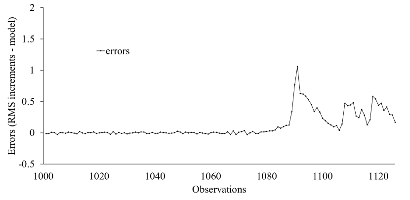
When bearings slide over a lubricated surface, vibrations are steady and predictable, in control. However, after a large period of utilization, microscopic fractures initiate a vicious cycle that increases vibrations exponentially until bearings fatigue and break. Quick detection of a sustained change in bearing vibrations creates an advantage that might allow preventive maintenance to avoid costly machine repairs. To illustrate the application of sequential normal scores on real measurements, the procedure was applied over a data set from the IEEE PHM 2012 Data Challenge organized by the IEEE Reliability Society and FEMTO-ST Institute. During the challenge to estimate the remaining useful life of bearings, several experiments to accelerate degradation were carried out on a laboratory experimental platform called PRONOSTIA. Datasets and further information about the data challenge are available in Nectoux et al. (2012). Vibrations were processed using a fast Fourier transform (FFT) and the results were summarized as RMS (root mean square) measurements, a convention used to to provide an indication of the amount of energy spent on vibration. FFT and RMS measurements were calculated by Barraza-Barraza (2015), where time series models are used to characterize PRONOSTIA’s bearing data. The specific data set used to create this example was taken from Nectoux et al. (2012), scenario 1, bearing 4. Here, the bearing was run to failure; hence, it is known, by design, that measurements describe a movement from an in-control state to an out-of-control state.

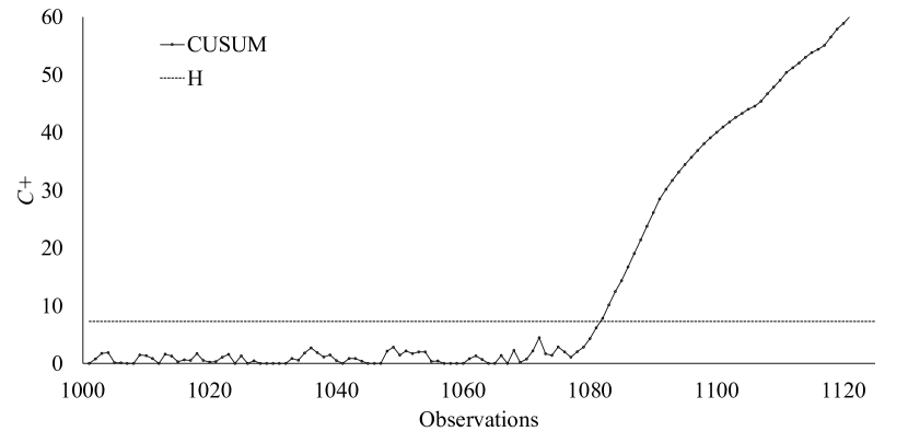
Using a least squares approach over the first 1000 RMS observations, an MA(1) was fitted over the first differences, and independent errors were used for process monitoring. A CUSUM chart was constructed after transforming the errors into sequential normal scores. Even if data is not normal, practitioners can rely on the normal approximation of the scores and proceed with a CUSUM chart set up for normally distributed observations. The monitored errors can be seen in Figure 1(a), and the corresponding CUSUM chart applied over the sequential normal scores is shown in Figure 1(b). A one-sided CUSUM for positive shifts with an allowance $k=0.25$ and a decision interval $H=7.267$ were used for monitoring to achieve an approximate in control $ARL$ of 500. A signal is triggered at observation 1082, just before vibrations start to exhibit an evident “violent” behavior.

(a) Monitored errors from bearing vibrations.

(b) One-sided CUSUM using sequential normal scores.

Figure 1: A CUSUM chart was used on sequential normal scores obtained from observed errors after fitting an ARIMA(0,1,1) model over a first set of 1000 in-control RMS vibration measurements from bearings at the IEEE PHM 2012 Data Challenge. A one-sided CUSUM with a reference value $k=0.25$ and a decision interval $H=7.267$ was used.

2.2 Batched observations with unknown quantiles

Let $\{X_{ij}:i=1,\ldots,;j=1,\ldots,m\}$ be a sequence of independent identically distributed random variables with continuous distribution function $F(x)$. The second subscript refers to the fact that these random variables are grouped into batches (samples) of size $m$. For the first batch ($i=1$) the $m$ random variables are ranked relative to the other random variables in that batch, and the ranks are denoted by $R_{1,j}$ for $j=1,\ldots,m$. For all subsequent batches the sequential rank $R_{i,j}$ of $X_{i,j}$, where $i$ stands for the batch number, and $i\geq 2$, is given by,

$$R_{i,j}(X_{i,j})=\sum_{k=1}^{i-1}\sum_{l=1}^{m}I(X_{k,l}\leq X_{i,j})+1$$ (2)

for $i\geq 2$ and $j=1,2,\ldots,m$, where $I(X_{kl}\leq X_{i,j})$ is an indicator function.

This sequential rank is computed for each $j=1,\ldots,m$ in batch $i$. Note that several of these sequential ranks within a batch may be equal to one another, but do not change as more batches are observed. Again, this can save considerable computing time when using rank-based nonparametric methods.

For reasons explained in Section 3 we will use

$$P_{1,j}=\frac{\left(R_{1,j}-0.5\right)}{m},$$ (3)

and

$$P_{i,j}=\frac{\left(R_{i,j}-0.5\right)}{m(i-1)+1}$$ (4)

for $i>1$, to estimate $F(X_{i,j})$. Sequential normal scores are obtained from $P_{i,j}$ using $Z_{i,j}=\Phi^{-1}\left(P_{i,j}\right)$ where $\Phi^{-1}$ stands for the inverse cumulative standard normal distribution function. As will be proven in Section 3, the sequence $\left\{Z_{i,j}:i=1,2,\ldots;j=1,2,\ldots,m\right\}$ consists of mutually independent asymptotically (as $i$ gets large) standard normal random variables. By comparing each random variable with only the previous batches plus itself, and not with other random variable in the same batch, the independence of the sequential ranks is kept, and the sensitivity to detect a change is improved by not using comparisons within a batch potentially from the alternative distribution.

2.2.1 Service time example

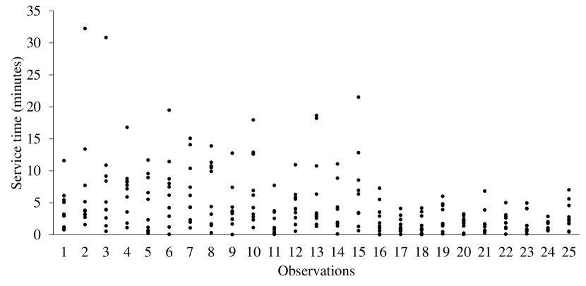
We use an example from Yang et al. (2012) and Yang and Arnold (2015) in which the efficiency of the service system in a bank is analyzed. The service process times for 10 counters were measured (in minutes) every 2 days for 30 days. Fifteen in-control samples of size $m=10$ were obtained from a bank branch. Yang and Arnold (2015) show that data appear to be right-skewed (see Figure 2(a)), hence a procedure based on the normal distribution is not recommended. Later, 10 new samples from a new automatic service system were collected. From the analysis carried out by Yang and Arnold (2015) there is indeed a change in the new samples. That is, the 10 new samples that belong to a out-of-control state showed a reduction in the variance. By performing a Phase I analysis, Yang and Arnold (2015) estimated the variance of the process from the first 15 samples, and carried a test on the remaining 10 samples. The test was rejected after the second sample.

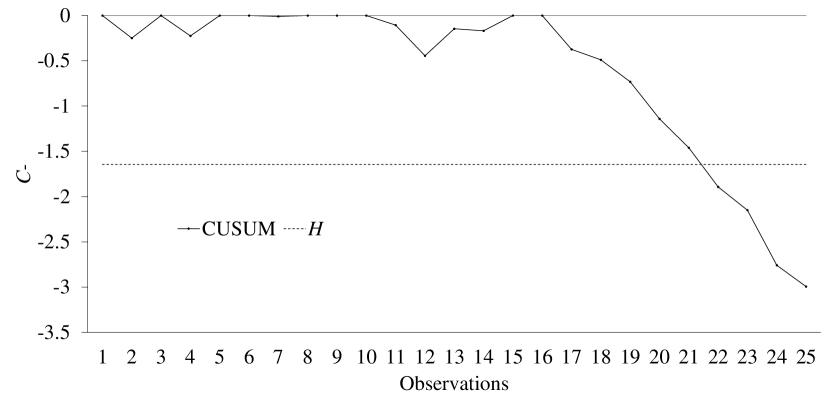
Without using a Phase I analysis to estimate an in-control value of the variance to use as reference, sequential normal scores can be adapted to test for a variance change. Scores $Z_{i,j}$ can be used in an optimal CUSUM for downward process variance by monitoring the statistic

$$C_{i}^{-}=min(0,C_{i-1}^{-}+s_{i}^{2}-k)$$

where $C_{0}=0$, $s_{i}^{2}$ corresponds to the sample variance (from the scores) in batch i, and

$$k=\frac{2\log(\frac{\sigma_{0}}{\sigma_{1}})\sigma_{0}^{2}\sigma_{1}^{2}}{\sigma_{1}^{2}-\sigma_{0}^{2}},$$

where $\sigma_{0}^{2}$ and $\sigma_{1}^{2}$ corresponds to the out-of-control and the in-control variance, respectively; which gives a signal when $C_{i}^{-}<H$. From Hawkins and Olwell (2012) we obtain a value of $H=-1.645$ and an allowance $k=0.793$ to achieve an $ARL_{0}$ of $370.0$, which is optimum for a variance reduction from 1 to 0.8. The value, 0.8, for the out-of-control variance was selected arbitrarily to illustrate the approach. Original observations and the results from the CUSUM are plotted in Figure 2. It can be seen that a variance reduction was signaled at observation 22, that is, 7 observations after the actual change. Note that the natural CUSUM change-point statistic, the greatest observation with cumulative value $C^{-}$ equal to zero, is 16, the actual first out-of-control sample. In this example, the first batch was transformed using their corresponding relative ranks, and the subsequent batches were ranked using sequential ranks. Then the inverse of a standard normal cumulative distribution was evaluated on the resulting $P_{i,j}$ as defined in equations (3) and (4).

If a priori information exists about the null distribution, such as the one obtained from a Phase I analysis as done in Yang and Arnold (2015), historical data, or a target median, an adaptation of the sequential normal scores to incorporate quantile information can be used to increase the efficiency of a test procedure. This adaptation is illustrated in the following two subsections.

(a) Original measurements from the Bank service times example.

(b) Optimal CUSUM for variance on sequential normal scores.

Figure 2: Optimal CUSUM chart for subgroup variance with k = 0.793 and H = -1.645 was used on sequential normal scores obtained from service times obtained from the bank example data set.

2.3 Individual observations with known quantile $\theta$

Let $X_{1},X_{2},\ldots,$ be a sequence of independent identically distributed random variables with a continuous distribution function $F(x)$. In contrast to Section 2.1 we will assume that a quantile $\theta$ and its corresponding probability $F(\theta)$ are known, or assumed to be known, such as $\theta$ = median. Define the conditional sequential rank $R_{i|\theta}$ of $X_{i}$ differently depending on if $X_{i}<\theta$ or if $X_{i}>\theta$. In particular, if $X_{i}<\theta$ then the conditional sequential rank $R_{i|\theta}$ of $X_{i}$ is the rank of $X_{i}$ relative only to the previous random variables that were less than $\theta$, including $X_{i}$. On the other hand, if $X_{i}>\theta$ then the conditional sequential rank $R_{i|\theta}$ of $X_{i}$ is the rank of $X_{i}$ relative only to the previous random variables that were greater than $\theta$, including $X_{i}$.

Let $N_{i}^{-}$ be the number of random variables, of the first $i$ random variables in the sequence, that are less than or equal to $\theta$, and let $N_{i}^{+}$ be the number of random variables, of the first $i$ random variables in the sequence that are greater than $\theta$. Then $N_{i}^{-}+N_{i}^{+}=i$. For reasons explained in Section 3 we will use

$$P_{i|\theta}=\begin{cases}F(\theta)\frac{R_{i|\theta}-0.5}{N_{i}^{-}}\quad&,if\quad X_{i}\leq\theta\\ F(\theta)+[1-F(\theta)]\frac{R_{i|\theta}-0.5}{N_{i}^{+}}\quad&,if\quad X_{i}>\theta\end{cases}.$$ (5)

to estimate $F(X_{i}|\theta)$. Conditional sequential normal scores are obtained from $P_{i|\theta}$ using $Z_{i|\theta}=\Phi^{-1}\left(P_{i|\theta}\right)$ where $\Phi^{-1}$ stands for the inverse cumulative standard normal distribution function. As will be proven in Section 3, the sequence $\left\{Z_{i|\theta}:i=1,2,...\right\}$ consists of mutually independent asymptotically (as $i$ gets large) standard normal random variables.

2.3.1 Concrete strength example

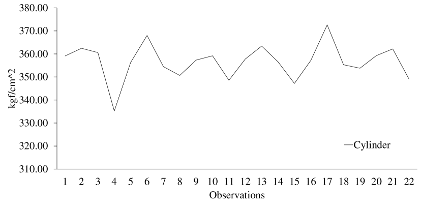
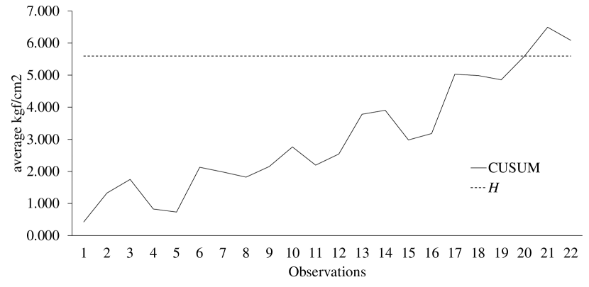
From Aichouni et al. (2014) we obtain a data set of compressive strength for ready mixed concrete. The compression strength of 22 samples of concrete with a target specification of 350 Kgf/cm² were measured over a period of 30 days. As shown by Aichouni et al., observations do not fit a normal distribution. They addressed the situation of non-normality by using a Johnson transformation. However, the use of a transformation in small data sets comes with the risk of over-fitting and the selection of a mistaken transformation function. By using conditional sequential normal scores, this risk is avoided. Nevertheless, Aichouni et al. did not evaluate whether sampled measurements achieved the target value, they tested only for isolated changes (where the parametric scenario might be the best approach). To continue with the analysis, we evaluate if the compressive strength is actually significantly larger than the median target. By defining the nominal value of 350 as the target process median, the analysis can be carried out by using conditional sequential normal scores from equation (5). Here, it is assumed that under the null distribution $F(350)=0.5$. Figure 3 shows the results after evaluating the conditional sequential normal scores with a CUSUM chart that assumes normal standard observations. From Qiu (2013), we obtained that an allowance of $k=0.25$ and a control limit $H=5.597$ used as parameters of a one-sided tabular CUSUM chart achieve an in-control performance of 200 in terms of average run length ($ARL_{0}$). Even though we are monitoring a null median of 350, and this information is incorporated into the sequential normal scores, the monitored scores still have a mean value of zero and their behavior can be approximated with a standard normal distribution. As can be seen, an alarm is signaled at sample 21, which indicates that the mixture is providing more strength than nominal specification. Because sequential normal scores provide a conservative approximation of the standard normal distribution, with a slightly smaller variance (see Subsection 3.2 for details), the true $ARL_{0}$ is at most the one specified by the CUSUM setup.

(a) Average compressive strength measurements.

(b) CUSUM chart on sequential normal scores.

Figure 3: CUSUM obtained from sequential normal scores of compressive strength for Ready Mixed Concrete (Kgf/cm²). The average was used as an individual observation. An allowance of $k=0.25$ and a decision interval of $H=5.597$ were used.

2.4 Batched observations with known quantile $\theta$

Let $\{X_{i,j}:i=1,\ldots,;j=1,\ldots,m\}$ be a sequence of independent identically distributed random variables with a continuous distribution function $F(x)$. The second subscript refers to the fact that these random variables are grouped into batches (samples) of size m. In contrast to Section 2.2 we will assume that a quantile $\theta$ and its corresponding probability $F(\theta)$ are known, or assumed to be known, such as $\theta$ = median. For the first batch ($i=1$) the random variables that are less than $\theta$ are ranked relative to only the other random variables in the first batch that are less than $\theta$, and the ranks of the random variables that are greater than $\theta$ are ranked relative to only the other random variables in the first batch that are greater than $\theta$. These conditional ranks are denoted by $R_{1,j|\theta}$ for $j=1,\ldots,m$. For all subsequent batches define the conditional sequential rank $R_{i,j|\theta}$ of $X_{i,j}$ differently depending on if $X_{i,j}\leq\theta$ or if $X_{i,j}>\theta$ . In particular, if $X_{i,j}\leq\theta$, then the conditional sequential rank $R_{i,j|\theta}$ of $X_{i,j}$ is the rank of $X_{i,j}$ relative to only the random variables that were less than $\theta$ in the previous batches, including $X_{i,j}$, but no other random variables in the same batch i. On the other hand, if $X_{i,j}>\theta$ then the conditional sequential rank $R_{i,j|\theta}$ of $X_{i,j}$ is the rank of $X_{i,j}$ relative to only the previous random variables that were greater than $\theta$ in the previous batches, including $X_{i,j}$ but no other random variables from the same batch i.

Let $N_{1}^{-}$ be the number of random variables of the first batch in the sequence, that are less or equal than $\theta$ and $N_{1}^{+}$ be the number of random variables of the first batch that are greater than $\theta$. For $i>1$, let $N_{i}^{-}$ be the number of random variables, of the first $i-1$ batches of random variables in the sequence, that are less than $\theta$, and let $N_{i}^{+}$ be the number of random variables of the first $i-1$ batches of random variables in the sequence that are greater than $\theta$. Then, $N_{1}^{-}+N_{1}^{+}=m$ and $N_{i}^{-}+N_{i}^{+}=(i-1)m$ for $i>1$. For reasons explained in Section 3 we will use $P_{1,j|\theta}$ for $i=1$ and $P_{i,j|\theta}$ for $i>1$, as

$$P_{1,j|\theta}=\begin{cases}F(\theta)\frac{R_{1,j|\theta}-0.5}{N_{1}^{-}}\quad&,\quad X_{1,j}\leq\theta\\ F(\theta)+(1-F(\theta))\frac{R_{1,j|\theta}-0.5}{N_{1}^{+}}\quad&,\quad X_{1,j}>\theta\end{cases},$$ (6)

and for $i\geq 2$

$$P_{i,j|\theta}=\begin{cases}F(\theta)\frac{R_{i,j|\theta}-0.5}{N_{i}^{-}+1}\quad&,\quad X_{i,j}\leq\theta\\ F(\theta)+(1-F(\theta))\frac{R_{i,j|\theta}-0.5}{N_{i}^{+}+1}\quad&,\quad X_{i,j}>\theta\end{cases}.$$ (7)

Conditional sequential normal scores are obtained from $P_{i,j|\theta}$ using $Z_{i,j|\theta}=\Phi^{-1}\left(P_{i,j|\theta}\right)$ where $\Phi^{-1}$ stands for the inverse cumulative standard normal distribution function. As proven in Section 3, the sequence $\left\{Z_{i,j|\theta}:i\geq 2;j=1,\ldots,m\right\}$ consists of mutually independent asymptotically (as $i$ gets large) standard normal random variables.

2.4.1 GPA example

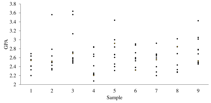
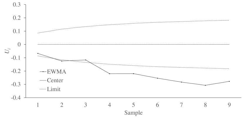
From Bakir and McNeal (2010) we obtained data that consists of GPA results from management major students of the Department of Business Administration at Alabama State University. Measurements were taken from the period of Spring 2005 through Spring 2009. The research showed that GPAs maintained a desired target median level of 2.600 but they were significantly below the higher target median of 2.800, which represented 70% of the maximum score of 4 points. The data presented problems of satisfying the assumption of normality, and a nonparametric control chart based on signed ranks was proposed by the authors. The original data is plotted in Figure 4(a). Using equation (6) and (7), observations are transformed into conditional sequential normal scores that, in turn, are evaluated using an EWMA statistic

$$U_{i}=\lambda\bar{Z_{i}}+(1-\lambda)U_{i-1}$$ (8)

where $U_{0}=0$, and $\bar{Z_{i}}$ is the average of $Z_{i,j|\theta}$; $j=1,\ldots,m$; as seen in Qiu (2013). Significance is achieved when the plotted statistic surpasses the limits

$$\pm\rho\sqrt{\frac{\lambda}{2-\lambda}[1-(1-\lambda)^{2i}]}\frac{\sigma}{\sqrt{m}}.$$ (9)

Here, $\sigma=1$, the variance of the standard normal distribution approximated by the sequential normal scores. Following the spc package in R, the xewma.arl function is used in a calibration process to obtain the value of parameter $\rho=2.714$ with a convenient $\lambda=0.1$ that approximate a zero-start $ARL_{0}\approx 370.0$ with variable control limits. Results, as seen in Figure 4(b), show a significant difference between observed data and the target value of 2.8. Even though the original analysis evaluated batches individually, results are consistent with the overall analysis, as a signal is triggered first at the second sample and continues after the fourth.

(a) Original GPA measurements.
 

(b) EWMA for subgroup observations on sequential normal scores.

Figure 4: EWMA control chart applied over sequential normal scores from the GPA data set example with a null median of 2.8.

2.5 Application remarks

Sequential normal scores extend the use of parametric procedures to deal with observations from an unknown distribution. However, practitioners should be aware that such a transformation is only appropriate to deal with sustained changes. If isolated changes are a concern, as might be the case for a test for outliers, a parametric approach might be the best option.

Big data users and researchers might find the sequential normal scores transformation appealing due to its asymptotic behavior and the reduced computational effort required for its implementation. On one hand, as seen in Section 3, the transformation becomes close to an exact quantile transformation into normality. When a large data set is available, model based approaches usually fail to fit the precise observed behavior. Nonparametric approaches, such as sequential normal scores, are more likely to provide null distributions with a better fit to the true unknown probability law behind the statistic used to evaluate the data. On the other hand, by following a sequential ranking scheme that avoids re-ranking previous observation, a large amount of computational time is saved. For instance, Figure 5, illustrates the time, in seconds, it takes for three nonparametric statistics used in statistical process control literature, including sequential normal scores, to be calculated once, after a number of observations is available from a data stream. We considered the statistic of Hawkins and Deng (2010), which is a change-point statistic based on Mann-Whitney statistic; and the statistic of Chowdhury et al. (2015), where a reference sample is evaluated against a monitored sample using the Lepage statistic. All measurements were carried using a Hewlett-Packard PC, model 6200 PRO SFF with an Intel Core I3 2120 processor, 500GB of hard drive, 3GB for memory and Windows 7 Pro. It can be seen that the statistic of Hawkins and Deng (2010) could not be computed for sample size bigger than $10^{4}$, whereas the statistic of Chowdhury et al. (2015) and sequential normal score statistic presented good performance in terms of computational time for data streams until $10^{7}$. In each scenario the computational time of sequential normal scores is at least 10 times faster than Chowdhury et al.’s [2015] statistic.

Figure 5: Computer times to compute a charting statistic over different number of observations from Hawkins and Deng (2010) (CC-MW), Chowdhury et al. (2015) (Lepage), and the sequential normal scores (SNS).

3 Theoretical framework

3.1 The mean of sequential normal scores

Consider a sequence $X_{1},X_{2},...,$ of independent random variables identically distributed according to a continuous distribution function $F(x)$. Note that $F(X_{i})$ is a uniform $(0,1)$ random variable for all $i\geq 1$. Sequential ranks $R_{i}=R(X_{i})$ are defined by Parent (1965) as $R_{1}=1$ and, for $i\geq 2$ as

$$R_{i}=\sum_{j=1}^{i-1}I(X_{j}\leq X_{i})+1.$$ (10)

Note that the indicator variables $I(X_{j}\leq X_{i})$ are Bernoulli random variables for $1\leq j\leq i-1$, with mean $1/2$, variance $1/4$, and covariance $1/12$.

Consider $P_{i}=P(X_{i})$ as an estimator of $F(X_{i})$, where

$$P_{i}=\frac{(R_{i}-1+a)}{i-1+b}\quad ,\quad b>0;\quad 0<a<b.$$ (11)

Thus, $0<P_{i}<1$ and the sequential normal score $Z_{i}=\Phi^{-1}(P_{i})$ is a well-defined normal score, where $\Phi^{-1}$ is the inverse of the standard normal distribution function

We would like to choose $a$ and $b$ so that the mean and variance of $Z_{i}$ are 0 and 1 respectively. The mean of $Z_{i}$ equals 0 if and only if the mean (and median) of $P_{i}$ is 0.5, due to the quantile preserving property of monotonic transformations. The mean of $P_{i}$ is, from equation (10)

$$E(P_{i})=\frac{\frac{i-1}{2}+a}{i-1+b}$$ (12)

which equals 0.5 if and only if $b=2a$. The variance of $Z_{i}$ is a function of $b$, which is discussed in next subsection.

3.2 The variance of sequential normal scores

The variance of $P_{i}$ can be easily found to be

$$Var(P_{i})=\frac{\frac{i-1}{4}+\frac{(i-1)(i-2)}{12}}{(i-1+b)^{2}}=\frac{i^{2}-1}{12(i-1+b)^{2}}$$ (13)

which is a function of b, and equals 1/12 (the variance of $F(X)$) if and only if $b=1-i+\sqrt{i^{2}-1}$. As $i$ gets large, $b$ approaches 1, which suggests using $b=1$ for finite sample sizes.

Unfortunately the variance is not preserved in the normal scores transformation, so we are forced to use numerical approximation methods to find values of b that result in $Var(Z_{i})=1$. These results are summarized in Table 1.

Table 1 shows that the actual value of $b$ to obtain $Var(Z_{i})=1$ increases from $b=0.465$ for $i=2$ to $b=0.915$ for $i=5000$. The effect of using $b=1$ as an approximation is slight (less than $2\%$ error for the standard deviation of $Z_{i}$) for $i>31$, and the approximation

$$b=0.824-\frac{0.792}{i}$$ (14)

results in less than a $1\%$ error for $i>2$ ($3.7\%$ error for $i=2$ ). If $b=1$ is used for all values the result is a conservative estimate for the standard deviation of the sequential normal scores $Z_{i}$, so that is what we used in our examples. A slight increase in power results from using the approximation for $b$ when $i<31$. Nevertheless, the increased power was not big enough to change the decisions obtained from the particular numerical examples shown in Section 2.

This approximation problem has been previously addressed. For example, Van der Waerden (1952) used $a=1$, $b=2$; Blom (1954) used $a=5/8$, $b=1.25$; Tukey (1962) used $a=2/3$, $b=4/3$; and Bliss et al. (1956) used $a=1/2$, $b=1$ which they called a “rankit”. An empirical study by Solomon and Sawilowsky (2009) compared these four approximations and concluded that “Rankit emerged as the most accurate method among all sample sizes and distributions, thus it should be the default selection for score normalization in the social and behavioral sciences”(p.448). Note that all four approximations preserve a mean of 0 for the normal scores because $b=2a$. However all four approximations result in a variance less than 1.0 which we addressed in this section.

Table 1: Standard deviation of $Z_{i}$ when $b=1$, and values of $b$ that give 1.0 for the standard deviation of $Z_{i}$. Also given is the standard deviation of $Z_{i}$ when the approximation for $b$ from equation (14) is used.

i	$\sigma$ when $b=1$	Value of $b$ to obtain $\sigma=1$	Value of $b$ using approximation	Value of $\sigma$ using $b$ from equation (14)
2	.675	.465	.428	1.037
3	.790	.565	.560	1.004
4	.844	.618	.626	.996
5	.876	.652	.666	.994
10	.938	.727	.745	.995
20	.969	.778	.784	.999
30	.979	.800	.798	1.000
31	.980	.802	.798	1.000
32	.980	.803	.799	1.000
100	.994	.847	.816	1.001
1000	.999	.896	.823	1.001
5000	1.000	.915	.824	1.000

3.3 Include a priori information about a known quantile

Let $X_{1},X_{2},\ldots,$ be a sequence of independent observations, and $F(\cdot)$ corresponds to their common cumulative null distribution. Also, assume that $F(\theta)$ and $\theta$ are known, where the latter is a constant. (To facilitate notation we’ll be using $F(a)$ and $P(X\leq a)$, without the subindex in the variable $X$, interchangeably, to express the evaluation of the cumulative distribution function at a constant a under the null hypothesis, and we will suppress the fact that $F(\theta)$ is known even though it is implicit in all of the probabilities of this section).

Given a constant $a$, a conditional sequential normal scores statistic can be constructed by noting that

$$P(X\leq a)=P(X\leq a|X\leq\theta)P(X\leq\theta)+P(X\leq a|X>\theta)P(X>\theta)$$ (15)

where the $P(X\leq a)$ can be estimated by using

$$\hat{P}(X_{i}\leq a|X_{i}\leq\theta)=\frac{\sum_{j=1}^{i-1}I(X_{j}\leq a)I(X_{j}\leq\theta)+0.5}{\sum_{j=1}^{i-1}I(X_{j}\leq\theta)+1},$$ (16)

and

$$\hat{P}(X_{i}\leq a|X_{i}>\theta)=\frac{\sum_{j=1}^{i-1}I(X_{j}\leq a)I(X_{j}>\theta)+0.5}{\sum_{j=1}^{i-1}I(X_{j}>\theta)+1}$$ (17)

in equation (15). Equations (16) and (17) are maximum likelihood estimators with biasing constants 0.5 and 1 defined in previous section. Hence, using the fact that $P(X\leq\theta)$ is known, a cumulative probability can be better estimated by

$$\hat{P}(X\leq X_{i})=\begin{cases}P(X\leq\theta)\frac{\sum_{j=1}^{i-1}I(X_{j}\leq X_{i})I(X_{j}\leq\theta)+0.5}{\sum_{j=1}^{i-1}I(X_{j}\leq\theta)+1}\quad&,\quad X_{i}\leq\theta\\ P(X\leq\theta)+P(X>\theta)\frac{\sum_{j=1}^{i-1}I(X_{j}\leq X_{i})I(X_{j}>\theta)+0.5}{\sum_{j=1}^{i-1}I(X_{j}>\theta)+1}\quad&,\quad X_{i}>\theta\end{cases}$$ (18)

Hence, conditional sequential normal scores are then defined by evaluating $\Phi^{-1}(\hat{P}(X\leq X_{i}))$.

3.4 Sequence of Independent Statistics

The following Proposition states the independence of the sequence $\left\{P_{i}:1,\ldots,n\right\}$ and the asymptotic distribution of the sequence $\left\{Z_{i}:1,\ldots,n\right\}$, of model in Section 2.1.

Proposition.

Let $X_{1},X_{2},...,X_{n}$ be a sequence of i.i.d. random variables. Define $P_{i}$ and $Z_{i}$ as in Section 2.1. Then,

1. Series $\left\{P_{i}:1,\ldots,n\right\}$ are mutually independent random variables.

2. $\left\{Z_{i}:1,\ldots,n\right\}$ are independent asymptotically standard normal random variables.

Proof.

Since Theorem 1.1 in Barndorff-Nielsen (1963) states that the sequence of random variables $\left\{R_{i}(X_{i}):i=1,2,\ldots\right\}$ are mutually independent, it follows by Theorem 4.6.12 in Casella and Berger (2002) that $\left\{P_{i}:i=1,2,\ldots\right\}$ are also mutually independent random variables. This in turn implies that the $Z_{i}$ are also mutually independent. By applying the Strong Law of Large Numbers, the Glivenko-Cantelli Theorem implies that $P_{i}$ converges uniformly to a uniform (0,1) random variable, and thus $Z_{i}$ converges to a standard normal random variable, as $i$ goes to infinity. ∎

It can be noted that the results of the Proposition apply to the models in Sections 2.2, 2.3 and 2.4 as well. The variations in the proof involve redefining sequential ranks in each section, but otherwise are trivial and are omitted here.

Corollary.

The results of the Proposition hold even if Pi,j is given by equations (3) and (4) in Section 2.2, or if $P_{i|\theta}$ is given by equation (5) in Section 2.3, or if $P_{ij|\theta}$ is given by equations (6) and (7) in Section 2.4.

4 Limited sample approximation

Previous results indicate that sequential normal scores are independent, and they approach to a standard normal random variable as the series grows to infinity. However, in practice, practitioners are limited to a finite number of observations and might wonder how sequential normal scores will perform with that restriction. Because this paper introduces the concept of sequential normal scores for the first time, the authors thought it would be beneficial to examine the behavior of sequential normal scores in more detail. Extensive Monte Carlo simulations were conducted to determine how well a standard normal distribution approximates the exact distribution of sequential normal scores, as defined in Section 2.1. Although an exact distribution can be obtained by using the fact that every ordering of the usual ranks of a random sequence of independent and identically distributed random variables is equally likely, and there is a one-to-one correspondence between the usual ranks and the sequential ranks, it was more convenient to use Monte Carlo sampling in this study.

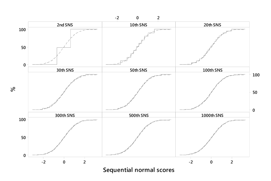
First, the exact distribution of the $n$-th sequential rank $R_{n}$ is well known to be the uniform distribution over the integers 1 to $n$. But, after converting to $P_{n}$ and then to $Z_{n}$, how does the distribution of $Z_{n}$ compare with the standard normal distribution? Figure 6 shows the comparison for various values of $n$ from 2 to 1000. It shows that the choice of using $b=1$ for all values of $n$ does not appear to make an appreciable difference, as opposed to tailoring values of $b$ to make the variance closer to 1.0.

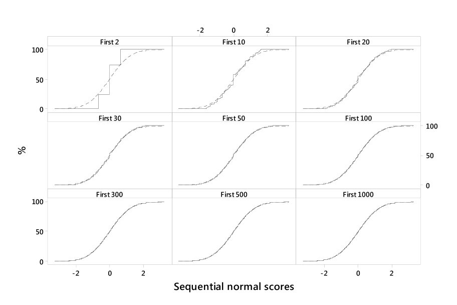
Second, the empirical distribution of the first $n$ sequential normal scores is compared with the standard normal distribution by averaging 1000 empirical distribution functions, with the results shown in Figure 7. These results show that the standard normal quantiles in the tails tend to be larger (in absolute value) than the exact quantiles, which will result in conservative tests, but the difference appears to be negligible for $n$ greater than 30. This agrees with our comparison of exact variances with the variance of the standard normal distribution in Section 3.2. Also, these exact distributions reveal a relatively large probability at $x=0$, but this jump disappears almost completely as $n$ reaches 100 or more.

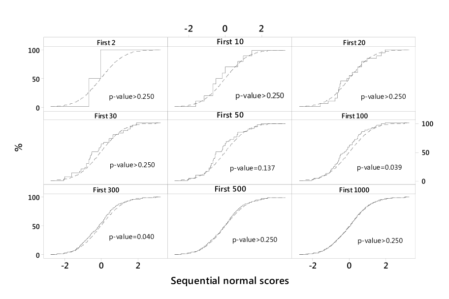
Finally, a single random sequence is evaluated at various lengths in Figure 8, and an Anderson-Darling goodness of fit is applied. The resulting empirical distribution functions show some divergence from the standard normal distribution in the middle values of $x$, but good agreement in the tails of the distributions where a good approximation is more important. The resulting p-values for this series are significant at $n=100$ and $n=300$, but the significance disappears for larger values of $n$.

Figure 6: The exact distribution (solid line) of the $n$-th sequential normal score at different values of $n$, and the cumulative standard normal distribution (dotted line).

Figure 7: The expected value of the empirical distribution function (solid line) for different sequence lengths $n$, and the cumulative standard normal distribution (dotted line).

Figure 8: Empirical distributions of a sample path of sequential normal scores, the cumulative normal standard distribution and the p-value obtained from an Anderson-Darling test for $N(0,1)$ at different moments in time.

5 Conclusions

A new sequential statistic based on normal scores, named sequential normal scores, was proposed as a link between parametric and nonparametric procedures that are sequential in nature, such as control charts used in online monitoring of data streams. The statistic extends the concept of sequential ranks into a modified version of normal scores to obtain a sequence of asymptotically standard normal and independent scores that can be analyzed with existing procedures originally created to deal with normal and independent observations. Four different versions of the statistic were presented to address different situations with individual or batched observations, or when a priori knowledge about a quantile exists or not. When sustained changes are a concern, the applicability of the proposed transformation is illustrated with the utilization of control chart on sequential normal scores from different databases available in the open literature. It is shown that sequential normal scores used with control charts are capable of detecting changes in a process, requiring only i.i.d. observations under the null hypothesis. Also, if a priori knowledge exists about a process quantile under the null assumption, which might be the case when it is desired that a process follows a target median, sequential normal scores are adapted to incorporate existing information in such a way that control charts with sequential normal scores become sensitive to detect changes at the very start of a monitoring. Big data users might be willing to analyze their data streams with the sequential normal scores transformation. If streams are very large, the fit to a normal distribution provided by sequential normal scores might be, in many cases, arguably better, than the fit one might find from parametric models–unless the true underlying distribution is known. In addition, even though the sequential normal scores lack of complexity makes them “computer friendly”, if data streams are very large, it is easy to restrict our comparisons to a moving window of reasonable size (e.g. 1000 or 5000) when determining the sequential ranks. This sets the memory usage of a computer and the number of operations to transform data constant. The proposed statistic offers a tool that makes nonparametric analysis readily available for practitioners and an approach that can be used by researchers to deal with new problems as they become available.

References

- Aichouni et al. [2014] M Aichouni, AI Al-Ghonamy, and L Bachioua. Control charts for non-normal data: Illustrative example from the construction industry business. In Proceedings of the 16th International Conference on Mathematical and Computational Methods in Science and Engineering, 24, pages 71–76, Kuala Lumpur, Malaysia, 2014. WSEAS Press.
- Bakir and McNeal [2010] Saad T Bakir and Bob McNeal. Monitoring the level of students’ gpas over time. American Journal of Business Education (AJBE), 3(6):43–50, 2010.
- Barndorff-Nielsen [1963] Ole Barndorff-Nielsen. On the limit behaviour of extreme order statistics. The Annals of Mathematical Statistics, 34(3):992–1002, 1963.
- Barraza-Barraza [2015] Diana Barraza-Barraza. An adaptive ARX model to Estimate an Asset Remaining Useful Life. PhD thesis, Texas Tech University, 2015.
- Bliss et al. [1956] CI Bliss, Mary L Greenwood, and Edna Sakamoto White. A rankit analysis of paired comparisons for measuring the effect of sprays on flavor. Biometrics, 12(4):381–403, 1956.
- Blom [1954] Gunnar Blom. Transformations of the binomial, negative binomial, poisson and 2 distributions. Biometrika, 41(3/4):302–316, 1954.
- Box [1957] George EP Box. Evolutionary operation: A method for increasing industrial productivity. Applied Statistics, pages 81–101, 1957.
- Casella and Berger [2002] George Casella and Roger L Berger. Statistical inference, volume 2. Duxbury Pacific Grove, CA, 2002.
- Chowdhury et al. [2015] Shovan Chowdhury, Amitava Mukherjee, and Subhabrata Chakraborti. Distribution-free phase ii cusum control chart for joint monitoring of location and scale. Quality and Reliability Engineering International, 31(1):135–151, 2015.
- Dodge and Romig [1929] Harold French Dodge and HG Romig. A method of sampling inspection. Bell System Technical Journal, 8(4):613–631, 1929.
- Hawkins and Deng [2010] Douglas M Hawkins and Qiqi Deng. A nonparametric change-point control chart. Journal of Quality Technology, 42(2):165, 2010.
- Hawkins and Olwell [2012] Douglas M Hawkins and David H Olwell. Cumulative sum charts and charting for quality improvement. Springer Science & Business Media, 2012.
- Nectoux et al. [2012] Patrick Nectoux, Rafael Gouriveau, Kamal Medjaher, Emmanuel Ramasso, Brigitte Chebel-Morello, Noureddine Zerhouni, and Christophe Varnier. Pronostia: An experimental platform for bearings accelerated degradation tests. In IEEE International Conference on Prognostics and Health Management, PHM’12., pages 1–8. IEEE Catalog Number: CPF12PHM-CDR, 2012.
- Parent [1965] E.A. Parent. Sequential Ranking Procedures. PhD thesis, Department of Statistics, Stanford University., 1965. URL https://books.google.com.mx/books?id=pYFCAAAAIAAJ.
- Qiu [2013] Peihua Qiu. Introduction to statistical process control. CRC Press, 2013.
- Reynolds [1975] Marion R Reynolds. A sequential signed-rank test for symmetry. The Annals of Statistics, 3:382–400, 1975.
- Ross et al. [2011] Gordon J Ross, Dimitris K Tasoulis, and Niall M Adams. Nonparametric monitoring of data streams for changes in location and scale. Technometrics, 53(4):379–389, 2011.
- Shewhart [1931] Walter A. Shewhart. Economic control of quality of manufactured product. D. Van Nostrand Company, Inc., 1931.
- Solomon and Sawilowsky [2009] Shira R Solomon and Shlomo S Sawilowsky. Impact of rank-based normalizing transformations on the accuracy of test scores. Journal of Modern Applied Statistical Methods, 8(2):448–462, 2009.
- Tukey [1962] John W Tukey. The future of data analysis. The Annals of Mathematical Statistics, 33(1):1–67, 1962.
- Van der Waerden [1952] BL Van der Waerden. Order tests for the two-sample problem and their power. In Indagationes Mathematicae (Proceedings), volume 55, pages 453–458. Elsevier, 1952.
- Wald [1945] Abraham Wald. Sequential tests of statistical hypotheses. The Annals of Mathematical Statistics, 16(2):117–186, 1945.
- Wald and Wolfowitz [1948] Abraham Wald and Jacob Wolfowitz. Optimum character of the sequential probability ratio test. The Annals of Mathematical Statistics, 19:326–339, 1948.
- Yang and Arnold [2015] Su-Fen Yang and Barry C Arnold. A new approach for monitoring process variance. Journal of Statistical Computation and Simulation, pages 1–17, 2015.
- Yang et al. [2012] Su-Fen Yang, Tsung-Chi Cheng, Ying-Chao Hung, and Smiley W Cheng. A new chart for monitoring service process mean. Quality and Reliability Engineering International, 28(4):377–386, 2012.