Frequentist Consistency
of Variational Bayes

Abstract

A key challenge for modern Bayesian statistics is how to perform scalable inference of posterior distributions. To address this challenge, variational Bayes (vb) methods have emerged as a popular alternative to the classical Markov chain Monte Carlo (mcmc) methods. vb methods tend to be faster while achieving comparable predictive performance. However, there are few theoretical results around vb. In this paper, we establish frequentist consistency and asymptotic normality of vb methods. Specifically, we connect vb methods to point estimates based on variational approximations, called frequentist variational approximations, and we use the connection to prove a variational Bernstein–von Mises theorem. The theorem leverages the theoretical characterizations of frequentist variational approximations to understand asymptotic properties of vb. In summary, we prove that (1) the vb posterior converges to the Kullback-Leibler (kl) minimizer of a normal distribution, centered at the truth and (2) the corresponding variational expectation of the parameter is consistent and asymptotically normal. As applications of the theorem, we derive asymptotic properties of vb posteriors in Bayesian mixture models, Bayesian generalized linear mixed models, and Bayesian stochastic block models. We conduct a simulation study to illustrate these theoretical results.

Keywords: Bernstein–von Mises, Bayesian inference, variational methods, consistency, asymptotic normality, statistical computing

1 Introduction

Bayesian modeling is a powerful approach for discovering hidden patterns in data. We begin by setting up a probability model of latent variables and observations. We incorporate prior knowledge by setting priors on latent variables and a functional form of the likelihood. Finally we infer the posterior, the conditional distribution of the latent variables given the observations.

For many modern Bayesian models, exact computation of the posterior is intractable and statisticians must resort to approximate posterior inference. For decades, Markov chain Monte Carlo (mcmc) sampling (Hastings:1970; gelfand1990sampling; Robert:2004) has maintained its status as the dominant approach to this problem. mcmc algorithms are easy to use and theoretically sound. In recent years, however, data sizes have soared. This challenges mcmc methods, for which convergence can be slow, and calls upon scalable alternatives. One popular class of alternatives is variational Bayes (vb) methods.

To describe vb, we introduce notation for the posterior inference problem. Consider observations $x=x_{1:n}$. We posit local latent variables $z=z_{1:n}$, one per observation, and global latent variables $\theta=\theta_{1:d}$. This gives a joint,

$$p(\theta,x,z)=p(\theta)\prod_{i=1}^{n}p(z_{i}\,|\,\theta)p(x_{i}\,|\,z_{i},\theta).$$ (1)

The posterior inference problem is to calculate the posterior $p(\theta,z\,|\,x)$.

This division of latent variables is common in modern Bayesian statistics. In the Bayesian Gaussian mixture model (gmm) (roberts1998bayesian), the component means, covariances, and mixture proportions are global latent variables; the mixture assignments of each observation are local latent variables. In the Bayesian generalized linear mixed model (glmm) (breslow1993approximate), the intercept and slope are global latent variables; the group-specific random effects are local latent variables. In the Bayesian stochastic block model (sbm) (Wiggins:2008), the cluster assignment probabilities and edge probabilities matrix are two sets of global latent variables; the node-specific cluster assignments are local latent variables. In the latent Dirichlet allocation (lda) model  (blei2003latent), the topic-specific word distributions are global latent variables; the document-specific topic distributions are local latent variables. We will study all these examples below.

vb methods formulate posterior inference as an optimization (jordan1999introduction; wainwright2008graphical; Blei:2016). We consider a family of distributions of the latent variables and then find the member of that family that is closest to the posterior.

Here we focus on mean-field variational inference (though our results apply more widely). First, we posit a family of factorizable probability distributions on latent variables

$$\mathcal{Q}^{n+d}=\left\{q:q(\theta,z)=\textstyle\prod^{d}_{i=1}q_{\theta_{i}}(\theta_{i})\prod_{j=1}^{n}q_{z_{j}}(z_{j})\right\}.$$

This family is called the mean-field family. It represents a joint of the latent variables with $n+d$ (parametric) marginal distributions, $\{q_{\theta_{1}},\ldots,q_{\theta_{d}},q_{z_{1}},\ldots,q_{z_{n}}\}$.

vb finds the member of the family closest to the exact posterior $p(\theta,z\,|\,x)$, where closeness is measured by kl divergence. Thus vb seeks to solve the optimization,

$$q^{*}(\theta,z)=\operatorname*{arg\,min}_{q(\theta,z)\in\mathcal{Q}^{n+d}}\lx@glossaries@gls@link{acronym}{KL}{\leavevmode\textsc{kl}}(q(\theta,z)\,||\,p(\theta,z\leavevmode\nobreak\ |\leavevmode\nobreak\ x)).$$ (2)

In practice, vb finds $q^{*}(\theta,z)$ by optimizing an alternative objective, the evidence lower bound (elbo),

$$\lx@glossaries@gls@link{acronym}{ELBO}{\leavevmode\textsc{elbo}}(q(\theta,z))=-\int q(\theta,z)\log\frac{q(\theta,z)}{p(\theta,x,z)}\text{d}\theta\text{d}z.$$ (3)

This objective is called the elbo because it is a lower bound on the evidence $\log p(x)$. More importantly, the elbo is equal to the negative KL plus $\log p(x)$, which does not depend on $q(\cdot)$. Maximizing the elbo minimizes the kl (jordan1999introduction).

The optimum $q^{*}(\theta,z)=q^{*}(\theta)q^{*}(z)$ approximates the posterior, and we call it the vb posterior. Though it cannot capture posterior dependence across latent variables, it has hope to capture each of their marginals. In particular, this paper is about the theoretical properties of the vb posterior $q^{*}(\theta)$, the vb posterior of $\theta$. We will also focus on the corresponding expectation of the global variable, i.e., an estimate of the parameter. It is

$$\hat{\theta}^{*}_{n}:=\int\theta\cdot q^{*}(\theta)\text{d}\theta.$$

We call $\theta^{*}$ the variational Bayes estimate (vbe).

vb methods are fast and yield good predictive performance in empirical experiments (Blei:2016). However, there are few rigorous theoretical results. In this paper, we prove that (1) the vb posterior converges in total variation (tv) distance to the kl minimizer of a normal distribution centered at the truth and (2) the vbe is consistent and asymptotically normal.

These theorems are frequentist in the sense that we assume the data come from $p(x,z\,;\,\theta_{0})$ with a true (nonrandom) $\theta_{0}$. We then study properties of the corresponding posterior distribution $p(\theta\,|\,x)$, when approximating it with variational inference. What this work shows is that the vb posterior is consistent even though the mean field approximating family can be a brutal approximation. In this sense, vb is a theoretically sound approximate inference procedure.

1.1 Main ideas

We describe the results of the paper. Along the way, we will need to define some terms: the variational frequentist estimate (vfe), the variational log likelihood, the vb posterior, the vbe, and the vb ideal. Our results center around the vb posterior and the vbe. (Table 1 contains a glossary of terms.)

The variational frequentist estimate (vfe) and the variational log likelihood.  The first idea that we define is the variational frequentist estimate (vfe). It is a point estimate of $\theta$ that maximizes a local variational objective with respect to an optimal variational distribution of the local variables. (The vfe treats the variable $\theta$ as a parameter rather than a random variable.) We call the objective the variational log likelihood,

$$M_{n}(\theta\,;\,x)=\max_{q(z)}\,\,\mathbb{E}_{q(z)}\left[\log p(x,z\,|\,\theta)-\log q(z)\right].$$ (4)

In this objective, the optimal variational distribution $q^{\dagger}(z)$ solves the local variational inference problem,

$$q^{\dagger}(z)=\arg\min_{q}\,\textrm{KL}(q(z)\,||\,p(z\,|\,x,\theta)).$$ (5)

Note that $q^{\dagger}(z)$ implicitly depends on both the data $x$ and the parameter $\theta$.

With the objective defined, the vfe is

$$\hat{\theta}_{n}=\arg\max_{\theta}\,M_{n}(\theta\,;\,x).$$ (6)

It is usually calculated with variational expectation maximization (em) (wainwright2008graphical; ormerod2010explaining), which iterates between the E step of Equation 5 and the M step of Equation 6. Recent research has explored the theoretical properties of the vfe for stochastic block models (bickel2013asymptotic), generalized linear mixed models (hall2011asymptotic), and Gaussian mixture models (westling2015establishing).

We make two remarks. First, the maximizing variational distribution $q^{\dagger}(z)$ of Equation 5 is different from $q^{*}(z)$ in the vb posterior: $q^{\dagger}(z)$ is implicitly a function of individual values of $\theta$, while $q^{*}(z)$ is implicitly a function of the variational distributions $q(\theta)$. Second, the variational log likelihood in Equation 4 is similar to the original objective function for the em algorithm (Dempster:1977). The difference is that the em objective is an expectation with respect to the exact conditional $p(z\,|\,x)$, whereas the variational log likelihood uses a variational distribution $q(z)$.

Variational Bayes and ideal variational Bayes.  While earlier applications of variational inference appealed to variational em and the vfe, most modern applications do not. Rather they use vb, as we described above, where there is a prior on $\theta$ and we approximate its posterior with a global variational distribution $q(\theta)$. One advantage of vb is that it provides regularization through the prior. Another is that it requires only one type of optimization: the same considerations around updating the local variational factors $q(z)$ are also at play when updating the global factor $q(\theta)$.

To develop theoretical properties of vb, we connect the vb posterior to the variational log likelihood; this is a stepping stone to the final analysis. In particular, we define the vb ideal posterior $\pi^{*}(\theta\,|\,x)$,

$$\pi^{*}(\theta\,|\,x)=\frac{p(\theta)\exp\{M_{n}(\theta\,;\,x)\}}{\int p(\theta)\exp\{M_{n}(\theta\,;\,x)\}\text{d}\theta}.$$ (7)

Here the local latent variables $z$ are constrained under the variational family but the global latent variables $\theta$ are not. Note that because it depends on the variational log likelihood $M_{n}(\theta\,;\,x)$, this distribution implicitly contains an optimal variational distribution $q^{\dagger}(z)$ for each value of $\theta$; see Equations 4 and 5.

Loosely, the vb ideal lies between the exact posterior $p(\theta\,|\,x)$ and a variational approximation $q(\theta)$. It recovers the exact posterior when $p(z\,|\,\theta,x)$ degenerates to a point mass and $q^{\dagger}(z)$ is always equal to $p(z\,|\,\theta,x)$; in that case the variational likelihood is equal to the log likelihood and Equation 7 is the posterior. But $q^{\dagger}(z)$ is usually an approximation to the conditional. Thus the vb ideal usually falls short of the exact posterior.

That said, the vb ideal is more complex that a simple parametric variational factor $q(\theta)$. The reason is that its value for each $\theta$ is defined by the optimization within $M_{n}(\theta\,;\,x)$. Such a distribution will usually lie outside the distributions attainable with a simple family.

In this work, we first establish the theoretical properties of the vb ideal. We then connect it to the vb posterior.

Variational Bernstein–von Mises.  We have set up the main concepts. We now describe the main results.

Suppose the data come from a true (finite-dimensional) parameter $\theta_{0}$. The classical Bernstein–von Mises theorem says that, under certain conditions, the exact posterior $p(\theta\,|\,x)$ approaches a normal distribution, independent of the prior, as the number of observations tends to infinity. In this paper, we extend the theory around Bernstein–von Mises to the variational posterior. Here we summarize our results.

• Lemma 1 shows that the vb ideal $\pi^{*}(\theta\,|\,x)$ is consistent and converges to a normal distribution around the vfe. If the vfe is consistent, the vb ideal $\pi^{*}(\theta\leavevmode\nobreak\ |\leavevmode\nobreak\ x)$ converges to a normal distribution whose mean parameter is a random vector centered at the true parameter. (Note the randomness in the mean parameter is due to the randomness in the observations $x$.)

• We next consider the point in the variational family that is closest to the vb ideal $\pi^{*}(\theta\leavevmode\nobreak\ |\leavevmode\nobreak\ x)$ in kl divergence. Lemma 2 and Lemma 3 show that this kl minimizer is consistent and converges to the kl minimizer of a normal distribution around the vfe. If the vfe is consistent (bickel2013asymptotic; hall2011asymptotic) then the kl minimizer converges to the kl minimizer of a normal distribution with a random mean centered at the true parameter.

• Lemma 4 shows that the vb posterior $q^{*}(\theta)$ enjoys the same asymptotic properties as the kl minimizers of the vb ideal $\pi^{*}(\theta\,|\,x)$.

• Theorem 5 is the variational Bernstein–von Mises theorem. It shows that the vb posterior $q^{*}(\theta)$ is asymptotically normal around the vfe. Again, if the vfe is consistent then the vb posterior converges to a normal with a random mean centered at the true parameter. Further, Theorem 6 shows that the vbe $\hat{\theta}_{n}^{*}$ is consistent with the true parameter and asymptotically normal.

• Finally, we prove two corollaries. First, if we use a full rank Gaussian variational family then the corresponding vb posterior recovers the true mean and covariance. Second, if we use a mean-field Gaussian variational family then the vb posterior recovers the true mean and the marginal variance, but not the off-diagonal terms. The mean-field vb posterior is underdispersed.

Name	Definition
Variational log likelihood	$M_{n}(\theta\,;\,x):=\sup_{q(z)\in\mathcal{Q}^{n}}\int q(z)\log\frac{p(x,z\leavevmode\nobreak\ |\leavevmode\nobreak\ \theta)}{q(z)}\text{d}z$
Variational frequentist estimate (vfe)	$\hat{\theta}_{n}:=\operatorname*{arg\,max}_{\theta}M_{n}(\theta\,;\,x)$
vb ideal	$\pi^{*}(\theta\leavevmode\nobreak\ |\leavevmode\nobreak\ x):=\frac{p(\theta)\exp\{M_{n}(\theta\,;\,x)\}}{\int p(\theta)\exp\{M_{n}(\theta\,;\,x)\}\text{d}\theta}$
Evidence Lower Bound (elbo)	elbo ($q(\theta,z)):=\int\int q(\theta)q(z)\log\frac{p(x,z,\theta)}{q(\theta)q(z)}\text{d}\theta\text{d}z$
vb posterior	$q^{*}(\theta):=\operatorname*{arg\,max}_{q(\theta)\in\mathcal{Q}^{d}}\sup_{q(z)\in\mathcal{Q}^{n}}\lx@glossaries@gls@link{acronym}{ELBO}{\leavevmode\textsc{elbo}}(q(\theta,z))$
vb estimate (vbe)	$\hat{\theta}_{n}^{*}:=\int\theta\cdot q^{*}(\theta)\text{d}\theta$

Table 1: Glossary of terms

Related work. This work draws on two themes. The first is the body of work on theoretical properties of variational inference. you2014variational and ormerod2014variational studied variational Bayes for a classical Bayesian linear model. They used normal priors and spike-and-slab priors on the coefficients, respectively. wang2004convergence studied variational Bayesian approximations for exponential family models with missing values. wang2005inadequacy and wang2006convergence analyzed variational Bayes in Bayesian mixture models with conjugate priors. More recently, zhang2017theoretical studied mean field variational inference in stochastic block models (sbms) with a batch coordinate ascent algorithm: it has a linear convergence rate and converges to the minimax rate within $\log n$ iterations. sheth2017excess proved a bound for the excess Bayes risk using variational inference in latent Gaussian models. ghorbani2018instability studied a version of latent Dirichlet allocation (lda) and identified an instability in variational inference in certain signal-to-noise ratio (snr) regimes. zhang2017convergence characterized the convergence rate of variational posteriors for nonparametric and high-dimensional inference. pati2017statistical provided general conditions for obtaining optimal risk bounds for point estimates acquired from mean field variational Bayes. alquier2016properties and alquier2017concentration studied the concentration of variational approximations of Gibbs posteriors and fractional posteriors based on PAC-Bayesian inequalities. yang2017alpha proposed $\alpha$-variational inference and developed variational inequalities for the Bayes risk under the variational solution.

On the frequentist side, hall2011theory; hall2011asymptotic established the consistency of Gaussian variational em estimates in a Poisson mixed-effects model with a single predictor and a grouped random intercept. westling2015establishing studied the consistency of variational em estimates in mixture models through a connection to M-estimation. celisse2012consistency and bickel2013asymptotic proved the asymptotic normality of parameter estimates in the sbm under a mean field variational approximation.

However, many of these treatments of variational methods—Bayesian or frequentist—are constrained to specific models and priors. Our work broadens these works by considering more general models. Moreover, the frequentist works focus on estimation procedures under a variational approximation. We expand on these works by proving a variational Bernstein–von Mises theorem, leveraging the frequentist results to analyze vb posteriors.

The second theme is the Bernstein–von Mises theorem. The classical (parametric) Bernstein–von Mises theorem roughly says that the posterior distribution of $\sqrt{n}(\theta-\theta_{0})$ “converges”, under the true parameter value $\theta_{0}$, to $\mathcal{N}(X,1/I(\theta_{0}))$, where $X\sim\mathcal{N}(0,1/I(\theta_{0}))$ and $I(\theta_{0})$ is the Fisher information (ghosh2003bayesian; van2000asymptotic; le1953some; le2012asymptotics). Early forms of this theorem date back to Laplace, Bernstein, and von Mises (laplace1809memoire; bernstein; vonmises). A version also appeared in lehmann2006theory. kleijn2012bernstein established the Bernstein–von Mises theorem under model misspecification. Recent advances include extensions to extensions to semiparametric cases (murphy2000profile; kim2006bernstein; de2009bernstein; rivoirard2012bernstein; bickel2012semiparametric; castillo2012semiparametric; castillo2012semiparametric2; castillo2014bernstein; panov2014critical; castillo2015bernstein; ghosal2017fundamentals) and nonparametric cases (cox1993analysis; diaconis1986consistency; diaconis1997consistency; diaconis1998consistency; freedman1999wald; kim2004bernstein; boucheron2009bernstein; james2008large; johnstone2010high; bontemps2011bernstein; kim2009bernstein; knapik2011bayesian; leahu2011bernstein; rivoirard2012bernstein; castillo2012nonparametric; castillo2013nonparametric; spokoiny2013bernstein; castillo2014bayesian; castillo2014bernstein; ray2014adaptive; panov2015finite; lu2017bernstein). In particular, lu2016gaussapprox proved a Bernstein–von Mises type result for Bayesian inverse problems, characterizing Gaussian approximations of probability measures with respect to the kl divergence. Below, we borrow proof techniques from lu2016gaussapprox. But we move beyond the Gaussian approximation to establish the consistency of variational Bayes.

This paper.  The rest of the paper is organized as follows. Section 2 characterizes theoretical properties of the vb ideal. Section 3 contains the central results of the paper. It first connects the vb ideal and the vb posterior. It then proves the variational Bernstein–von Mises theorem, which characterizes the asymptotic properties of the vb posterior and vb estimate. Section 4 studies three models under this theoretical lens, illustrating how to establish consistency and asymptotic normality of specific vb estimates. Section 5 reports simulation studies to illustrate these theoretical results. Finally, Section 6 concludes with paper with a discussion.

2 The vb ideal

To study the vb posterior $q^{*}(\theta)$, we first study the vb ideal of Equation 7. In the next section we connect it to the vb posterior.

Recall the vb ideal is

$$\pi^{*}(\theta\leavevmode\nobreak\ |\leavevmode\nobreak\ x)=\frac{p(\theta)\exp(M_{n}(\theta\,;\,x))}{\int p(\theta)\exp(M_{n}(\theta\,;\,x))\mathop{}\!\mathrm{d}\theta},$$

where $M_{n}(\theta\,;\,x)$ is the variational log likelihood of Equation 4. If we embed the variational log likelihood $M_{n}(\theta\,;\,x)$ in a statistical model of $x$, this model has likelihood

$$\ell(\theta\,;\,x)\propto\exp(M_{n}(\theta;x)).$$

We call it the frequentist variational model. The vb ideal $\pi^{*}(\theta\leavevmode\nobreak\ |\leavevmode\nobreak\ x)$ is thus the classical posterior under the frequentist variational model $\ell(\theta\,;\,x)$; the vfe is the classical maximum likelihood estimate (mle).

Consider the results around frequentist estimation of $\theta$ under variational approximations of the local variables $z$ (bickel2013asymptotic; hall2011asymptotic; westling2015establishing). These works consider asymptotic properties of estimators that maximize $M_{n}(\theta\,;\,x)$ with respect to $\theta$. We will first leverage these results to prove properties of the vb ideal and their kl minimizers in the mean field variational family $\mathcal{Q}^{d}$. Then we will use these properties to study the vb posterior, which is what is estimated in practice.

This section relies on the consistent testability and the local asymptotic normality (lan) of $M_{n}(\theta\,;\,x)$ (defined later) to show the vb ideal is consistent and asymptotically normal. We will then show that its kl minimizer in the mean field family is also consistent and converges to the kl minimizer of a normal distribution in tv distance.

These results are not surprising. Suppose the variational log likelihood behaves similarly to the true log likelihood, i.e., they produce consistent parameter estimates. Then, in the spirit of the classical Bernstein–von Mises theorem under model misspecification (kleijn2012bernstein), we expect the vb ideal to be consistent as well. Moreover, the approximation through a factorizable variational family should not ruin this consistency— point masses are factorizable and thus the limiting distribution lies in the approximating family.

2.1 The vb ideal

The lemma statements and proofs adapt ideas from ghosh2003bayesian; van2000asymptotic; bickel1967asymptotically; kleijn2012bernstein; lu2016gaussapprox to the variational log likelihood. Let $\Theta$ be an open subset of $\mathbb{R}^{d}$. Suppose the observations $x=x_{1:n}$ are a random sample from the measure $P_{\theta_{0}}$ with density $\int p(x,z\leavevmode\nobreak\ |\leavevmode\nobreak\ \theta=\theta_{0})\mathop{}\!\mathrm{d}z$ for some fixed, nonrandom value $\theta_{0}\in\Theta$. $z=z_{1:n}$ are local latent variables, and $\theta=\theta_{1:d}\in\Theta$ are global latent variables. We assume that the density maps $(\theta,x)\mapsto\int p(x,z\leavevmode\nobreak\ |\leavevmode\nobreak\ \theta)\mathop{}\!\mathrm{d}z$ of the true model and $(\theta,x)\mapsto\ell(\theta\,;\,x)$ of the variational frequentist models are measurable. For simplicity, we also assume that for each $n$ there exists a single measure that dominates all measures with densities $\ell(\theta\,;\,x),\theta\in\Theta$ as well as the true measure $P_{\theta_{0}}$.

Assumption 1.

We assume the following conditions for the rest of the paper:

1. (Prior mass) The prior measure with Lebesgue-density $p(\theta)$ on $\Theta$ is continuous and positive on a neighborhood of $\theta_{0}$. There exists a constant $M_{p}>0$ such that $|(\log p(\theta))^{\prime\prime}|\leq M_{p}e^{|\theta|^{2}}$.

2. (Consistent testability) For every $\epsilon>0$ there exists a sequence of tests $\phi_{n}$ such that

   $$\int\phi_{n}(x)p(x,z\leavevmode\nobreak\ |\leavevmode\nobreak\ \theta_{0})\emph{d}z\emph{d}x\rightarrow 0$$

   and

   $$\sup_{\theta:||\theta-\theta_{0}||\geq\epsilon}\int(1-\phi_{n}(x))\frac{\ell(\theta\,;\,x)}{\ell(\theta_{0}\,;\,x)}p(x,z\leavevmode\nobreak\ |\leavevmode\nobreak\ \theta_{0})\emph{d}z\emph{d}x\rightarrow 0,$$

3. (Local asymptotic normality (lan)) For every compact set $K\subset\mathbb{R}^{d}$, there exist random vectors $\Delta_{n,\theta_{0}}$ bounded in probability and nonsingular matrices $V_{\theta_{0}}$ such that

   $$\sup_{h\in K}|M_{n}(\theta+\delta_{n}h\,;\,x)-M_{n}(\theta\,;\,x)-h^{\top}V_{\theta_{0}}\Delta_{n,\theta_{0}}+\frac{1}{2}h^{\top}V_{\theta_{0}}h|\stackrel{{\scriptstyle P_{\theta_{0}}}}{{\rightarrow}}0,$$

   where $\delta_{n}$ is a $d\times d$ diagonal matrix. We have $\delta_{n}\rightarrow 0$ as $n\rightarrow\infty$. For $d=1$, we commonly have $\delta_{n}=1/\sqrt{n}$.
   

These three assumptions are standard for Bernstein–von Mises theorem. The first assumption is a prior mass assumption. It says the prior on $\theta$ puts enough mass to sufficiently small balls around $\theta_{0}$. This allows for optimal rates of convergence of the posterior. The first assumption further bounds the second derivative of the log prior density. This is a mild technical assumption satisfied by most non-heavy-tailed distributions.

The second assumption is a consistent testability assumption. It says there exists a sequence of uniformly consistent (under $P_{\theta_{0}}$) tests for testing $H_{0}:\theta=\theta_{0}$ against $H_{1}:||\theta-\theta_{0}||\geq\epsilon$ for every $\epsilon>0$ based on the frequentist variational model. This is a weak assumption. For example, it suffices to have a compact $\Theta$ and continuous and identifiable $M_{n}(\theta\,;\,x)$. It is also true when there exists a consistent estimator $T_{n}$ of $\theta$. In this case, we can set $\phi_{n}:=1\{T_{n}-\theta\geq\epsilon/2\}.$

The last assumption is a local asymptotic normality assumption on $M_{n}(\theta\,;\,x)$ around the true value $\theta_{0}$. It says the frequentist variational model can be asymptotically approximated by a normal location model centered at $\theta_{0}$ after a rescaling of $\delta_{n}^{-1}$. This normalizing sequence $\delta_{n}$ determines the optimal rates of convergence of the posterior. For example, if $\delta_{n}=1/\sqrt{n}$, then we commonly have $\theta-\theta_{0}=O_{p}(1/\sqrt{n})$. We often need model-specific analysis to verify this condition, as we do in Section 4. We discuss sufficient conditions and general proof strategies in Section 3.4.

In the spirit of the last assumption, we perform a change-of-variable step:

$$\tilde{\theta}=\delta_{n}^{-1}(\theta-\theta_{0}).$$ (8)

We center $\theta$ at the true value $\theta_{0}$ and rescale it by the reciprocal of the rate of convergence $\delta_{n}^{-1}.$ This ensures that the asymptotic distribution of $\tilde{\theta}$ is not degenerate, i.e., it does not converge to a point mass. We define $\pi^{*}_{\tilde{\theta}}(\cdot\leavevmode\nobreak\ |\leavevmode\nobreak\ x)$ as the density of $\tilde{\theta}$ when $\theta$ has density $\pi^{*}(\cdot\leavevmode\nobreak\ |\leavevmode\nobreak\ x)$:

$$\pi^{*}_{\tilde{\theta}}(\tilde{\theta}\leavevmode\nobreak\ |\leavevmode\nobreak\ x)=\pi^{*}(\theta_{0}+\delta_{n}\tilde{\theta}\leavevmode\nobreak\ |\leavevmode\nobreak\ x)\cdot|\det(\delta_{n})|.$$

Now we characterize the asymptotic properties of the vb ideal.

Lemma 1.

The vb ideal converges in total variation to a sequence of normal distributions,

$$||\pi^{*}_{\tilde{\theta}}(\cdot\leavevmode\nobreak\ |\leavevmode\nobreak\ x)-\mathcal{N}(\cdot;\Delta_{n,\theta_{0}},V^{-1}_{\theta_{0}})||_{\lx@glossaries@gls@link{acronym}{TV}{\leavevmode\textsc{tv}}}\stackrel{{\scriptstyle P_{\theta_{0}}}}{{\rightarrow}}0.\\$$

Proof sketch of lemma 1. This is a consequence of the classical finite-dimensional Bernstein–von Mises theorem under model misspecification (kleijn2012bernstein). Theorem 2.1 of kleijn2012bernstein roughly says that the posterior is consistent if the model is locally asymptotically normal around the true parameter value $\theta_{0}$. Here the true data generating measure is $P_{\theta_{0}}$ with density $\int p(x,z\leavevmode\nobreak\ |\leavevmode\nobreak\ \theta=\theta_{0})\mathop{}\!\mathrm{d}z$, while the frequentist variational model has densities $\ell(\theta\,;\,x),\theta\in\Theta$.

What we need to show is that the consistent testability assumption in 1 implies assumption (2.3) in kleijn2012bernstein:

$$\int_{|\tilde{\theta}|>M_{n}}\pi^{*}_{\tilde{\theta}}(\tilde{\theta}\leavevmode\nobreak\ |\leavevmode\nobreak\ x)\mathop{}\!\mathrm{d}\tilde{\theta}\stackrel{{\scriptstyle P_{\theta_{0}}}}{{\rightarrow}}0$$

for every sequence of constants $M_{n}\rightarrow\infty.$. To show this, we mimic the argument of Theorem 3.1 of kleijn2012bernstein, where they show this implication for the iid case with a common convergence rate for all dimensions of $\theta$. See Appendix A for details. ∎

This lemma says the vb ideal of the rescaled $\theta$, $\tilde{\theta}=\delta_{n}^{-1}(\theta-\theta_{0})$, is asymptotically normal with mean $\Delta_{n,\theta_{0}}$. The mean, $\Delta_{n,\theta_{0}}$, as assumed in 1, is a random vector bounded in probability. The asymptotic distribution $\mathcal{N}(\cdot;\Delta_{n,\theta_{0}},V^{-1}_{\theta_{0}})$ is thus also random, where randomness is due to the data $x$ being random draws from the true data generating measure $P_{\theta_{0}}$. We notice that if the vfe, $\hat{\theta}_{n}$, is consistent and asymptotically normal, we commonly have $\Delta_{n,\theta_{0}}=\delta_{n}^{-1}(\hat{\theta}_{n}-\theta_{0})$ with $\mathbb{E}(\Delta_{n,\theta_{0}})=0$. Hence, the vb ideal will converge to a normal distribution with a random mean centered at the true value $\theta_{0}$.

2.2 The KL minimizer of the vb ideal

Next we study the kl minimizer of the vb ideal in the mean field variational family. We show its consistency and asymptotic normality. To be clear, the asymptotic normality is in the sense that the kl minimizer of the vb ideal converges to the kl minimizer of a normal distribution in tv distance.

Lemma 2.

The kl minimizer of the vb ideal over the mean field family is consistent: it converges weakly to a point mass in $P_{\theta_{0}}$-probability,

$$\operatorname*{arg\,min}_{q(\theta)\in\mathcal{Q}^{d}}\lx@glossaries@gls@link{acronym}{KL}{\leavevmode\textsc{kl}}(q(\theta)||\pi^{*}(\theta\leavevmode\nobreak\ |\leavevmode\nobreak\ x))\stackrel{{\scriptstyle d}}{{\rightarrow}}\delta_{\theta_{0}}\qquad\text{in $P_{\theta_{0}}$-probability}.\\$$

Proof sketch of lemma 2. The key insight here is that point masses are factorizable. Lemma 1 above suggests that the vb ideal converges in distribution to a point mass. We thus have its kl minimizer also converging to a point mass, because point masses reside within the mean field family. In other words, there is no loss, in the limit, incurred by positing a factorizable variational family for approximation.

To prove this lemma, we bound the mass of $B^{c}(\theta_{0},\eta_{n})$ under $q(\theta)$, where $B^{c}(\theta_{0},\eta_{n})$ is the complement of an $\eta_{n}$-sized ball centered at $\theta_{0}$ with $\eta_{n}\rightarrow 0$ as $n\rightarrow\infty$. In this step, we borrow ideas from the proof of Lemma 3.6 and Lemma 3.7 in lu2016gaussapprox. See Appendix B for details. ∎

Lemma 3.

The kl minimizer of the vb ideal of $\tilde{\theta}$ converges to that of $\mathcal{N}(\cdot\,;\,\Delta_{n,\theta_{0}},V^{-1}_{\theta_{0}})$ in total variation: under mild technical conditions on the tail behavior of $\mathcal{Q}^{d}$ (see 2 in Appendix C),

$$\left\|\operatorname*{arg\,min}_{q\in\mathcal{Q}^{d}}\lx@glossaries@gls@link{acronym}{KL}{\leavevmode\textsc{kl}}(q(\cdot)||\pi^{*}_{\tilde{\theta}}(\cdot\leavevmode\nobreak\ |\leavevmode\nobreak\ x))-\operatorname*{arg\,min}_{q\in\mathcal{Q}^{d}}\lx@glossaries@gls@link{acronym}{KL}{\leavevmode\textsc{kl}}(q(\cdot)||\mathcal{N}(\cdot\,;\,\Delta_{n,\theta_{0}},V^{-1}_{\theta_{0}}))\right\|_{\lx@glossaries@gls@link{acronym}{TV}{\leavevmode\textsc{tv}}}\stackrel{{\scriptstyle P_{\theta_{0}}}}{{\rightarrow}}0.\\$$

Proof sketch of lemma 3. The intuition here is that, if the two distribution are close in the limit, their kl minimizers should also be close in the limit. Lemma 1 says that the vb ideal of $\tilde{\theta}$ converges to $\mathcal{N}(\cdot;\Delta_{n,\theta_{0}},V^{-1}_{\theta_{0}})$ in total variation. We would expect their kl minimizer also converges in some metric. This result is also true for the (full-rank) Gaussian variational family if rescaled appropriately.

Here we show their convergence in total variation. This is achieved by showing the $\Gamma$-convergence of the functionals of $q$: $\lx@glossaries@gls@link{acronym}{KL}{\leavevmode\textsc{kl}}(q(\cdot)||\pi^{*}_{\tilde{\theta}}(\cdot\leavevmode\nobreak\ |\leavevmode\nobreak\ x))$ to $\lx@glossaries@gls@link{acronym}{KL}{\leavevmode\textsc{kl}}(q(\cdot)||\mathcal{N}(\cdot\,;\,\Delta_{n,\theta_{0}},V^{-1}_{\theta_{0}}))$, for parametric $q$’s. $\Gamma$-convergence is a classical tool for characterizing variational problems; $\Gamma$-convergence of functionals ensures convergence of their minimizers (dal2012introduction; braides2006handbook). See Appendix C for proof details and a review of $\Gamma$-convergence. ∎

We characterized the limiting properties of the vb ideal and their kl minimizers. We will next show that the vb posterior is close to the kl divergence minimizer of the vb ideal. Section 3 culminates in the main theorem of this paper – the variational Bernstein–von Mises theorem – showing the vb posterior share consistency and asymptotic normality with the kl divergence minimizer of vb ideal.

3 Frequentist consistency of variational Bayes

We now study the vb posterior. In the previous section, we proved theoretical properties for the vb ideal and its kl minimizer in the variational family. Here we first connect the vb ideal to the vb posterior, the quantity that is used in practice. We then use this connection to understand the theoretical properties of the vb posterior.

We begin by characterizing the optimal variational distribution in a useful way. Decompose the variational family as

$$q(\theta,z)=q(\theta)q(z),$$

where $q(\theta)=\prod_{i=1}^{d}q(\theta_{i})$ and $q(z)=\prod_{i=1}^{n}q(z_{i})$. Denote the prior $p(\theta)$. Note $d$ does not grow with the size of the data. We will develop a theory around vb that considers asymptotic properties of the vb posterior $q^{*}(\theta)$.

We decompose the elbo of Equation 3 into the portion associated with the global variable and the portion associated with the local variables,

$$\lx@glossaries@gls@link{acronym}{ELBO}{\leavevmode\textsc{elbo}}(q(\theta)q(z)) =\int\int q(\theta)q(z)\log\frac{p(\theta,x,z)}{q(\theta)q(z)}\mathop{}\!\mathrm{d}\theta\mathop{}\!\mathrm{d}z$$

$$=\int\int q(\theta)q(z)\log\frac{p(\theta)p(x,z\leavevmode\nobreak\ |\leavevmode\nobreak\ \theta)}{q(\theta)q(z)}\mathop{}\!\mathrm{d}\theta\mathop{}\!\mathrm{d}z$$

$$=\int q(\theta)\log\frac{p(\theta)}{q(\theta)}\mathop{}\!\mathrm{d}\theta+\int q(\theta)\int q(z)\log\frac{p(x,z\,|\,\theta)}{q(z)}\mathop{}\!\mathrm{d}\theta\mathop{}\!\mathrm{d}z.$$

The optimal variational factor for the global variables, i.e., the vb posterior, maximizes the elbo. From the decomposition, we can write it as a function of the optimized local variational factor,

$$q^{*}(\theta)=\operatorname*{arg\,max}_{q(\theta)}\,\,\sup_{q(z)}\int q(\theta)\left(\log\left[p(\theta)\exp\left\{\int q(z)\log\frac{p(x,z\leavevmode\nobreak\ |\leavevmode\nobreak\ \theta)}{q(z)}\mathop{}\!\mathrm{d}z\right\}\right]-\log q(\theta)\right)\mathop{}\!\mathrm{d}\theta.$$ (9)

One way to see the objective for the vb posterior is as the elbo profiled over $q(z)$, i.e., where the optimal $q(z)$ is a function of $q(\theta)$ (Hoffman:2013). With this perspective, the elbo becomes a function of $q(\theta)$ only. We denote it as a functional $\lx@glossaries@gls@link{acronym}{ELBO}{\leavevmode\textsc{elbo}}_{p}(\cdot)$:

$$\lx@glossaries@gls@link{acronym}{ELBO}{\leavevmode\textsc{elbo}}_{p}(q(\theta)):=\sup_{q(z)}\int q(\theta)\left(\log\left[p(\theta)\exp\left\{\int q(z)\log\frac{p(x,z\leavevmode\nobreak\ |\leavevmode\nobreak\ \theta)}{q(z)}\mathop{}\!\mathrm{d}z\right\}\right]-\log q(\theta)\right)\mathop{}\!\mathrm{d}\theta.$$ (10)

We then rewrite Equation 9 as $q^{*}(\theta)=\operatorname*{arg\,max}_{q(\theta)}\lx@glossaries@gls@link{acronym}{ELBO}{\leavevmode\textsc{elbo}}_{p}(q(\theta))$. This expression for the vb posterior is key to our results.

3.1 kl minimizers of the vb ideal

Recall that the kl minimization objective to the ideal vb posterior is the functional $\lx@glossaries@gls@link{acronym}{KL}{\leavevmode\textsc{kl}}(\cdot||\pi^{*}(\theta\leavevmode\nobreak\ |\leavevmode\nobreak\ x))$. We first show that the two optimization objectives $\lx@glossaries@gls@link{acronym}{KL}{\leavevmode\textsc{kl}}(\cdot||\pi^{*}(\theta\leavevmode\nobreak\ |\leavevmode\nobreak\ x))$ and $\lx@glossaries@gls@link{acronym}{ELBO}{\leavevmode\textsc{elbo}}_{p}(\cdot)$ are close in the limit. Given the continuity of both $\lx@glossaries@gls@link{acronym}{KL}{\leavevmode\textsc{kl}}(\cdot||\pi^{*}(\theta\leavevmode\nobreak\ |\leavevmode\nobreak\ x))$ and $\lx@glossaries@gls@link{acronym}{ELBO}{\leavevmode\textsc{elbo}}_{p}(\cdot)$, this implies the asymptotic properties of optimizers of $\lx@glossaries@gls@link{acronym}{KL}{\leavevmode\textsc{kl}}(\cdot||\pi^{*}(\theta\leavevmode\nobreak\ |\leavevmode\nobreak\ x))$ will be shared by the optimizers of $\lx@glossaries@gls@link{acronym}{ELBO}{\leavevmode\textsc{elbo}}_{p}(\cdot)$.

Lemma 4.

The negative kl divergence to the vb ideal is equivalent to the profiled elbo in the limit: under mild technical conditions on the tail behavior of $\mathcal{Q}^{d}$ (see for example 3 in Appendix D), for $q(\theta)\in\mathcal{Q}^{d},$

$$\lx@glossaries@gls@link{acronym}{ELBO}{\leavevmode\textsc{elbo}}_{p}(q(\theta))=-\lx@glossaries@gls@link{acronym}{KL}{\leavevmode\textsc{kl}}(q(\theta)||\pi^{*}(\theta\leavevmode\nobreak\ |\leavevmode\nobreak\ x))+o_{P}(1).$$

Proof sketch of Lemma 4. We first notice that

$$-\lx@glossaries@gls@link{acronym}{KL}{\leavevmode\textsc{kl}}(q(\theta)||\pi^{*}(\theta\leavevmode\nobreak\ |\leavevmode\nobreak\ x))$$ (11)

$$= \int q(\theta)\log\frac{p(\theta)\exp(M_{n}(\theta\,;\,x))}{q(\theta)}\mathop{}\!\mathrm{d}\theta$$ (12)

$$= \int q(\theta)\left(\log\left[p(\theta)\exp\left\{\sup_{q(z)}\int q(z)\log\frac{p(x,z\leavevmode\nobreak\ |\leavevmode\nobreak\ \theta)}{q(z)}\mathop{}\!\mathrm{d}z\right\}\right]-\log q(\theta)\right)\mathop{}\!\mathrm{d}\theta.$$ (13)

Comparing Equation 13 with Equation 10, we can see that the only difference between $-\lx@glossaries@gls@link{acronym}{KL}{\leavevmode\textsc{kl}}(\cdot||\pi^{*}(\theta\leavevmode\nobreak\ |\leavevmode\nobreak\ x))$ and $\lx@glossaries@gls@link{acronym}{ELBO}{\leavevmode\textsc{elbo}}_{p}(\cdot)$ is in the position of $\sup_{q(z)}$. $\lx@glossaries@gls@link{acronym}{ELBO}{\leavevmode\textsc{elbo}}_{p}(\cdot)$ allows for a single choice of optimal $q(z)$ given $q(\theta)$, while $-\lx@glossaries@gls@link{acronym}{KL}{\leavevmode\textsc{kl}}(\cdot||\pi^{*}(\theta\leavevmode\nobreak\ |\leavevmode\nobreak\ x))$ allows for a different optimal $q(z)$ for each value of $\theta$. In this sense, if we restrict the variational family of $q(\theta)$ to be point masses, then $\lx@glossaries@gls@link{acronym}{ELBO}{\leavevmode\textsc{elbo}}_{p}(\cdot)$ and $-\lx@glossaries@gls@link{acronym}{KL}{\leavevmode\textsc{kl}}(\cdot||\pi^{*}(\theta\leavevmode\nobreak\ |\leavevmode\nobreak\ x))$ will be the same.

The only members of the variational family of $q(\theta)$ that admit finite $-\lx@glossaries@gls@link{acronym}{KL}{\leavevmode\textsc{kl}}(q(\theta)||\pi^{*}(\theta\leavevmode\nobreak\ |\leavevmode\nobreak\ x))$ are ones that converge to point masses at rate $\delta_{n}$, so we expect $\lx@glossaries@gls@link{acronym}{ELBO}{\leavevmode\textsc{elbo}}_{p}(\cdot)$ and $-\lx@glossaries@gls@link{acronym}{KL}{\leavevmode\textsc{kl}}(\cdot||\pi^{*}(\theta\leavevmode\nobreak\ |\leavevmode\nobreak\ x))$ to be close as $n\rightarrow\infty.$ We prove this by bounding the remainder in the Taylor expansion of $M_{n}(\theta\,;\,x)$ by a sequence converging to zero in probability. See Appendix D for details. ∎

3.2 The vb posterior

Section 2 characterizes the asymptotic behavior of the vb ideal $\pi^{*}(\theta\leavevmode\nobreak\ |\leavevmode\nobreak\ x)$ and their kl minimizers. Lemma 4 establishes the connection between the vb posterior $q^{*}(\theta)$ and the kl minimizers of the vb ideal $\pi^{*}(\theta\leavevmode\nobreak\ |\leavevmode\nobreak\ x)$. Recall $\operatorname*{arg\,min}_{q(\theta)\in\mathcal{Q}^{d}}\lx@glossaries@gls@link{acronym}{KL}{\leavevmode\textsc{kl}}(q(\theta)||\pi^{*}(\theta\leavevmode\nobreak\ |\leavevmode\nobreak\ x))$ is consistent and converges to the kl minimizer of a normal distribution. We now build on these results to study the vb posterior $q^{*}(\theta)$.

Now we are ready to state the main theorem. It establishes the asymptotic behavior of the vb posterior $q^{*}(\theta)$.

Theorem 5.

(Variational Bernstein-von-Mises Theorem)

1. The vb posterior is consistent:

   $$q^{*}(\theta)\stackrel{{\scriptstyle d}}{{\rightarrow}}\delta_{\theta_{0}}\qquad\text{in $P_{\theta_{0}}$-probability}.\\$$

2. The vb posterior is asymptotically normal in the sense that it converges to the kl minimizer of a normal distribution:

   $$\left\|q^{*}_{\tilde{\theta}}(\cdot)-\operatorname*{arg\,min}_{q\in\mathcal{Q}^{d}}\lx@glossaries@gls@link{acronym}{KL}{\leavevmode\textsc{kl}}(q(\cdot)||\mathcal{N}(\cdot\,;\,\Delta_{n,\theta_{0}},V^{-1}_{\theta_{0}}))\right\|_{\lx@glossaries@gls@link{acronym}{TV}{\leavevmode\textsc{tv}}}\stackrel{{\scriptstyle P_{\theta_{0}}}}{{\rightarrow}}0.$$ (14)

   Here we transform $q^{*}(\theta)$ to $q_{\tilde{\theta}}(\tilde{\theta})$, which is centered around the true $\theta_{0}$ and scaled by the convergence rate; see Equation 8. When $\mathcal{Q}^{d}$ is the mean field variational family, then the limiting vb posterior is normal:

   $$\operatorname*{arg\,min}_{q\in\mathcal{Q}^{d}}\lx@glossaries@gls@link{acronym}{KL}{\leavevmode\textsc{kl}}(q(\cdot)||\mathcal{N}(\cdot\,;\,\Delta_{n,\theta_{0}},V^{-1}_{\theta_{0}}))=\mathcal{N}(\cdot\,;\,\Delta_{n,\theta_{0}},V^{\prime-1}_{\theta_{0}})),$$ (15)

   where $V^{\prime}_{\theta_{0}}$ is diagonal and has the same diagonal terms as $V_{\theta_{0}}$.

Proof sketch of Theorem 5. This theorem is a direct consequence of Lemma 2, Lemma 3, Lemma 4. We need the same mild technical conditions on $\mathcal{Q}^{d}$ as in Lemma 3 and Lemma 4. Equation 15 can be proved by first establishing the normality of the optimal variational factor (see Section 10.1.2 of bishop2006pattern for details) and proceeding with Lemma 8. See Appendix E for details. ∎

Given the convergence of the vb posterior, we can now establish the asymptotic properties of the vbe.

Theorem 6.

(Asymptotics of the vbe)

Assume $\int|\theta|^{2}\pi(\theta)\mathop{}\!\mathrm{d}\theta<\infty$. Let $\hat{\theta}_{n}^{*}=\int\theta\cdot q_{1}^{*}(\theta)\mathop{}\!\mathrm{d}\theta$ denote the vbe.

1. The vbe is consistent:

   $$\hat{\theta}_{n}^{*}\stackrel{{\scriptstyle P_{\theta_{0}}}}{{\rightarrow}}\theta_{0}.$$

2. The vbe is asymptotically normal in the sense that it converges in distribution to the mean of the kl minimizer: if $\Delta_{n,\theta_{0}}\stackrel{{\scriptstyle d}}{{\rightarrow}}X$ for some $X$,

   $$\delta_{n}^{-1}(\hat{\theta}_{n}^{*}-\theta_{0})\stackrel{{\scriptstyle d}}{{\rightarrow}}\int\tilde{\theta}\cdot\operatorname*{arg\,min}_{q\in\mathcal{Q}^{d}}\lx@glossaries@gls@link{acronym}{KL}{\leavevmode\textsc{kl}}(q(\tilde{\theta})||\mathcal{N}(\tilde{\theta}\,;\,X,V^{-1}_{\theta_{0}}))\mathop{}\!\mathrm{d}\tilde{\theta}.$$

Proof sketch of Theorem 6. As the posterior mean is a continuous function of the posterior distribution, we would expect the vbe is consistent given the vb posterior is. We also know that the posterior mean is the Bayes estimator under squared loss. Thus we would expect the vbe to converge in distribution to squared loss minimizer of the kl minimizer of the vb ideal. The result follows from a very similar argument from Theorem 2.3 of kleijn2012bernstein, which shows that the posterior mean estimate is consistent and asymptotically normal under model misspecification as a consequence of the Bernsterin–von Mises theorem and the argmax theorem. See Appendix E for details. ∎

We remark that $\Delta_{n,\theta_{0}}$, as in 1, is a random vector bounded in $P_{\theta_{0}}$ probability. The randomness is due to $x$ being a random sample generated from $P_{\theta_{0}}$.

In cases where vfe is consistent, like in all the examples we will see in Section 4, $\Delta_{n,\theta_{0}}$ is a zero mean random vector with finite variance. For particular realizations of $x$ the value of $\Delta_{n,\theta_{0}}$ might not be zero; however, because we scale by $\delta_{n}^{-1}$, this does not destroy the consistency of vb posterior or the vbe.

3.3 Gaussian vb posteriors

We illustrate the implications of Theorem 5 and Theorem 6 on two choices of variational families: a full rank Gaussian variational family and a factorizable Gaussian variational family. In both cases, the vb posterior and the vbe are consistent and asymptotically normal with different covariance matrices. The vb posterior under the factorizable family is underdispersed.

Corollary 7.

Posit a full rank Gaussian variational family, that is

$$\mathcal{Q}^{d}=\{q:q(\theta)=\mathcal{N}(m,\Sigma)\},$$ (16)

with $\Sigma$ positive definite. Then

1. $q^{*}(\theta)\stackrel{{\scriptstyle d}}{{\rightarrow}}\delta_{\theta_{0}}$ in $P_{\theta_{0}}$-probability.

2. $||q^{*}_{\tilde{\theta}}(\cdot)-\mathcal{N}(\cdot\,;\,\Delta_{n,\theta_{0}},V^{-1}_{\theta_{0}})||_{\lx@glossaries@gls@link{acronym}{TV}{\leavevmode\textsc{tv}}}\stackrel{{\scriptstyle P_{\theta_{0}}}}{{\rightarrow}}0.$

3. $\hat{\theta}_{n}^{*}\stackrel{{\scriptstyle P_{\theta_{0}}}}{{\rightarrow}}\theta_{0}.$

4. $\delta_{n}^{-1}(\hat{\theta}_{n}^{*}-\theta_{0})-\Delta_{n,\theta_{0}}=o_{P_{\theta_{0}}}(1)$.
   

Proof sketch of corollary 7. This is a direct consequence of Theorem 5 and Theorem 6. We only need to show that Lemma 3 is also true for the full rank Gaussian variational family. The last conclusion implies $\delta_{n}^{-1}(\hat{\theta}_{n}^{*}-\theta_{0})\stackrel{{\scriptstyle d}}{{\rightarrow}}X$ if $\Delta_{n,\theta_{0}}\stackrel{{\scriptstyle d}}{{\rightarrow}}X$ for some random variable $X$. We defer the proof to Appendix F. ∎

This corollary says that under a full rank Gaussian variational family, vb is consistent and asymptotically normal in the classical sense. It accurately recovers the asymptotic normal distribution implied by the local asymptotic normality of $M_{n}(\theta\,;\,x)$.

Before stating the corollary for the factorizable Gaussian variational family, we first present a lemma on the kl minimizer of a Gaussian distribution over the factorizable Gaussian family. We show that the minimizer keeps the mean but has a diagonal covariance matrix that matches the precision. We also show the minimizer has a smaller entropy than the original distribution. This echoes the well-known phenomenon of vb algorithms underestimating the variance.

Lemma 8.

The factorizable kl minimizer of a Gaussian distribution keeps the mean and matches the precision:

$$\operatorname*{arg\,min}_{\mu_{0}\in\mathbb{R}^{d},\Sigma_{0}\in\text{diag}(d\times d)}\lx@glossaries@gls@link{acronym}{KL}{\leavevmode\textsc{kl}}(\mathcal{N}(\cdot;\mu_{0},\Sigma_{0})||\mathcal{N}(\cdot;\mu_{1},\Sigma_{1}))=\mu_{1},\Sigma^{*}_{1},$$

where $\Sigma_{1}^{*}$ is diagonal with $\Sigma^{*}_{1,ii}=((\Sigma_{1}^{-1})_{ii})^{-1}$ for $i=1,2,...,d$. Hence, the entropy of the factorizable kl minimizer is smaller than or equal to that of the original distribution:

$$\mathbb{H}(\mathcal{N}(\cdot;\mu_{0},\Sigma^{*}_{1}))\leq\mathbb{H}(\mathcal{N}(\cdot;\mu_{0},\Sigma_{1})).\\$$

Proof sketch of Lemma 8. The first statement is consequence of a technical calculation of the kl divergence between two normal distributions. We differentiate the kl divergence over $\mu_{0}$ and the diagonal terms of $\Sigma_{0}$ and obtain the result. The second statement is due to the inequality of the determinant of a positive matrix being always smaller than or equal to the product of its diagonal terms (amir1969product; beckenbach2012inequalities). In this sense, mean field variational inference underestimates posterior variance. See Appendix G for details. ∎

The next corollary studies the vb posterior and the vbe under a factorizable Gaussian variational family.

Corollary 9.

Posit a factorizable Gaussian variational family,

$$\mathcal{Q}^{d}=\{q:q(\theta)=\mathcal{N}(m,\Sigma)\}$$ (17)

where $\Sigma$ positive definite and diagonal. Then

1. $q^{*}(\theta)\stackrel{{\scriptstyle d}}{{\rightarrow}}\delta_{\theta_{0}}$ in $P_{\theta_{0}}$-probability.

2. $||q^{*}_{\tilde{\theta}}(\cdot)-\mathcal{N}(\cdot\,;\,\Delta_{n,\theta_{0}},V^{\prime-1}_{\theta_{0}})||_{\lx@glossaries@gls@link{acronym}{TV}{\leavevmode\textsc{tv}}}\stackrel{{\scriptstyle P_{\theta_{0}}}}{{\rightarrow}}0,$

   where $V^{\prime}$ is diagonal and has the same diagonal entries as $V_{\theta_{0}}$.

3. $\hat{\theta}_{n}^{*}\stackrel{{\scriptstyle P_{\theta_{0}}}}{{\rightarrow}}\theta_{0}.$

4. $\delta_{n}^{-1}(\hat{\theta}_{n}^{*}-\theta_{0})-\Delta_{n,\theta_{0}}=o_{P_{\theta_{0}}}(1)$.
   

Proof of corollary 9. This is a direct consequence of Lemma 8, Theorem 5, and Theorem 6. ∎

This corollary says that under the factorizable Gaussian variational family, vb is consistent and asymptotically normal in the classical sense. The rescaled asymptotic distribution for $\tilde{\theta}$ recovers the mean but underestimates the covariance. This underdispersion is a common phenomenon we see in mean field variational Bayes.

As we mentioned, the vb posterior is underdispersed. One consequence of this property is that its credible sets can suffer from under-coverage. In the literature on vb, there are two main ways to correct this inadequacy. One way is to increase the expressiveness of the variational family $\mathcal{Q}$ to one that accounts for dependencies among latent variables. This approach is taken by much of the recent vb literature, e.g. tran2015copula; tran2015variational; ranganath2016hierarchical; ranganath2016operator; liu2016stein. As long as the expanded variational family $\mathcal{Q}$ contains the mean field family, Theorem 5 and Theorem 6 remain true.

Alternative methods to handling underdispersion center around sensitivity analysis and bootstrap. giordano2017covariances identified the close relationship between Bayesian sensitivity and posterior covariance. They estimated the covariance with the sensitivity of the vb posterior means with respect to perturbations of the data. chen2017use explored the use of bootstrap in assessing the uncertainty of a variational point estimate. They also studied the underlying bootstrap theory. giordano2017measuring assessed the clutering stability in Bayesian nonparametric models based on an approximation to the infinitesimal jackknife.

3.4 The lan condition of the the variational log likelihood

Our results rest on 1.3, the lan expansion of the variational log likelihood $M_{n}(\theta\,;\,x)$. For models without local latent variables $z$, their variational log likelihood $M_{n}(\theta\,;\,x)$ is the same as their log likelihood $\log p(x\leavevmode\nobreak\ |\leavevmode\nobreak\ \theta)$. The lan expansion for these models have been widely studied. In particular, iid sampling from a regular parametric model is locally asymptotically normal; it satisfies 1.3 (van2000asymptotic). When models do contain local latent variables, however, as we will see in Section 4, finding the lan expansion requires model-specific characterization.

For a certain class of models with local latent variables, the lan expansion for the (complete) log likelihood $\log p(x,z\leavevmode\nobreak\ |\leavevmode\nobreak\ \theta)$ concurs with the expansion of the variational log likelihood $M_{n}(\theta\,;\,x)$. Below we provide a sufficient condition for such a shared lan expansion. It is satisfied, for example, by the stochastic block model (bickel2013asymptotic) under mild identifiability conditions.

Proposition 10.

The log likelihood $\log p(x,z\leavevmode\nobreak\ |\leavevmode\nobreak\ \theta)$ and the variational log likelihood $M_{n}(\theta\,;\,x)$ will have the same lan expansion if:

1. The conditioned nuisance posterior is consistent under $\delta_{n}$-perturbation at some rate $\rho_{n}$ with $\rho_{n}\downarrow 0$ and $\delta_{n}^{-2}\rho_{n}\rightarrow 0$:

   For all bounded, stochastic $h_{n}=O_{P_{\theta_{0}}}(1)$, the conditional nuisance posterior converges as

   $$\int_{D^{c}(\theta,\rho_{n})}p(z\leavevmode\nobreak\ |\leavevmode\nobreak\ x,\theta=\theta_{0}+\delta_{n}h_{n})\mathop{}\!\mathrm{d}z=o_{P_{\theta_{0}}}(1),$$

   where $D^{c}(\theta,\rho_{n})=\{z:d_{H}(z,z_{\text{profile}})\geq\rho_{n}\}$ is the Hellinger ball of radius $\rho_{n}$ around $z_{\text{profile}}=\operatorname*{arg\,max}_{z}p(x,z\leavevmode\nobreak\ |\leavevmode\nobreak\ \theta)$, the maximum profile likelihood estimate of $z$.

2. $\rho_{n}$ should also satisfy that the likelihood ratio is dominated:

   $$\sup_{z\in\{z:d_{H}(z,z_{\text{profile}})<\rho_{n}\}}\mathbb{E}_{\theta_{0}}\frac{p(x,z\leavevmode\nobreak\ |\leavevmode\nobreak\ \theta_{0}+\delta_{n}h_{n})}{p(x,z\leavevmode\nobreak\ |\leavevmode\nobreak\ \theta_{0})}=O(1),$$

   where the expectation is taken over $x$.

Proof sketch of Proposition 10. The first condition roughly says the posterior of the local latent variables $z$ contracts faster than the global latent variables $\theta$. The second conidtion is a regularity condition. The two conditions together ensure the log marginal likelihood $\log\int p(x,z\leavevmode\nobreak\ |\leavevmode\nobreak\ \theta)\mathop{}\!\mathrm{d}z$ and the complete log likelihood $\log p(x,z\leavevmode\nobreak\ |\leavevmode\nobreak\ \theta)$ share the same lan expansion. This condition shares a similar flavor with the condition (3.1) of the semiparametric Bernstein–von Mises theorem in bickel2012semiparametric. This implication can be proved by a slight adaptation of the proof of Theorem 4.2 in bickel2012semiparametric: We view the collection of local latent variables $z$ as an infinite-dimensional nuisance parameter.

This proposition is due to the following key inequality. For simplicity, we state the version with only discrete local latent variables $z$:

$$\log p(x,z\leavevmode\nobreak\ |\leavevmode\nobreak\ \theta)\leq M_{n}(\theta\,;\,x)\leq\log\int p(x,z\leavevmode\nobreak\ |\leavevmode\nobreak\ \theta)\mathop{}\!\mathrm{d}z.$$ (18)

The continuous version of this inequality can be easily adapted. The lower bound is due to

$$p(x,z\leavevmode\nobreak\ |\leavevmode\nobreak\ \theta)=\left.\int q(z)\log\frac{p(x,z\leavevmode\nobreak\ |\leavevmode\nobreak\ \theta)}{q(x)}\mathop{}\!\mathrm{d}z\right|_{q(z)=\delta_{z}},$$

and

$$M_{n}(\theta\,;\,x)=\sup_{q\in\mathcal{Q}^{d}}\int q(z)\log\frac{p(x,z\leavevmode\nobreak\ |\leavevmode\nobreak\ \theta)}{q(x)}\mathop{}\!\mathrm{d}z.$$

The upper bound is due to the Jensen’s inequality. This inequality ensures that the same lan expansion for the leftmost and the rightmost terms would imply the same lan expansion for the middle term, the variational log likelihood $M_{n}(\theta\,;\,x)$. See Appendix H for details. ∎

In general we can appeal to Theorem 4 of le2012asymptotics to argue for the preservation of the lan condition, showing that if it holds for the complete log likelihood then it holds for the variational log likelihood too. In their terminology, we need to establish the vfe as a “distinguished” statistic.

4 Applications

We proved consistency and asymptotic normality of the variational Bayes (vb) posterior (in total variation (tv) distance) and the variational Bayes estimate (vbe). We mainly relied on the prior mass condition, the local asymptotic normality of the variational log likelihood $M_{n}(x\,;\,\theta)$ and the consistent testability assumption of the data generating parameter.

We now apply this argument to three types of Bayesian models: Bayesian mixture models (bishop2006pattern; murphy2012machine), Bayesian generalized linear mixed models (mcculloch2001generalized; jiang2007linear), and Bayesian stochastic block models (wang1987stochastic; snijders1997estimation; mossel2012stochastic; abbe2015community; Wiggins:2008). For each model class, we illustrate how to leverage the known asymptotic results for frequentist variational approximations to prove asymptotic results for vb. We assume the prior mass condition for the rest of this section: the prior measure of a parameter $\theta$ with Lebesgue density $p(\theta)$ on $\Theta$ is continuous and positive on a neighborhood of the true data generating value $\theta_{0}$. For simplicity, we posit a mean field family for the local latent variables and a factorizable Gaussian variational family for the global latent variables.

4.1 Bayesian Mixture models

The Bayesian mixture model is a versatile class of models for density estimation and clustering (bishop2006pattern; murphy2012machine).

Consider a Bayesian mixture of $K$ unit-variance univariate Gaussians with means $\mu=\{\mu_{1},...,\mu_{K}\}$. For each observation $x_{i},i=1,...,n$, we first randomly draw a cluster assignment $c_{i}$ from a categorical distribution over $\{1,...,K\}$; we then draw $x_{i}$ randomly from a unit-variance Gaussian with mean $\mu_{c_{i}}$. The model is

$$\mu_{k} \sim p_{\mu}, k=1,...,K,$$

$$c_{i} \sim\textrm{Categorical}(1/K,...,1/K), i=1,...,n,$$

$$x_{i}\leavevmode\nobreak\ |\leavevmode\nobreak\ c_{i},\mu \sim\mathcal{N}(c_{i}^{\top}\mu,1). i=1,...,n.$$

For a sample of size $n$, the joint distribution is

$$p(\mu,c,x)=\prod^{K}_{i=1}p_{\mu}(\mu_{i})\prod^{n}_{i=1}p(c_{i})p(x_{i}\leavevmode\nobreak\ |\leavevmode\nobreak\ c_{i},\mu).$$

Here $\mu$ is a $K$-dimensional global latent vector and $c_{1:n}$ are local latent variables. We are interested inferring the posterior of the $\mu$ vector.

We now establish asymptotic properties of vb for Bayesian Gaussian mixture model (gmm).

Corollary 11.

Assume the data generating measure $P_{\mu_{0}}$ has density $\int p(\mu_{0},c,x)\mathop{}\!\mathrm{d}c$. Let $q^{*}(\mu)$ and $\mu^{*}$ denote the vb posterior and the vbe. Under regularity conditions (A1-A5) and (B1,2,4) of westling2015establishing, we have

$$\left\|q^{*}(\mu)-\mathcal{N}\left(\mu_{0}+\frac{Y}{\sqrt{n}},\frac{1}{n}V_{0}(\mu_{0})\right)\right\|_{\lx@glossaries@gls@link{acronym}{TV}{\leavevmode\textsc{tv}}}\stackrel{{\scriptstyle P_{\mu_{0}}}}{{\rightarrow}}0,$$

and

$$\sqrt{n}(\mu^{*}-\mu_{0})\stackrel{{\scriptstyle d}}{{\rightarrow}}Y,$$

where $\mu_{0}$ is the true value of $\mu$ that generates the data. We have

$$Y\sim\mathcal{N}(0,V(\mu_{0})),$$

$$V(\mu_{0})=A(\mu_{0})^{-1}B(\mu_{0})A(\mu_{0})^{-1},$$

$$A(\mu)=\mathbb{E}_{P_{\mu_{0}}}[D^{2}_{\mu}m(\mu\,;\,x)],$$

$$B(\mu)=\mathbb{E}_{P_{\mu_{0}}}[D_{\mu}m(\mu\,;\,x)D_{\mu}m(\mu\,;\,x)^{\top}],$$

$$m(\mu\,;\,x)=\sup_{q(c)\in\mathcal{Q}^{n}}\int q(c)\log\frac{p(x,c\leavevmode\nobreak\ |\leavevmode\nobreak\ \mu)}{q(c)}\mathop{}\!\mathrm{d}c.$$

The diagonal matrix $V_{0}(\mu_{0})$ satisfies $(V_{0}(\mu_{0})^{-1})_{ii}=(A(\mu_{0}))_{ii}$. The specification of Gaussian mixture model is invariant to permutation among $K$ components; this corollary is true up to permutations among the $K$ components.

Proof sketch for Corollary 11. The consistent testability condition is satisfied by the existence of a consistent estimate due to Theorem 1 of westling2015establishing. The local asymptotic normality is proved by a Taylor expansion of $m(\mu\,;\,x)$ at $\mu_{0}$. This result then follows directly from our Theorem 5 and Theorem 6 in Section 3. The technical conditions inherited from westling2015establishing allow us to use their Theorems 1 and 2 for properties around variational frequentist estimate (vfe). See Appendix I for proof details. ∎

4.2 Bayesian Generalized linear mixed models

Bayesian generalized linear mixed models (glmms) are a powerful class of models for analyzing grouped data or longitudinal data (mcculloch2001generalized; jiang2007linear).

Consider a Poisson mixed model with a simple linear relationship and group-specific random intercepts. Each observation reads $(X_{ij},Y_{ij}),1\leq i\leq m,1\leq j\leq n$, where the $Y_{ij}$’s are non-negative integers and the $X_{ij}$’s are unrestricted real numbers. For each group of observations $(X_{ij},Y_{ij}),1\leq j\leq n$, we first draw the random effect $U_{i}$ independently from $N(0,\sigma^{2})$. We follow by drawing $Y_{ij}$ from a Poisson distribution with mean $\exp(\beta_{0}+\beta_{1}X_{ij}+U_{i})$. The probability model is

$$\beta_{0} \sim p_{\beta_{0}},$$

$$\beta_{1} \sim p_{\beta_{1}},$$

$$\sigma^{2} \sim p_{\sigma^{2}},$$

$$U_{i} \stackrel{{\scriptstyle iid}}{{\sim}}\mathcal{N}(0,\sigma^{2}),$$

$$Y_{ij}\leavevmode\nobreak\ |\leavevmode\nobreak\ X_{ij},U_{i} \sim\textrm{Poi}(\exp(\beta_{0}+\beta_{1}X_{ij}+U_{i})).$$

The joint distribution is

$$p(\beta_{0},\beta_{1}, \sigma^{2},U_{1:m},Y_{1:m,1:n}\leavevmode\nobreak\ |\leavevmode\nobreak\ X_{1:m,1:n})=$$

$$p_{\beta_{0}}(\beta_{0})p_{\beta_{1}}(\beta_{1})p_{\sigma^{2}}(\sigma^{2})\prod^{m}_{i=1}\mathcal{N}(U_{i};0,\sigma^{2})\times\prod^{m}_{i=1}\prod^{n}_{j=1}\textrm{Poi}(Y_{ij};\exp(\beta_{0}+\beta_{1}X_{ij}+U_{i})).$$

We establish asymptotic properties of vb in Bayesian Poisson linear mixed models.

Corollary 12.

Consider the true data generating distribution $P_{\beta_{0}^{0},\beta_{1}^{0},(\sigma^{2})^{0}}$ with the global latent variables taking the true values $\{\beta_{0}^{0},\beta_{1}^{0},(\sigma^{2})^{0}\}$. Let $q^{*}_{\beta_{0}}(\beta_{0})$, $q^{*}_{\beta_{1}}(\beta_{1})$, $q^{*}_{\sigma^{2}}(\sigma^{2})$ denote the vb posterior of $\beta_{0},\beta_{1},\sigma^{2}$. Similarly, let $\beta_{0}^{*},\beta_{1}^{*},(\sigma^{2})^{*}$ be the vbe s accordingly. Consider $m=O(n^{2})$. Under regularity conditions (A1-A5) of hall2011asymptotic, we have

$$\left\|q^{*}_{\beta_{0}}(\beta_{0})q^{*}_{\beta_{1}}(\beta_{1})q^{*}_{\sigma^{2}}(\sigma^{2})-\mathcal{N}\left((\beta^{0}_{0},\beta^{0}_{1},(\sigma^{2})^{0})+(\frac{Z_{1}}{\sqrt{n}},\frac{Z_{2}}{\sqrt{mn}},\frac{Z_{3}}{\sqrt{n}}),\text{diag}(V_{1},V_{2},V_{3})\right)\right\|_{\lx@glossaries@gls@link{acronym}{TV}{\leavevmode\textsc{tv}}}\stackrel{{\scriptstyle P_{\beta_{0}^{0},\beta_{1}^{0},(\sigma^{2})^{0}}}}{{\rightarrow}}0,$$

where

$$Z_{1}\sim\mathcal{N}(0,(\sigma^{2})^{0}),Z_{2}\sim\mathcal{N}(0,\tau^{2}),Z_{3}\sim\mathcal{N}(0,2\{(\sigma^{2})^{0}\}^{2}),$$

$$V_{1}=\exp(-\beta_{0}+\frac{1}{2}(\sigma^{2})^{0})/\phi(\beta_{1}^{0}),$$

$$V_{2}=\exp(-\beta_{0}^{0}+\frac{1}{2}\sigma^{2})/\phi^{\prime\prime}(\beta_{1}^{0}),$$

$$V_{3}=2\{(\sigma^{2})^{0}\}^{2},$$

$$\tau^{2}=\frac{\exp\{-(\sigma^{2})^{0}/2-\beta_{0}^{0}\}\phi(\beta_{1}^{0})}{\phi^{\prime\prime}(\beta_{1}^{0})\phi(\beta_{1}^{0})-\phi^{\prime}(\beta_{1}^{0})^{2}}.$$

Here $\phi(\cdot)$ is the moment generating function of $X$.

Also,

$$(\sqrt{m}(\beta_{0}^{*}-\beta_{0}^{0}),\sqrt{mn}(\beta_{1}^{*}-\beta_{1}^{0}),\sqrt{m}((\sigma^{2})^{*}-(\sigma^{2})^{0}))\stackrel{{\scriptstyle d}}{{\rightarrow}}(Z_{1},Z_{2},Z_{3}).$$

Proof sketch for Corollary 12. The consistent testability assumption is satisfied by the existence of consistent estimates of the global latent variables shown in Theorem 3.1 of hall2011asymptotic. The local asymptotic normality is proved by a Taylor expansion of the variational log likelihood based on estimates of the variational parameters based on equations (5.18) and (5.22) of hall2011asymptotic. The technical conditions inherited from hall2011asymptotic allow us to leverage their Theorem 3.1 for properties of the vfe. The result then follows directly from Theorem 5 and Theorem 6 in Section 3. See Appendix J for proof details. ∎

4.3 Bayesian stochastic block models

Stochastic block models are an important methodology for community detection in network data (wang1987stochastic; snijders1997estimation; mossel2012stochastic; abbe2015community).

Consider $n$ vertices in a graph. We observe pairwise linkage between nodes $A_{ij}\in\{0,1\},1\leq i,j\leq n$. In a stochastic block model, this adjacency matrix is driven by the following process: first assign each node $i$ to one of the $K$ latent classes by a categorical distribution with parameter $\pi$. Denote the class membership as $Z_{i}\in\{1,...,K\}$. Then draw $A_{ij}\sim\textrm{Bernoulli}(H_{Z_{i},Z_{j}})$. The parameter $H$ is a symmetric matrix in $[0,1]^{K\times K}$ that specifies the edge probabilities between two latent classes; the parameter $\pi$ are the proportions of the latent classes. The Bayesian stochastic block model is

$$\pi \sim p(\pi),$$

$$H \sim p(H),$$

$$Z_{i}\leavevmode\nobreak\ |\leavevmode\nobreak\ \pi \stackrel{{\scriptstyle iid}}{{\sim}}\textrm{Categorical}(\pi),$$

$$A_{ij}\leavevmode\nobreak\ |\leavevmode\nobreak\ Z_{i},Z_{j},H \stackrel{{\scriptstyle iid}}{{\sim}}\textrm{Bernoulli}(H_{Z_{i}Z_{j}}).$$

The dependence in stochastic block model is more complicated than the Bayesian gmm or the Bayesian glmm.

Before establishing the result, we reparameterize $(\pi,H)$ by $\theta=(\omega,\nu)$, where $\omega\in\mathbb{R}^{K-1}$ is the log odds ratio of belonging to classes $1,...,K-1$, and $\nu\in\mathbb{R}^{K\times K}$ is the log odds ratio of an edge existing between all pairs of the $K$ classes. The reparameterization is

$$\omega(a) =\log\frac{\pi(a)}{1-\sum^{K-1}_{b=1}\pi(b)}, a=1,...,K-1,$$

$$\nu(a,b) =\log\frac{H(a,b)}{1-H(a,b)}, a,b=1,...,K.$$

The joint distribution is

$$p(\theta, Z,A)=$$

$$\prod^{K-1}_{a=1}[e^{\omega(a)n_{a}}(1+\sum^{K-1}_{a=1}e^{\omega(a)})^{-n}]\times\prod^{K}_{a=1}\prod^{K}_{b=1}[e^{\nu(a,b)O_{ab}}(1+e^{\nu(a,b)})^{n_{ab}}]^{1/2},$$

where

$$n_{a}(Z)= \sum^{n}_{i=1}1\{Z_{i}=a\},$$

$$n_{ab}(Z)= \sum^{n}_{i=1}\sum^{n}_{j\neq i}1\{Z_{i}=a,Z_{j}=b\},$$

$$O_{ab}(A,Z)= \sum^{n}_{i=1}\sum^{n}_{j\neq i}1\{Z_{i}=a,Z_{j}=b\}A_{ij}.$$

We now establish the asymptotic properties of vb for stochastic block models.

Corollary 13.

Consider $\nu_{0},\omega_{0}$ as true data generating parameters. Let $q^{*}_{\nu}(\nu),q^{*}_{\omega}(\omega)$ denote the vb posterior of $\nu$ and $\omega$. Similarly, let $\nu^{*},\omega^{*}$ be the vbe. Then

$$\left\|q^{*}_{\nu}(\nu)q^{*}_{\omega}(\omega)-\mathcal{N}\left((\nu,\omega);(\nu_{0},\omega_{0})+(\frac{\Sigma^{-1}_{1}Y_{1}}{\sqrt{n\lambda_{0}}},\frac{\Sigma^{-1}_{2}Y_{2}}{\sqrt{n}}),V_{n}(\nu_{0},\omega_{0})\right)\right\|_{\lx@glossaries@gls@link{acronym}{TV}{\leavevmode\textsc{tv}}}\stackrel{{\scriptstyle P_{\nu_{0},\omega_{0}}}}{{\rightarrow}}0$$

where $\lambda_{0}=\mathbb{E}_{P_{\nu_{0},\omega_{0}}}$(degree of each node), $(\log n)^{-1}\lambda_{0}\rightarrow\infty.$ $Y_{1}$ and $Y_{2}$ are two zero mean random vectors with covariance matrices $\Sigma_{1}$ and $\Sigma_{2}$, where $\Sigma_{1},\Sigma_{2}$ are known functions of $\nu_{0},\omega_{0}$. The diagonal matrix $V(\nu_{0},\omega_{0})$ satisfies $V^{-1}(\nu_{0},\omega_{0})_{ii}=\text{diag}(\Sigma_{1},\Sigma_{2})_{ii}$. Also,

$$(\sqrt{n\lambda_{0}}(\nu^{*}-\nu_{0}),\sqrt{n}(\omega^{*}-\omega_{0}))\stackrel{{\scriptstyle d}}{{\rightarrow}}(\Sigma^{-1}_{1}Y_{1},\Sigma^{-1}_{2}Y_{2}),$$

The specification of classes in stochastic block model (sbm) is permutation invariant. So the convergence above is true up to permutation with the $K$ classes. We follow bickel2013asymptotic to consider the quotient space of $(\nu,\omega)$ over permutations.

Proof sketch of Corollary 13. The consistent testability assumption is satisfied by the existence of consistent estimates by Lemma 1 of bickel2013asymptotic. The local asymptotic normality,

$$\sup_{q(z)\in\mathcal{Q}^{K}}\int q(z)\log\frac{p(A,z\leavevmode\nobreak\ |\leavevmode\nobreak\ \nu_{0}+\frac{t}{\sqrt{n^{2}\rho_{n}}},\omega_{0}+\frac{s}{\sqrt{n}})}{q(z)}\mathop{}\!\mathrm{d}z\\ =\sup_{q(z)\in\mathcal{Q}^{K}}\int q(z)\log\frac{p(A,z\leavevmode\nobreak\ |\leavevmode\nobreak\ \nu_{0},\omega_{0})}{q(z)}\mathop{}\!\mathrm{d}z+s^{\top}Y_{1}+t^{\top}Y_{2}-\frac{1}{2}s^{\top}\Sigma_{1}s-\frac{1}{2}t^{\top}\Sigma_{2}t+o_{P}(1),$$ (19)

for $(\nu_{0},\omega_{0})\in\mathcal{T}$ for compact $\mathcal{T}$ with $\rho_{n}=\frac{1}{n}\mathbb{E}(\text{degree of each node})$, is established by Lemma 2, 3 and Theorem 3 of bickel2013asymptotic. The result then follows directly from our Theorem 5 and Theorem 6 in Section 3. See Appendix K for proof details. ∎

5 Simulation studies

We illustrate the implication of Theorem 5 and Theorem 6 by simulation studies on Bayesian glmm (mccullagh1984generalized). We also study the vb posteriors of latent Dirichlet allocation (lda) (blei2003latent). This is a model that shares similar structural properties with sbm but has no consistency results established for its vfe.

We use two automated inference algorithms offered in Stan, a probabilistic programming system (carpenter2015stan): vb through automatic differentiation variational inference (advi) (kucukelbir2016automatic) and Hamiltonian Monte Carlo (hmc) simulation through No-U-Turn sampler (nuts) (hoffman2014nuts). We note that optimization algorithms used for vb in practice only find local optima.

In both cases, we observe the vb posteriors get closer to the truth as the sample size increases; when the sample size is large enough, they coincide with the truth. They are underdispersed, however, compared with hmc methods.

5.1 Bayesian Generalized Linear Mixed Models

We consider the Poisson linear mixed model studied in Section 4. Fix the group size as $n=10$. We simulate data sets of size $N=$ (50, 100, 200, 500, 1000, 2000, 5000, 10000, 20000). As the size of the data set grows, the number of groups also grows; so does the number of local latent variables $U_{i},1\leq i\leq m$. We generate a four-dimensional covariate vector for each $X_{ij},1\leq i\leq m,1\leq j\leq n$, where the first dimension follows i.i.d $\mathcal{N}(0,1)$, the second dimension follows i.i.d $\mathcal{N}(0,25)$, the third dimension follows i.i.d Bernoulli$(0.4)$, and the fourth dimension follows i.i.d. Bernoulli$(0.8)$. We wish to study the behaviors of coefficient efficients for underdispersed/overdispersed continuous covariates and balanced/imbalanced binary covariates. We set the true parameters as $\beta_{0}=5$, $\beta_{1}=(0.2,-0.2,2,-2)$, and $\sigma^{2}=2$.

Figure 1 shows the boxplots of vb posteriors for $\beta_{0},\beta_{1},$ and $\sigma^{2}$. All vb posteriors converge to their corresponding true values as the size of the data set increases. The box plots present rather few outliers; the lower fence, the box, and the upper fence are about the same size. This suggests normal vb posteriors. This echoes the consistency and asymptotic normality concluded from Theorem 5. The vb posteriors are underdispersed, compared to the posteriors via hmc. This also echoes our conclusion of underdispersion in Theorem 5 and Lemma 8.

Regarding the convergence rate, vb posteriors of all dimensions of $\beta_{1}$ quickly converge to their true value; the vb posteriors center around their true values as long as $N\geq 1000$. The convergence of vb posteriors of slopes for continuous variables ($\beta_{11},\beta_{12}$) are generally faster than those for binary ones ($\beta_{13},\beta_{14}$). The vb posterior of $\sigma^{2}$ shares a similarly fast convergence rate. The vb posterior of the intercept $\beta_{0}$, however, struggles; it is away from the true value until the data set size hits $N=20000$. This aligns with the convergence rate inferred in Corollary 12, $\sqrt{mn}$ for $\beta_{1}$ and $\sqrt{m}$ for $\beta_{0}$ and $\sigma^{2}.$

Computation wise, vb takes orders of magnitude less time than hmc. The performance of vb posteriors is comparable with that from hmc when the sample size is sufficiently large; in this case, we need $N=20000.$

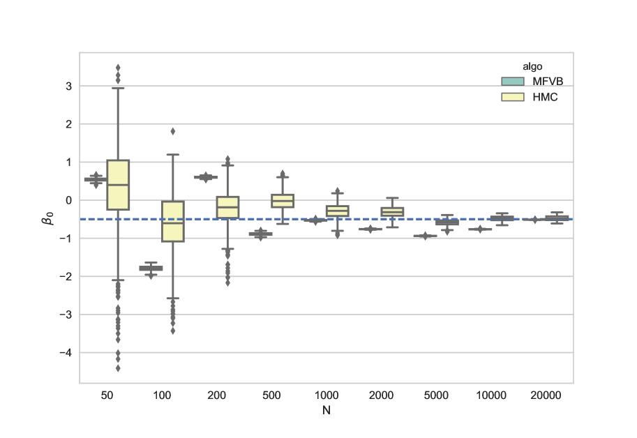
(a) Posterior of $\beta_{0}$

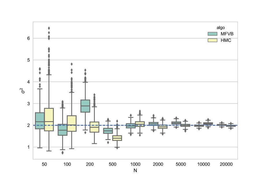
(b) Posterior of $\sigma^{2}$

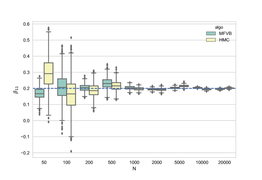
(c) Posterior of $\beta_{11}$

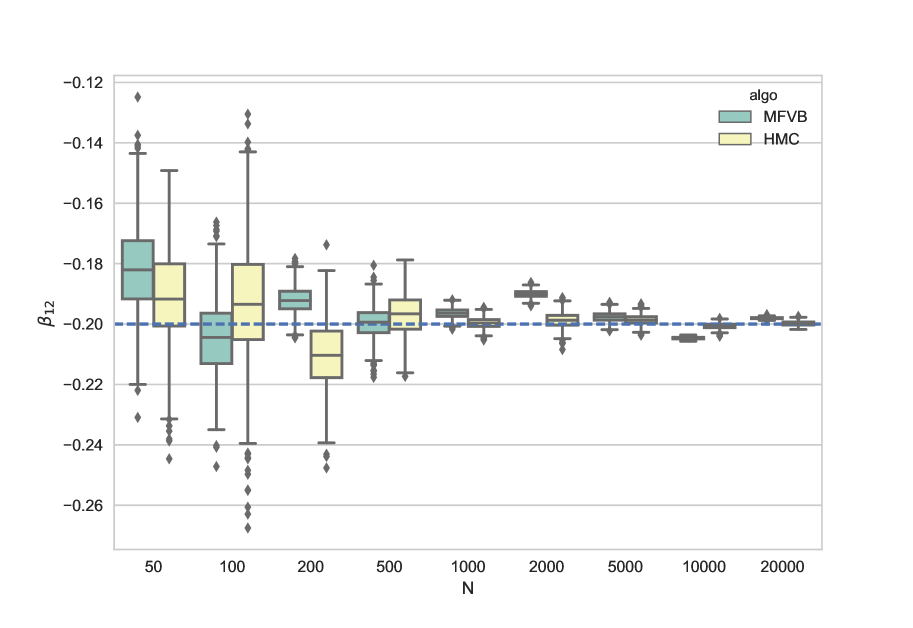
(d) Posterior of $\beta_{12}$

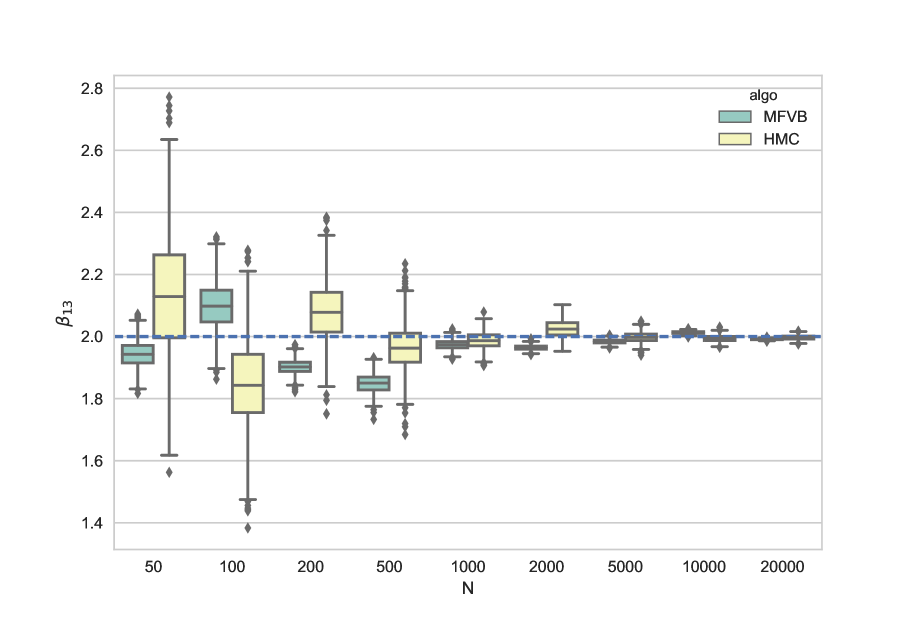
(e) Posterior of $\beta_{13}$

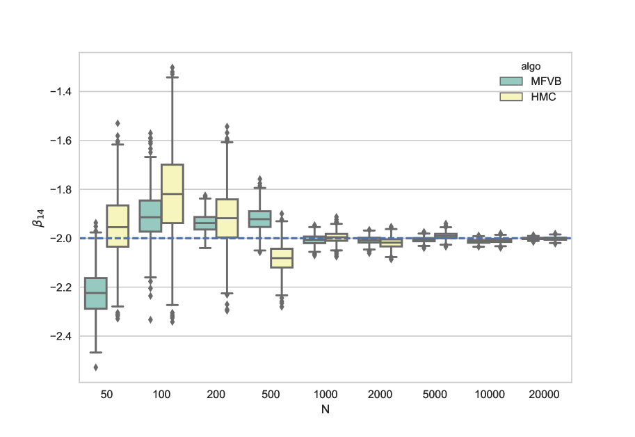
(f) Posterior of $\beta_{14}$

Figure 1: vb posteriors and hmc posteriors of Poisson Generalized Linear Mixed Model versus size of datasets. vb posteriors are consistent and asymptotically normal but underdispersed than hmc posteriors. $\beta_{0}$ and $\sigma^{2}$ converge to the truth slower than $\beta_{1}$ does. They echo our conclusions in Theorem 5 and Corollary 12.

5.2 Latent Dirichlet Allocation

Latent Dirichlet Allocation (lda) is a generative statistical model commonly adopted to describe word distributions in documents by latent topics.

Given $M$ documents, each with $N_{m},m=1,...,M$ words, composing a vocabulary of $V$ words, we assume $K$ latent topics. Consider two sets of latent variables: topic distributions for document $m$, $(\theta_{m})_{K\times 1}$, $m=1,...,M$ and word distributions for topic $k$, $(\phi_{k})_{V\times 1}$, $k=1,...,K$. The generative process is

$$\theta_{m}\sim p_{\theta}, m=1,...,M,$$

$$\phi_{k}\sim p_{\phi}, k=1,...,K,$$

$$z_{m,j}\sim \textrm{Mult}(\theta_{m}), j=1,...,N_{m},m=1,...,M,$$

$$w_{m,j}\sim \textrm{Mult}(\phi_{z_{m,j}}), j=1,...,N_{m},m=1,...,M.$$

The first two rows are assigning priors assigned to the latent variables. $w_{m,j}$ denotes word $j$ of document $m$ and $z_{m,j}$ denotes its assigned topic.

We simulate a data set with $V=100$ sized vocabulary and $K=10$ latent topics in $M=$ (10, 20, 50, 100, 200, 500, 100) documents. Each document has $N_{m}$ words where $N_{m}\stackrel{{\scriptstyle iid}}{{\sim}}$Poi(100). As the number of documents $M$ grows, the number of document-specific topic vectors $\theta_{m}$ grows while the number of topic-specific word vectors $\phi_{k}$ stays the same. In this sense, we consider $\theta_{m},m=1,...,M$ as local latent variables and $\phi_{k},k=1,...,K$ as global latent variables. We are interested in the vb posteriors of global latent variables $\phi_{k},k=1,...,K$ here. We generate the data sets with true values of $\theta$ and $\phi$, where they are random draws from $\theta_{m}\stackrel{{\scriptstyle iid}}{{\sim}}$Dir$((1/K)_{K\times 1})$ and $\phi_{k}\stackrel{{\scriptstyle iid}}{{\sim}}$Dir$((1/V)_{V\times 1})$.

Figure 2 presents the Kullback-Leibler (kl) divergence between the $K=10$ topic-specific word distributions induced by the true $\phi_{k}$’s and the fitted $\phi_{k}$’s by vb and hmc. This kl divergence equals to kl (Mult($\phi_{k}^{0}$)||Mult($\hat{\phi}_{k}))=\sum^{V}_{i=1}\phi_{ki}^{0}(\log\phi_{ki}^{0}-\log\hat{\phi}_{ki})$, where $\phi_{ki}^{0}$ is the $i$th entry of the true $k$th topic and $\hat{\phi}_{ki}$ is the $i$th entry of the fitted $k$th topic.

Figure 2a shows that vb posterior (dark blue) mean kl divergences of all $K=10$ topics get closer to 0 as the number of documents $M$ increase, faster than hmc (light blue). We become very close to the truth as the number of documents $M$ hits 1000. Figure 2b shows that the boxplots of vb posterior mean kl divergences get closer to 0 as $M$ increases. They are underdispersed compared to hmc posteriors. These align with our understanding of how vb posterior behaves in Theorem 5.

Computation wise, again vb is orders of magnitude faster than hmc. In particular, optimization in vb in our simulation studies converges within 10,000 steps.

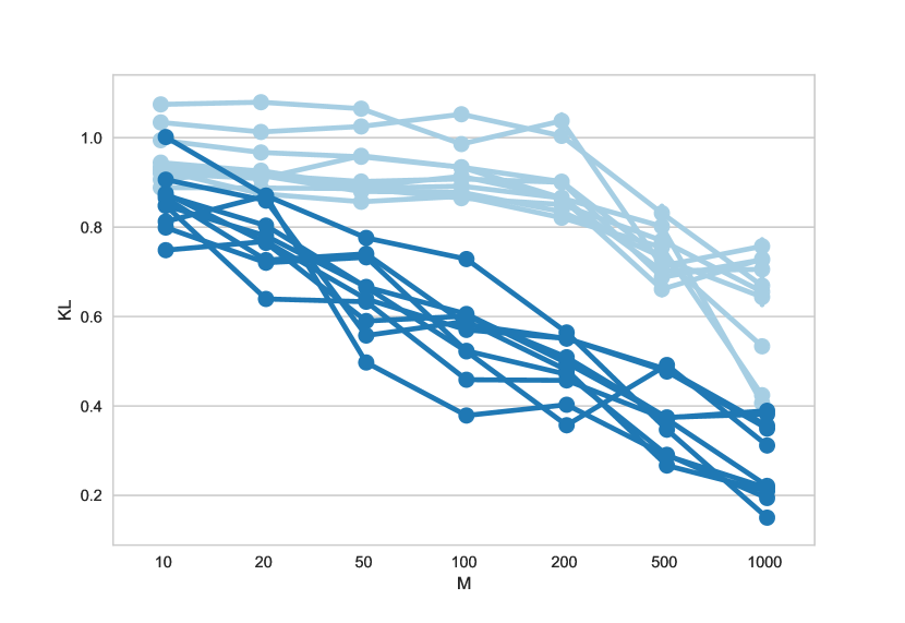
(a) Posterior mean kl divergence of the
$K=10$ topics

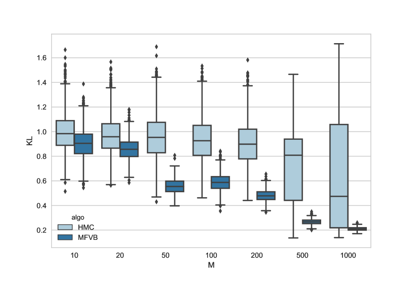
(b) Boxplots of posterior kl divergence of Topic 2

Figure 2: Mean of kl divergence between the true topics and the fitted vb and hmc posterior topics versus size of datasets. (a) vb posteriors (dark blue) converge to the truth; they are very close to the truth as we hit $M=1000$ documents. (b) vb posteriors are consistent but underdispersed compared to hmc posteriors (light blue). These align with our conclusions in Theorem 5.

6 Discussion

Variational Bayes (vb) methods are a fast alternative to Markov chain Monte Carlo (mcmc) for posterior inference in Bayesian modeling. However, few theoretical guarantees have been established. This work proves consistency and asymptotic normality for variational Bayes (vb) posteriors. The convergence is in the sense of total variation (tv) distance converging to zero in probability. In addition, we establish consistency and asymptotic normality of variational Bayes estimate (vbe). The result is frequentist in the sense that we assume a data generating distribution driven by some fixed nonrandom true value for global latent variables.

These results rest on ideal variational Bayes and its connection to frequentist variational approximations. Thus this work bridges the gap in asymptotic theory between the frequentist variational approximation, in particular the variational frequentist estimate (vfe), and variational Bayes. It also assures us that variational Bayes as a popular approximate inference algorithm bears some theoretical soundness.

We present our results in the classical vb framework but the results and proof techniques are more generally applicable. Our results can be easily generalized to more recent developments of vb beyond Kullback-Leibler (kl) divergence, $\alpha$-divergence or $\chi$-divergence for example (li2016renyi; dieng2017variational). They are also applicable to more expressive variational families, as long as they contain the mean field family. We could also allow for model misspecification, as long as the variational loglikelihood $M_{n}(\theta\,;\,x)$ under the misspecified model still enjoys local asymptotic normality.

There are several interesting avenues for future work. The variational Bernstein–von Mises theorem developed in this work applies to parametric and semiparametric models. One direction is to study the vb posteriors in nonparametric settings. A second direction is to characterize the finite-sample properties of vb posteriors. Finally, we characterized the asymptotics of an optimization problem, assuming that we obtain the global optimum. Though our simulations corroborated the theory, vb optimization typically finds a local optimum. Theoretically characterizing these local optima requires further study of the optimization loss surface.

Acknowledgements.   We thank the associate editor and two anonymous reviewers for their constructive comments. We thank Adji Dieng, Prateek Jaiswal, Christian Naesseth, and Dustin Tran for their valuable feedback on our manuscript. We also thank Richard Nickl for pointing us to a key reference. This work is supported by ONR N00014-11-1-0651, DARPA PPAML FA8750-14-2-0009, the Alfred P. Sloan Foundation, and the John Simon Guggenheim Foundation.

Appendix

Appendix A Proof of Lemma 1

What we need to show here is that our consistent testability assumption implies assumption (2.3) in kleijn2012bernstein:

$$\int_{\tilde{\theta}>M_{n}}\pi^{*}_{\tilde{\theta}}(\tilde{\theta}\leavevmode\nobreak\ |\leavevmode\nobreak\ x)\mathop{}\!\mathrm{d}\tilde{\theta}\stackrel{{\scriptstyle P_{\theta_{0}}}}{{\rightarrow}}0$$

for every sequence of constants $M_{n}\rightarrow\infty$, where $\tilde{\theta}=\delta_{n}^{-1}(\theta-\theta_{0}).$

This is a consequence of a slight generalization of Theorem 3.1 of kleijn2012bernstein. That theorem shows this implication for the iid case with a common $\sqrt{n}$-convergence rate for all dimensions of $\theta$. Specifically, they rely on a suitable test sequence under misspecification of uniform exponential power around the true value $\theta_{0}$ to split the posterior measure.

To show this implication in our case, we replace all $\sqrt{n}$ by $\delta_{n}^{-1}$ in the proofs of Theorem 3.1, Theorem 3.3, Lemma 3.3, Lemma 3.4 of kleijn2012bernstein. We refer the readers to kleijn2012bernstein and omit the proof here.

Appendix B Proof of Lemma 2

We first perform a change of variable step regarding the mean field variational family. In light of Lemma 1, we know that the vb ideal degenerates to a point mass at the rate of $\delta_{n}^{-1}$. We need to assume a variational family that degenerates to points masses at the same rate as the ideal vb posterior. This is because if the variational distribution converges to a point mass faster than $\pi(\theta\leavevmode\nobreak\ |\leavevmode\nobreak\ x)$, then the kl divergence between them will converge to $+\infty$. This makes the kl minimization meaningless as $n$ increases.

To avoid this pathology, we assume a variational family for the rescaled and re-centered $\theta$, $\check{\theta}:=\delta_{n}^{-1}(\theta-\mu)$, for some $\mu\in\Theta$. This is a centered and scaled transformation of $\theta$, centered to an arbitrary $\mu$. (In contrast, the previous transformation $\tilde{\theta}$ was centering $\theta$ at the true $\theta_{0}$.) With this transformation, the variational family is

$$q_{\check{\theta}}(\check{\theta})=q(\mu+\delta_{n}\check{\theta})|\textrm{det}(\delta_{n})|,$$ (20)

where $q(\cdot)$ is the original mean field variational family. We will overload the notation in Section 1 and write this transformed family as $q(\theta)$ and the corresponding family $\mathcal{Q}^{d}$.

In this family, for each fixed $\mu$, $\theta$ degenerates to a point mass at $\mu$ as $n$ goes to infinity. $\mu$ is not necessarily equal to the true value $\theta_{0}$. We allow $\mu$ to vary throughout the parameter space $\Theta$ so that $\mathcal{Q}^{d}$ does not restrict what the distributions degenerate to. $\mathcal{Q}^{d}$ only constrains that the variational distribution degenerates to some point mass at the rate of $\delta_{n}$. This step also does not restrict the applicability of the theoretical results. In practice, we always have finite samples with fixed $n$, so assuming a fixed variational family for $\check{\theta}$ as opposed to $\theta$ amounts to a change of variable $\theta=\mu+\delta_{n}\check{\theta}$.

Next we show consistency of the kl minimizer of the vb ideal.

To show consistency, we need to show that the mass of the kl minimizer

$$q^{\ddagger}:=\operatorname*{arg\,min}_{q(\theta)\in\mathcal{Q}^{d}}\lx@glossaries@gls@link{acronym}{KL}{\leavevmode\textsc{kl}}(q(\theta)||\pi^{*}(\theta\leavevmode\nobreak\ |\leavevmode\nobreak\ x))$$

concentrates near $\theta_{0}$ as $n\rightarrow\infty$. That is,

$$\int_{B(\theta_{0},\xi_{n})}q^{\ddagger}(\theta)\mathop{}\!\mathrm{d}\theta\stackrel{{\scriptstyle P_{\theta_{0}}}}{{\rightarrow}}1,$$ (21)

for some $\xi_{n}\rightarrow 0$ as $n\rightarrow\infty$. This implies

$$q^{\ddagger}(\theta)\stackrel{{\scriptstyle d}}{{\rightarrow}}\delta_{\theta_{0}}$$

in $P_{\theta_{0}}$-probability.

To begin with, we first claim that

$$\limsup_{n\rightarrow\infty}\min\lx@glossaries@gls@link{acronym}{KL}{\leavevmode\textsc{kl}}(q(\theta)||\pi^{*}(\theta\leavevmode\nobreak\ |\leavevmode\nobreak\ x))\leq M,$$ (22)

for some constant $M>0$, and

$$\int_{\mathbb{R}^{d}\backslash K}q^{\ddagger}(\theta)\mathop{}\!\mathrm{d}\theta\stackrel{{\scriptstyle}}{{\rightarrow}}0,$$ (23)

where $K$ is the compact set assumed in the local asymptotic normality condition.

The first claim says that the limiting minimum kl divergence is upper bounded. The intuition is that a choice of $q(\theta)$ with $\mu=\theta_{0}$ would have a finite kl divergence in the limit. This is because (rougly) $\pi^{*}(\theta\leavevmode\nobreak\ |\leavevmode\nobreak\ x)$ converges to a normal distribution centered at $\theta_{0}$ with rate $\delta_{n}$, so it suffices to have a $q(\theta)$ that shares the same center and the same rate of convergence.

The second claim says that the restriction of $q^{\ddagger}(\theta)$ to the compact set $K$, due to the set compactness needed in the local asymptotic normality (lan) condition, will not affect our conclusion in the limit. This is because the family of $\mathcal{Q}^{d}$ we assume has a shrinking-to-zero scale. In this way, as long as $\mu$ resides within $K$, $q^{\ddagger}(\theta)$ will eventually be very close to its renormalized restriction to the compact set $K$, $q^{\ddagger,K}(\theta)$, where

$$q^{\ddagger,K}(\theta)=\frac{q^{\ddagger}(\theta)\cdot\mathbb{I}_{\theta}(K)}{\int q^{\ddagger}(\theta)\cdot\mathbb{I}_{\theta}(K)\mathop{}\!\mathrm{d}\theta}.$$

We will prove these claims at the end.

To show $\int_{B(\theta_{0},\xi_{n})}q^{\ddagger,K}(\theta)\mathop{}\!\mathrm{d}\theta\stackrel{{\scriptstyle P_{\theta_{0}}}}{{\rightarrow}}1,$ we both upper bound and lower bound this integral. This step mimicks the Step 2 in the proof of Lemma 3.6 along with Lemma 3.7 in lu2016gaussapprox.

We first upper bound the integral using the lan condition,

$$\int q^{\ddagger,K}(\theta)M_{n}(\theta\,;\,x)\mathop{}\!\mathrm{d}\theta$$ (24)

$$= \int q^{\ddagger,K}(\theta)$$

$$\times\left[M_{n}(\theta_{0}\,;\,x)+\delta_{n}^{-1}(\theta-\theta_{0})^{\top}V_{\theta_{0}}\Delta_{n,\theta_{0}}-\frac{1}{2}[\delta_{n}^{-1}(\theta-\theta_{0})]^{\top}V_{\theta_{0}}[\delta_{n}^{-1}(\theta-\theta_{0})]+o_{P}(1)\right]\mathop{}\!\mathrm{d}\theta$$ (25)

$$\leq M_{n}(\theta_{0}\,;\,x)-C_{1}\sum_{i=1}^{d}\frac{\eta^{2}}{\delta_{n,ii}^{2}}\int_{B(\theta_{0},\eta)^{c}}q^{\ddagger,K}(\theta)\mathop{}\!\mathrm{d}\theta+o_{P}(1),$$ (26)

for large enough $n$ and $\eta<<1$ and some constant $C_{1}>0$. The first equality is due to the lan condition. The second inequality is due to the domination of quadratic term for large $n$.

Then we lower bound the integral using our first claim. By

$$\limsup_{n\rightarrow\infty}\lx@glossaries@gls@link{acronym}{KL}{\leavevmode\textsc{kl}}(q^{\ddagger,K}(\theta)||\pi^{*}(\theta\leavevmode\nobreak\ |\leavevmode\nobreak\ x))\leq M,$$

we can have

$$\int q^{\ddagger,K}(\theta)M_{n}(\theta\,;\,x)\mathop{}\!\mathrm{d}\theta\geq M_{n}(\theta_{0}\,;\,x)-M_{0},$$ (27)

for some large constant $M_{0}>M$.

This step is due to a couple of steps of technical calculation and the lan condition. To show this implication, we first rewrite the kl divergence as follows.

$$\lx@glossaries@gls@link{acronym}{KL}{\leavevmode\textsc{kl}}(q^{\ddagger,K}(\theta)||\pi^{*}(\theta\leavevmode\nobreak\ |\leavevmode\nobreak\ x))$$ (28)

$$= \int q^{\ddagger,K}(\theta)\log q^{\ddagger,K}(\theta)\mathop{}\!\mathrm{d}\theta-\int q^{\ddagger,K}(\theta)\log\pi^{*}(\theta\leavevmode\nobreak\ |\leavevmode\nobreak\ x)\mathop{}\!\mathrm{d}\theta$$ (29)

$$= \sum_{i=1}^{d}\int[\delta_{n,ii}^{-1}q_{h,i}^{\ddagger,K}(h)]\log[\delta_{n,ii}^{-1}q_{h,i}^{\ddagger,K}(h)]\delta_{n,ii}\mathop{}\!\mathrm{d}h-\int q^{\ddagger,K}(\theta)\log\pi^{*}(\theta\leavevmode\nobreak\ |\leavevmode\nobreak\ x)\mathop{}\!\mathrm{d}\theta$$ (30)

$$= \log|\det(\delta_{n})|^{-1}+\sum^{d}_{i=1}\mathbb{H}(q_{h,i}^{\ddagger,K}(h))-\int q^{\ddagger,K}(\theta)\log\pi^{*}(\theta\leavevmode\nobreak\ |\leavevmode\nobreak\ x)\mathop{}\!\mathrm{d}\theta,$$ (31)

where this calculation is due to the form of the $\mathcal{Q}^{d}$ family we assume and a change of variable of $h=\delta_{n}^{-1}(\theta-\mu)$; $h$ is in the same spirit as $\check{\theta}$ above. Notation wise, $\mu$ is the location parameter specific to $q^{\ddagger,K}(\theta)$ and $\mathbb{H}(q_{h}(h))$ denotes the entropy of distribution $q_{h}$.

We further approximate the last term by the lan condition.

$$\int q^{\ddagger,K}(\theta)\log\pi^{*}(\theta\leavevmode\nobreak\ |\leavevmode\nobreak\ x)\mathop{}\!\mathrm{d}\theta$$ (32)

$$= \int q^{\ddagger,K}(\theta)\log\frac{p(\theta)\exp(M_{n}(\theta\,;\,x))}{\int p(\theta)\exp(M_{n}(\theta\,;\,x))\mathop{}\!\mathrm{d}\theta}\mathop{}\!\mathrm{d}\theta$$ (33)

$$= \int q^{\ddagger,K}(\theta)\log p(\theta)\mathop{}\!\mathrm{d}\theta+\int q(\theta)M_{n}(\theta\,;\,x)\mathop{}\!\mathrm{d}\theta-\log\int p(\theta)\exp(M_{n}(\theta\,;\,x))\mathop{}\!\mathrm{d}\theta$$ (34)

$$= \int q^{\ddagger,K}(\theta)\log p(\theta)\mathop{}\!\mathrm{d}\theta+\int q^{\ddagger,K}(\theta)M_{n}(\theta\,;\,x)\mathop{}\!\mathrm{d}\theta$$

$$-\left[\frac{d}{2}\log(2\pi)-\frac{1}{2}\log\det V_{\theta_{0}}+\log\det(\delta_{n})+M_{n}(\theta_{0}\,;\,x)+\log p(\theta_{0})+o_{P}(1)\right].$$ (35)

This first equality is due to the definition of $\pi^{*}(\theta\leavevmode\nobreak\ |\leavevmode\nobreak\ x)$. The second equality is due to $\int q^{\ddagger,K}(\theta)\mathop{}\!\mathrm{d}\theta=1$. The third equality is due to Laplace approximation and the lan condition.

Going back to the kl divergence, this approximation gives

$$\lx@glossaries@gls@link{acronym}{KL}{\leavevmode\textsc{kl}}(q^{\ddagger,K}(\theta)||\pi^{*}(\theta\leavevmode\nobreak\ |\leavevmode\nobreak\ x))$$ (36)

$$= \log|\det(\delta_{n})|^{-1}+\sum^{d}_{i=1}\mathbb{H}(q_{h,i}^{\ddagger,K}(h))-\int q^{\ddagger,K}(\theta)\log\pi^{*}(\theta\leavevmode\nobreak\ |\leavevmode\nobreak\ x)\mathop{}\!\mathrm{d}\theta$$ (37)

$$= \log|\det(\delta_{n})|^{-1}+\sum^{d}_{i=1}\mathbb{H}(q_{h,i}^{\ddagger,K}(h))-\int q^{\ddagger,K}(\theta)\log p(\theta)\mathop{}\!\mathrm{d}\theta-\int q^{\ddagger,K}(\theta)M_{n}(\theta\,;\,x)\mathop{}\!\mathrm{d}\theta$$

$$+\left[\frac{d}{2}\log(2\pi)-\frac{1}{2}\log\det V_{\theta_{0}}+\log\det(\delta_{n})+M_{n}(\theta_{0}\,;\,x)+\log p(\theta_{0})+o_{P}(1)\right]$$ (38)

$$= \sum^{d}_{i=1}\mathbb{H}(q_{h,i}^{\ddagger,K}(h))-\int q^{\ddagger,K}(\theta)\log p(\theta)\mathop{}\!\mathrm{d}\theta-\int q^{\ddagger,K}(\theta)M_{n}(\theta\,;\,x)\mathop{}\!\mathrm{d}\theta$$

$$+\frac{d}{2}\log(2\pi)-\frac{1}{2}\log\det V_{\theta_{0}}+M_{n}(\theta_{0}\,;\,x)+\log p(\theta_{0})+o_{P}(1).$$ (39)

The first equality is exactly Equation 31. The second equality is due to Equation 35. The third equality is due to the cancellation of the two $\log\det(\delta_{n})$ terms. This exemplifies why we assumed the convergence rate of the $\mathcal{Q}^{d}$ family in the first place; we need to avoid the kl divergence going to infinity.

By

$$\limsup_{n\rightarrow\infty}\lx@glossaries@gls@link{acronym}{KL}{\leavevmode\textsc{kl}}(q^{\ddagger,K}(\theta)||\pi^{*}(\theta\leavevmode\nobreak\ |\leavevmode\nobreak\ x))\leq M,$$

we have

$$\int q^{\ddagger,K}(\theta)M_{n}(\theta\,;\,x)\mathop{}\!\mathrm{d}\theta$$ (40)

$$\geq -M+\sum^{d}_{i=1}\mathbb{H}(q_{h,i}^{\ddagger,K}(h))-\int q^{\ddagger,K}(\theta)\log p(\theta)\mathop{}\!\mathrm{d}\theta$$

$$+\frac{d}{2}\log(2\pi)-\frac{1}{2}\log\det V_{\theta_{0}}+M_{n}(\theta_{0}\,;\,x)+\log p(\theta_{0})+o_{P}(1)$$ (41)

$$\geq -M_{0}+M_{n}(\theta_{0}\,;\,x)+o_{P}(1)$$ (42)

for some constant $M_{0}>0$. This can be achieved by choosing a large enough $M_{0}$ to make the last inequality true. This is doable because all the terms does not change with $n$ except $\int q^{\ddagger,K}(\theta)\log p(\theta)\mathop{}\!\mathrm{d}\theta$. And we have $\limsup_{n\rightarrow\infty}\int q^{\ddagger,K}(\theta)\log p(\theta)\mathop{}\!\mathrm{d}\theta<\infty$ due to our prior mass condition.

Now combining Equation 42 and Equation 26, we have

$$M_{n}(\theta_{0}\,;\,x)-C_{1}\sum_{i=1}^{d}\frac{\eta^{2}}{\delta_{n,ii}^{2}}\int_{B(\theta_{0},\eta)^{c}}q^{\ddagger,K}(\theta)\mathop{}\!\mathrm{d}\theta+o_{P}(1)\geq -M_{0}+M_{n}(\theta_{0}\,;\,x).$$

This gives

$$\int_{B(\theta_{0},\eta)^{c}}q^{\ddagger,K}(\theta)\mathop{}\!\mathrm{d}\theta+o_{P}(1)\leq\frac{M_{0}\cdot(\min_{i}\delta_{n,ii})^{2}}{C_{2}\eta^{2}},$$

for some constant $C_{2}>0$. The right side of the inequality will go to zero as $n$ goes to infinity if we choose $\eta=\sqrt{M_{0}(\min_{i}\delta_{n,ii})/C_{2}}\rightarrow 0$. That is, we just showed Equation 21 with $\xi_{n}=\eta$.

We are now left to show the two claims we made at the beginning.

To show Equation 22, it suffices to show that there exists a choice of $q(\theta)$ such that

$$\limsup_{n\rightarrow\infty}\lx@glossaries@gls@link{acronym}{KL}{\leavevmode\textsc{kl}}(q(\theta)||\pi^{*}(\theta\leavevmode\nobreak\ |\leavevmode\nobreak\ x))<\infty.$$

We choose $\tilde{q}(\theta)=\prod_{i=1}^{d}N(\theta_{i};\theta_{0,i},\delta^{2}_{n,ii}v_{i})$ for $v_{i}>0,i=1,...,d$. We thus have

$$\lx@glossaries@gls@link{acronym}{KL}{\leavevmode\textsc{kl}}(\tilde{q}(\theta)||\pi^{*}(\theta\leavevmode\nobreak\ |\leavevmode\nobreak\ x))$$ (43)

$$= \sum^{d}_{i=1}\frac{1}{2}\log(v_{i})+\frac{d}{2}+d\log(2\pi)-\int\tilde{q}(\theta)\log p(\theta)\mathop{}\!\mathrm{d}\theta-\int\tilde{q}(\theta)M_{n}(\theta\,;\,x)\mathop{}\!\mathrm{d}\theta$$

$$-\frac{1}{2}\log\det V_{\theta_{0}}+M_{n}(\theta_{0}\,;\,x)+\log p(\theta_{0})+o_{P}(1)$$ (44)

$$= \sum^{d}_{i=1}\frac{1}{2}\log(v_{i})+\frac{d}{2}+d\log(2\pi)-\log p(\theta_{0})-M_{n}(\theta_{0}\,;\,x)$$

$$-\frac{1}{2}\log\det V_{\theta_{0}}+M_{n}(\theta_{0}\,;\,x)+\log p(\theta_{0})+o_{P}(1)$$ (45)

$$= \sum^{d}_{i=1}\frac{1}{2}\log(v_{i})+\frac{d}{2}+d\log(2\pi)-\frac{1}{2}\log\det V_{\theta_{0}}+C_{6}+o_{P}(1),$$ (46)

for some constant $C_{6}>0.$ The finiteness of limsup is due to the last term being bounded in the limit. The first equality is due to the same calculation as in Equation 45. The third equality is due to the cancellation of the two $M_{n}(\theta_{0}\,;\,x)$ terms and the two $p(\theta_{0})$ terms; this renders the whole term independent of $n$. The second equality is due to the limit of $\tilde{q}(\theta)$ concentrating around $\theta_{0}$. Specifically, we expand $\log p(\theta)$ to the second order around $\theta_{0}$,

$$\int\tilde{q}(\theta)\log p(\theta)\mathop{}\!\mathrm{d}\theta$$ (47)

$$= \log p(\theta_{0})+\int\tilde{q}(\theta)\left[(\theta-\theta_{0})(\log p(\theta_{0}))^{\prime}+\frac{(\theta-\theta_{0})^{2}}{2}\int_{0}^{1}(\log p(\xi\theta+(1-\xi)\theta_{0}))^{\prime\prime}(1-\xi)^{2}\mathop{}\!\mathrm{d}\xi\right]\mathop{}\!\mathrm{d}\theta$$ (48)

$$\leq \log p(\theta_{0})+\frac{1}{2!}\max_{\xi\in[0,1]}\left\{\int\tilde{q}(\theta)(\theta-\theta_{0})^{2}(\log p(\xi\theta+(1-\xi)\theta_{0}))^{\prime\prime}\mathop{}\!\mathrm{d}\theta\right\}$$ (49)

$$\leq \log p(\theta_{0})+\frac{M_{p}}{\sqrt{(2\pi)^{d}\det(\delta_{n}^{2})\prod_{i}v_{i}}}\int_{\mathbb{R}^{d}}|\theta|^{2}e^{(|\theta|+|\theta_{0}|)^{2}}\cdot e^{-\frac{1}{2}\theta^{\top}(\delta_{n}V\delta_{n})^{-1}\theta}\mathop{}\!\mathrm{d}\theta$$ (50)

$$\leq \log p(\theta_{0})+\frac{M_{p}}{\sqrt{(2\pi)^{d}\det(\delta_{n}^{2})\prod_{i}v_{i}}}e^{\theta_{0}^{2}}\int_{\mathbb{R}^{d}}|\theta|^{2}e^{-\frac{1}{2}\theta^{\top}[(\delta_{n}V\delta_{n})^{-1}-2I_{d}]\theta}$$ (51)

$$\leq \log p(\theta_{0})+C_{3}M_{p}e^{\theta_{0}^{2}}\max_{d}(\delta_{n,ii}^{2})\det(V^{-1}-2\delta_{n}^{2})^{-1}$$ (52)

$$\leq \log p(\theta_{0})+C_{4}\max_{d}(\delta_{n,ii}^{2})$$ (53)

where $\max_{d}(\delta_{n,ii}^{2})\rightarrow 0$ and $C_{3},C_{4}>0$. The first equality is due to Taylor expansion with integral form residuals. The second inequality is due to the first order derivative terms equal to zero and taking the maximum of the second order derivative. The third inequality is due to the prior mass condition where we assume the second derivative of $\log p(\theta)$ is bounded by $M_{p}e^{|\theta|^{2}}$ for some constant $M_{p}>0$. The fourth inequality is pulling $e^{\theta_{0}^{2}}$ out of the integral. The fifth inequality is due to rescaling $\theta$ by its covariance matrix and appealing to the mean of a Chi-squared distribution with $d$ degrees of freedom. The sixth (and last) inequality is due to $\det(V^{-1}-2\delta_{n}^{2})^{-1}>0$ for large enough $n$.

We apply the same Taylor expansion argument to the $\int\tilde{q}(\theta)M_{n}(\theta\,;\,x)\mathop{}\!\mathrm{d}\theta$.

$$\int_{K_{n}}\tilde{q}(\theta)M_{n}(\theta\,;\,x)\mathop{}\!\mathrm{d}\theta$$ (54)

$$= M_{n}(\theta_{0}\,;\,x)+\int_{K_{n}}\tilde{q}(\theta)\left[\delta_{n}^{-1}(\theta-\theta_{0})^{\top}V_{\theta_{0}}\Delta_{n,\theta_{0}}+\frac{1}{2}(\delta_{n}^{-1}(\theta-\theta_{0}))^{\top}V_{\theta_{0}}\delta_{n}^{-1}(\theta-\theta_{0})+o_{P}(1)\right]\mathop{}\!\mathrm{d}\theta$$ (55)

$$\leq M_{n}(\theta_{0}\,;\,x)+\frac{1}{2}Tr(V_{\theta_{0}}V)+o_{P}(1)$$ (56)

$$\leq M_{n}(\theta_{0}\,;\,x)+C_{6}+o_{P}(1)$$ (57)

where $K_{n}$ is a compact set. The first equality is due to the lan condition. The second inequality is due to $\tilde{q}(\theta)$ centered at $\theta_{0}$ with covariance $\delta_{n}V\delta_{n}$. The third inequalities are true for $C_{6}>0$.

For the set outside of this compact set $K_{n}$, we consider for a general choice of $q$ distribution, $\tilde{q}(\theta)=\mathcal{N}(\theta;\theta_{0}+\Delta_{n,\theta_{0}},\delta_{n}V_{\theta_{0}}\delta_{n}),$ of which $\tilde{q}(\theta)=\prod_{i=1}^{d}\mathcal{N}(\theta_{i};\theta_{0,i},\delta^{2}_{n,ii}v_{i})$ we work with is a special case.

$$\int_{\mathbb{R}^{d}\backslash K_{n}}\tilde{q}(\theta)(\log p(\theta)+M_{n}(\theta\,;\,x))\mathop{}\!\mathrm{d}\theta$$ (58)

$$\leq C_{7}\int_{\mathbb{R}^{d}\backslash K_{n}}\mathcal{N}(\theta;\theta_{0}+\Delta_{n,\theta_{0}},\delta_{n}V_{\theta_{0}}\delta_{n})(\log p(\theta)+M_{n}(\theta\,;\,x))\mathop{}\!\mathrm{d}\theta$$ (59)

$$\leq C_{8}[\det(\delta_{n})^{-1}\log(\det(\delta_{n})^{-1})]\int_{\mathbb{R}^{d}\backslash K_{n}}\mathcal{N}(\tilde{\theta};\Delta_{n,\theta_{0}},V_{\theta_{0}})\log\pi^{*}(\tilde{\theta}\leavevmode\nobreak\ |\leavevmode\nobreak\ x)\det(\delta_{n})\mathop{}\!\mathrm{d}\tilde{\theta}$$ (60)

$$\leq C_{9}\log(\det(\delta_{n})^{-1})]\int_{\mathbb{R}^{d}\backslash K_{n}}[\pi^{*}(\tilde{\theta}\leavevmode\nobreak\ |\leavevmode\nobreak\ x)+o_{P}(1)]\log\pi^{*}(\tilde{\theta}\leavevmode\nobreak\ |\leavevmode\nobreak\ x),V_{\theta_{0}})\mathop{}\!\mathrm{d}\tilde{\theta}$$ (61)

$$\leq C_{10}\log(\det(\delta_{n})^{-1})]\int_{\mathbb{R}^{d}\backslash K_{n}}[\mathcal{N}(\tilde{\theta};\Delta_{n,\theta_{0}},V_{\theta_{0}})+o_{P}(1)]\log\mathcal{N}(\tilde{\theta};\Delta_{n,\theta_{0}},V_{\theta_{0}})\mathop{}\!\mathrm{d}\tilde{\theta}$$ (62)

$$\leq o_{P}(1)$$ (63)

for some $C_{7},C_{8},C_{9},C_{10}>0$. The first inequality is due to $\tilde{q}(\theta)$ centered at $\theta_{0}$ and with rate of convergence $\delta_{n}$. The second inequality is due to a change of variable $\tilde{\theta}=\delta_{n}^{-1}(\theta-\theta_{0})$. The third inequality is due to Lemma 1. The fourth inequality is due to Lemma 1 and Theorem 2 in piera2009convergence. The fifth inequality is due to a choice of fast enough increasing sequence of compact sets $K_{n}$.

The lower bound of $\int\tilde{q}(\theta)(\log p(\theta)+M_{n}(\theta\,;\,x))\mathop{}\!\mathrm{d}\theta$ can be derived with exactly the same argument. Our first claim Equation 22 is thus proved.

To show our second claim Equation 23, we first denote $B(\mu,M)$ as the largest ball centered at $\mu$ and contained in the compact set $K$. We know by the construct of $\mathcal{Q}^{d}$ — $\mathcal{Q}^{d}$ has a shrinking-to-zero scale — that for each $\epsilon>0$, there exists an $N$ such that for all $n>N$ we have $\int_{{||\theta-\mu||>M}}q(\theta)\mathop{}\!\mathrm{d}\theta<\epsilon.$ Therefore, we have

$$\int_{\mathbb{R}^{d}\backslash K}q^{\ddagger}(\theta)\mathop{}\!\mathrm{d}\theta\leq\int_{\mathbb{R}^{d}\backslash B(\mu,M)}q^{\ddagger}(\theta)\mathop{}\!\mathrm{d}\theta\leq\epsilon.$$

Appendix C Proof of Lemma 3

To show the convergence of optimizers from two minimization problems, we invoke $\Gamma$-convergence. It is a classical technique in characterizing variational problems. A major reason is that if two functionals $\Gamma-$converge, then their minimizer also converge.

We recall the definition of $\Gamma$-convergence (dal2012introduction; braides2006handbook).

Definition 14.

Let $\mathcal{X}$ be a metric space and $F_{\epsilon}:\mathcal{X}\rightarrow\mathbb{R}$ a family of functionals indexed by $\epsilon>0.$ Then the existence of a limiting functional $F_{0}$, the $\Gamma-$limit of $F_{\epsilon}$, as $\epsilon\rightarrow 0$, relies on two conditions:

1. (liminf inequality) for every $x\in\mathcal{X}$ and for every $x_{\epsilon}\rightarrow x$, we have

   $$F_{0}(x)\leq\liminf_{\epsilon\rightarrow 0}F_{\epsilon}(x_{\epsilon}),$$

2. (limsup inequality / existence of a recovery sequence) for every $x\in\mathcal{X}$ we can find a sequence $\bar{x}_{\epsilon}\rightarrow x$ such that

   $$F_{0}(x)\geq\limsup_{\epsilon\rightarrow 0}F_{\epsilon}(\bar{x}_{\epsilon}).\\$$

The first condition says that $F_{0}$ is a lower bound for the sequence $F_{\epsilon}$, in the sense that $F_{0}(x)\leq F_{\epsilon}(x_{\epsilon})+o(1)$ whenever $x_{\epsilon}\rightarrow x$. Together with the first condition, the second condition implies that $F_{0}(x)=\lim_{\epsilon\rightarrow 0}F_{\epsilon}(\bar{x}_{\epsilon}),$ so that the lower bound is sharp.

$\Gamma$-convergence is particularly useful for variational problems due to the following fundamental theorem. Before stating the theorem, we first define equi-coerciveness.

Definition 15.

(Equi-coerciveness of functionals) A sequence $F_{\epsilon}:\mathcal{X}\rightarrow\bar{\mathbb{R}}$ is equi-coercise if for all $\epsilon_{j}\rightarrow 0$ and $x_{j}$ such that $F_{\epsilon_{j}}(x_{j})\leq t$ there exist a subsequence of $j$ (not relabeled) and a converging sequence $x^{\prime}_{j}$ such that $F_{\epsilon_{j}}(x^{\prime}_{j})\leq F_{\epsilon_{j}}(x_{j})+o(1)$.

Equi-coerciveness of functionals ensures that we can find a precompact minimizing sequence of $F_{\epsilon}$ such that the convergence $x_{\epsilon}\rightarrow x$ can take place. Now we are ready to state the fundamental theorem.

Theorem 16.

(Fundamental theorem of $\Gamma$-convergence) Let $\mathcal{X}$ be a metric space. Let $(F_{\epsilon})$ be an equi- coercise sequence of functions on $\mathcal{X}$. Let $F=\Gamma-\lim_{\epsilon\rightarrow 0}F_{\epsilon}$, then

$$\operatorname*{arg\,min}_{\mathcal{X}}F=\lim_{\epsilon\rightarrow 0}\operatorname*{arg\,min}_{\mathcal{X}}F_{\epsilon}.\\$$

The above theorem implies that if all functions $F_{\epsilon}$ admit a minimizer $x_{\epsilon}$ then, up to subsequences, $x_{\epsilon}$ converge to a minimum point of $F$. We remark that the converse is not true; we may have minimizers of $F$ which are not limits of minimizers of $F_{\epsilon}$, e.g. $F_{\epsilon}(t)=\epsilon t^{2}$ (braides2006handbook).

In this way, $\Gamma$-convergence is convenient to use when we would like to study the asymptotic behavior of a family of problem $F_{\epsilon}$ through defining a limiting problem $F_{0}$ which is a ‘good approximation’ such that the minimizers converge: $x_{\epsilon}\rightarrow x_{0}$, where $x_{0}$ is a minimizer of $F_{0}$. Conversely, we can characterize solutions of a difficult $F_{0}$ by finding easier approximating $F_{\epsilon}$ (braides2006handbook).

We now prove Lemma 3 for the general mean field family. The family is parametric as in Section 1, so we assume it is indexed by some finite dimensional parameter $m$. We want to show that the functionals

$$F_{n}(m):=\lx@glossaries@gls@link{acronym}{KL}{\leavevmode\textsc{kl}}(q(\theta;m)||\pi^{*}(\theta\leavevmode\nobreak\ |\leavevmode\nobreak\ x))$$

$\Gamma$-converge to

$$F_{0}(m):=\lx@glossaries@gls@link{acronym}{KL}{\leavevmode\textsc{kl}}(q(\theta;m)||\mathcal{N}(\theta;\theta_{0}+\delta_{n}\Delta_{n,\theta_{0}},\delta_{n}V_{\theta_{0}}^{-1}\delta_{n}))-\Delta_{n,\theta_{0}}^{\top}V_{\theta_{0}}\Delta_{n,\theta_{0}}$$

in probability as $n\rightarrow 0$. Recall that the mean field family has density

$$q(\theta)=\prod^{d}_{i=1}\delta_{n,ii}^{-1}q_{h,i}(h),$$

where $h=\delta_{n}^{-1}(\theta-\theta_{0}).$

We need the following mild technical conditions on $\mathcal{Q}^{d}$.

Following the change-of-variable step detailed in the beginning of Appendix B, we consider the mean field variational family with densities $q(\theta)=\prod^{d}_{i=1}\delta_{n,ii}^{-1}q_{h,i}(h),$ where $h=\delta_{n}^{-1}(\theta-\mu)$ for some $\mu\in\Theta$.

Assumption 2.

We assume the following conditions on $q_{h,i}$:

1. $q_{h,i},i=1,...,d$ have continuous densities.

2. $q_{h,i},i=1,...,d$ have positive and finite entropies.

3. $\int q_{h,i}^{\prime}(h)\mathop{}\!\mathrm{d}h<\infty,i=1,...,d.$
   

The last condition ensures that convergence in finite dimensional parameters imlied convergence in tv distance. This is due to a Taylor expansion argument:

$$\lx@glossaries@gls@link{acronym}{KL}{\leavevmode\textsc{kl}}(q(\theta;m)||q(\theta;m+\delta))$$ (64)

$$= \int q(\theta;m)\cdot(\log q(\theta;m)-\log q(\theta;m+\delta))\mathop{}\!\mathrm{d}\theta$$ (65)

$$= \int q(\theta;m)\cdot(\delta\cdot(\log q(\theta;m))^{\prime})\mathop{}\!\mathrm{d}\theta+o(1)$$ (66)

$$= \delta\int(q(\theta;m))^{\prime}\mathop{}\!\mathrm{d}\theta$$ (67)

$$< \epsilon$$ (68)

The last step is true if 2 is true for $q$. We also notice that convergence in kl divergence implies convergence in tv distance. Therefore, 2 implies that convergence in finite dimensional parameter implies convergence in tv distance.

Together with Theorem 16, the $\Gamma$-convergence of the two functionals implies $m_{n}\stackrel{{\scriptstyle P_{\theta_{0}}}}{{\rightarrow}}m_{0}$ where $m_{n}$ is the minimizer of $F_{n}$ for each $n$ and $m_{0}$ is the minimizer of $F_{0}$. This is due to the last term of $F_{0}$ – $\Delta_{n,\theta_{0}}^{\top}V_{\theta_{0}}\Delta_{n,\theta_{0}}$ is a constant bounded in $P_{\theta_{0}}$ probability and independent of $m$. The convergence in total variation then follows from 2 and our argument above.

Lastly, we prove the $\Gamma$-convergence of the two functionals for the mean field family.

We first rewrite $F_{n}(m,\mu)$.

$$F_{n}(m,\mu):=\lx@glossaries@gls@link{acronym}{KL}{\leavevmode\textsc{kl}}(q(\theta;m,\mu)||\pi^{*}(\theta\leavevmode\nobreak\ |\leavevmode\nobreak\ x))$$ (69)

$$= \log|\det(\delta_{n})|^{-1}+\sum^{d}_{i=1}\mathbb{H}(q_{h,i}(h;m))-\int q(\theta;m,\mu)\log\pi^{*}(\theta\leavevmode\nobreak\ |\leavevmode\nobreak\ x))\mathop{}\!\mathrm{d}\theta$$ (70)

$$= \log|\det(\delta_{n})|^{-1}+\sum^{d}_{i=1}\mathbb{H}(q_{h,i}(h;m))-\int q(\theta;m,\mu)\log p(\theta)\mathop{}\!\mathrm{d}\theta-\int q(\theta;m,\mu)M_{n}(\theta\,;\,x)\mathop{}\!\mathrm{d}\theta$$

$$+\log\int p(\theta)\exp(M_{n}(\theta\,;\,x))\mathop{}\!\mathrm{d}\theta$$ (71)

$$= \log|\det(\delta_{n})|^{-1}+\sum^{d}_{i=1}\mathbb{H}(q_{h,i}(h;m))-\int q(\theta;m,\mu)\log p(\theta)\mathop{}\!\mathrm{d}\theta-\int q(\theta;m,\mu)M_{n}(\theta\,;\,x)\mathop{}\!\mathrm{d}\theta$$

$$+\left[\frac{d}{2}\log(2\pi)-\frac{1}{2}\log\det V_{\theta_{0}}+\log\det(\delta_{n})+M_{n}(\theta_{0}\,;\,x)+\log p(\theta_{0})+o_{P}(1)\right]$$ (72)

$$= \sum^{d}_{i=1}\mathbb{H}(q_{h,i}(h;m))-\int q(\theta;m,\mu)\log p(\theta)\mathop{}\!\mathrm{d}\theta-\int q(\theta;m,\mu)M_{n}(\theta\,;\,x)\mathop{}\!\mathrm{d}\theta$$

$$+\left[\frac{d}{2}\log(2\pi)-\frac{1}{2}\log\det V_{\theta_{0}}+M_{n}(\theta_{0}\,;\,x)+\log p(\theta_{0})+o_{P}(1)\right]$$ (73)

$$= \sum^{d}_{i=1}\mathbb{H}(q_{h,i}(h;m))-\int q(\theta;m,\mu)M_{n}(\theta\,;\,x)\mathop{}\!\mathrm{d}\theta+\log p(\theta_{0})-\log p(\mu)$$

$$+\left[\frac{d}{2}\log(2\pi)-\frac{1}{2}\log\det V_{\theta_{0}}+M_{n}(\theta_{0}\,;\,x)+o_{P}(1)\right]$$ (74)

$$= \sum^{d}_{i=1}\mathbb{H}(q_{h,i}(h;m))-\int q(\theta;m,\mu)[M_{n}(\theta_{0}\,;\,x)+\delta_{n}^{-1}(\theta-\theta_{0})^{\top}V_{\theta_{0}}\Delta_{n,\theta_{0}}+\log p(\theta_{0})-\log p(\mu)$$

$$-\frac{1}{2}(\delta_{n}^{-1}(\theta-\theta_{0}))^{\top}V_{\theta_{0}}\delta_{n}^{-1}(\theta-\theta_{0})+o_{P}(1)]\mathop{}\!\mathrm{d}\theta-\left[\frac{d}{2}\log(2\pi)-\frac{1}{2}\log\det V_{\theta_{0}}+M_{n}(\theta_{0}\,;\,x)+o_{P}(1)\right]$$ (75)

$$= \sum^{d}_{i=1}\mathbb{H}(q_{h,i}(h;m))-\int\delta_{n}^{-1}(\theta-\theta_{0})^{\top}V_{\theta_{0}}\Delta_{n,\theta_{0}}\cdot q(\theta;m,\mu)\mathop{}\!\mathrm{d}\theta$$

$$+\int\frac{1}{2}(\delta_{n}^{-1}(\theta-\theta_{0}))^{\top}V_{\theta_{0}}\delta_{n}^{-1}(\theta-\theta_{0})\cdot q(\theta;m,\mu)\mathop{}\!\mathrm{d}\theta-\left[\frac{d}{2}\log(2\pi)-\frac{1}{2}\log\det V_{\theta_{0}}+o_{P}(1)\right]$$ (76)

The first equality is by the definition of kl divergence. The second equality is by the definition of the vb ideal. The third equality is due to the Laplace approximation of the normalizer like we did in Equation 35. The fourth equality is due to the cancellation of the two $\log\det(\delta_{n})$ terms. This again exemplifies why we assume a fixed variational family on the rescale variable $\check{\theta}$. The fifth equality is due to a similar argument as in Equation 45. The sixth equality is due to the lan condition of $M_{n}(\theta\,;\,x)$. The seventh equality is due to the computation of each term in the integral as an expectation under the distribution $q(\theta)$. To extend the restriction to some compact set $K$ to the whole space $\mathbb{R}^{d}$ in the sixth equality, we employ the same argument as in Equation 46.

We notice that when $\mu\neq\theta_{0}$, we will have $F_{n}(m)\rightarrow\infty$. On the other hand, we have $\limsup F_{n}<\infty$. This echoes our consistency result in Lemma 2.

Now we rewrite $F_{0}(m,\mu)$.

$$\lx@glossaries@gls@link{acronym}{KL}{\leavevmode\textsc{kl}}(q(\theta;m,\mu)||\mathcal{N}(\theta;\theta_{0}+\delta_{n}\Delta_{n,\theta_{0}},\delta_{n}V_{\theta_{0}}^{-1}\delta_{n}))$$ (77)

$$= \log|\det(\delta_{n})|^{-1}+\sum^{d}_{i=1}\mathbb{H}(q_{h,i}(h;m))+\int q(\theta;m,\mu)\log\mathcal{N}(\theta;\theta_{0}+\delta_{n}\Delta_{n,\theta_{0}},\delta_{n}V_{\theta_{0}}^{-1}\delta_{n})\mathop{}\!\mathrm{d}\theta$$ (78)

$$= \log|\det(\delta_{n})|^{-1}+\sum^{d}_{i=1}\mathbb{H}(q_{h,i}(h;m))+\frac{d}{2}\log(2\pi)-\frac{1}{2}\log\det V_{\theta_{0}}+\log\det(\delta_{n})$$

$$+\int q(\theta;m,\mu)\cdot(\theta-\theta_{0}-\delta_{n}\Delta_{n,\theta_{0}})^{\top}\delta_{n}^{-1}V_{\theta_{0}}\delta_{n}^{-1}(\theta-\theta_{0}-\delta_{n}\Delta_{n,\theta_{0}})\mathop{}\!\mathrm{d}\theta$$ (79)

$$= \sum^{d}_{i=1}\mathbb{H}(q_{h,i}(h;m))+\frac{d}{2}\log(2\pi)-\frac{1}{2}\log\det V_{\theta_{0}}+\Delta_{n,\theta_{0}}^{\top}V_{\theta_{0}}\Delta_{n,\theta_{0}}$$

$$-\int\delta_{n}^{-1}(\theta-\theta_{0})^{\top}V_{\theta_{0}}\Delta_{n,\theta_{0}}\cdot q(\theta;m,\mu)\mathop{}\!\mathrm{d}\theta+\int\frac{1}{2}(\delta_{n}^{-1}(\theta-\theta_{0}))^{\top}V_{\theta_{0}}\delta_{n}^{-1}(\theta-\theta_{0})\cdot q(\theta;m,\mu)\mathop{}\!\mathrm{d}\theta.$$ (80)

This gives

$$F_{0}(m,\mu)-\Delta_{n,\theta_{0}}^{\top}V_{\theta_{0}}\Delta_{n,\theta_{0}}$$ (81)

$$= \sum^{d}_{i=1}\mathbb{H}(q_{h,i}(h;m))-\frac{d}{2}\log(2\pi)+\frac{1}{2}\log\det V_{\theta_{0}}$$

$$-\int\delta_{n}^{-1}(\theta-\theta_{0})^{\top}V_{\theta_{0}}\Delta_{n,\theta_{0}}\cdot q(\theta;m,\mu)\mathop{}\!\mathrm{d}\theta$$

$$+\int\frac{1}{2}(\delta_{n}^{-1}(\theta-\theta_{0}))^{\top}V_{\theta_{0}}\delta_{n}^{-1}(\theta-\theta_{0})\cdot q(\theta;m,\mu)\mathop{}\!\mathrm{d}\theta$$ (82)

$$= +\infty\cdot(1-\mathbb{I}_{\mu}(\theta_{0}))+[\sum^{d}_{i=1}\mathbb{H}(q_{h,i}(h;m))-\frac{d}{2}\log(2\pi)+\frac{1}{2}\log\det V_{\theta_{0}}$$

$$-\int\delta_{n}^{-1}(\theta-\theta_{0})^{\top}V_{\theta_{0}}\Delta_{n,\theta_{0}}\cdot q(\theta;m,\mu)\mathop{}\!\mathrm{d}\theta$$

$$+\int\frac{1}{2}(\delta_{n}^{-1}(\theta-\theta_{0}))^{\top}V_{\theta_{0}}\delta_{n}^{-1}(\theta-\theta_{0})\cdot q(\theta;m,\mu)\mathop{}\!\mathrm{d}\theta]\cdot\mathbb{I}_{\mu}(\theta_{0}).$$ (83)

The last step is due to our definition of our variational family $q(\theta;m,\mu)=\prod^{d}_{i=1}\delta_{n,ii}^{-1}q_{h,i}(h;m),$ where $h=\delta_{n}^{-1}(\theta-\mu)$ for some $\mu\in\Theta$. The last step is true as long as the $q_{h,i}$ distributions are not point masses at zero. This is ensured by positive entropy in 2.

Comparing Equation 76 and Equation 83, we can prove the $\Gamma$ convergence. Let $m_{n}\rightarrow m$. When $\mu\neq\theta_{0}$, $\liminf_{n\rightarrow\infty}F_{n}(m_{n},\mu)=+\infty$. The limsup inequality is automatically satisfied. When $\mu=\theta_{0}$, we have $F_{n}(m,\mu)=F_{0}(m,\mu)-\Delta_{n,\theta_{0}}^{\top}V_{\theta_{0}}\Delta_{n,\theta_{0}}+o_{P}(1)$. This implies $F_{0}(m,\mu)\leq\lim_{n\rightarrow\infty}F_{n}(m_{n},\mu)$ in $P_{\theta_{0}}$ probability by the continuity of $F_{n}$ ensured by 2.

We then show the existence of a recovery sequence. When $\mu\neq\theta_{0}$, $F_{0}(m,\mu)=+\infty$. The limsup inequality is automatically satisfied. When $\mu=\theta_{0}$, we can simply choose $m_{n}=\theta_{0}$. The limsup inequality is again ensured by $F_{0}(m,\mu)\leq\lim_{n\rightarrow\infty}F_{n}(m_{n},\mu)$ in $P_{\theta_{0}}$ probability and the continuity of $F_{n}$. The $\Gamma$-convergence of the $F$ functionals is shown.

We notice that $\Delta_{n,\theta_{0}}^{\top}V_{\theta_{0}}\Delta_{n,\theta_{0}}$ does not depend on $m$ or $\mu$ so that $\operatorname*{arg\,min}F_{0}=$ $\operatorname*{arg\,min}F_{0}-\Delta_{n,\theta_{0}}^{\top}V_{\theta_{0}}\Delta_{n,\theta_{0}}$. The convergence of the kl minimizers is thus proved.

Appendix D Proof of Lemma 4

Notice that the mean field variational families $\mathcal{Q}^{d}=\{q:q(\theta)=\prod^{d}_{i=1}\delta_{n,ii}^{-1}q_{h,i}(h),$ where $h=\delta_{n}^{-1}(\theta-\mu)$ for some $\mu\in\Theta\}$, or the Gaussian family $\{q:q(\theta)=N(m,\delta_{n}\Sigma\delta_{n})\}$ can be written in the form of

$$q(\theta)=|\det\delta_{n}|^{-1}q_{h}(\delta_{n}^{-1}(\theta-\mu))$$

for some $\mu\in\mathbb{R}^{d}$, and $\int q_{h}(h)\mathop{}\!\mathrm{d}h=0.$ This form is due to a change-of-variable step we detailed in the beginning of Appendix B.

We first specify the mild technical conditions on $\mathcal{Q}^{d}$.

Assumption 3.

We assume the following conditions on $q_{h}$.

1. If $q_{h}$ is has zero mean, we assume $\int h^{2}\cdot q_{h}(h)\mathop{}\!\mathrm{d}h<\infty$ and $\sup_{z,x}|(\log p(z,x\leavevmode\nobreak\ |\leavevmode\nobreak\ \theta))^{\prime\prime}|\leq C_{11}\cdot q_{h}(\theta)^{-C_{12}}$ for some $C_{11},C_{12}>0;$ $|M_{n}(\theta\,;\,x)^{\prime\prime}|\leq C_{13}\cdot q_{h}(\theta)^{-C_{14}}$ for some $C_{13},C_{14}>0.$

2. If $q_{h}$ has nonzero mean, we assume $\int h\cdot q_{h}(h)\mathop{}\!\mathrm{d}h<\infty$ and $\sup_{z,x}|(\log p(z,x\leavevmode\nobreak\ |\leavevmode\nobreak\ \theta))^{\prime}|\leq C_{11}\cdot q_{h}(\theta)^{-C_{12}}$ for some $C_{11},C_{12}>0$; $|M_{n}(\theta\,;\,x)^{\prime}\leq C_{13}|\cdot q_{h}(\theta)^{-C_{14}}$ for some $C_{13},C_{14}>0.$
   

The assumption first assumes finite moments for $q_{h}$ so that we can properly apply a Taylor expansion argument. The second part of this assumption makes sure the derivative of $\log p(z,x\leavevmode\nobreak\ |\leavevmode\nobreak\ \theta)$ does not increase faster than the tail decrease of $q_{h}(\cdot)$. For example, if $q_{h}(\cdot)$ is normal, then the second part writes $\sup_{z,x}|(\log p(z,x\leavevmode\nobreak\ |\leavevmode\nobreak\ \theta))^{\prime\prime}|\leq C_{15}\exp(\theta^{2})$ for some $C_{15}>0$, and $|M_{n}(\theta\,;\,x)^{\prime\prime}|\leq C_{13}\exp(\theta^{2})$ for some $C_{13}>0$. The latter is satisfied by the lan condition. This is in general a rather weak condition. We usually would not expect the derivative of $\log p(z,x\leavevmode\nobreak\ |\leavevmode\nobreak\ \theta)$ and $M_{n}(\theta\,;\,x)$ to increase this fast as $\theta$ increases.

Now we are ready to prove the lemma.

We first approximate the profiled evidence lower bound (elbo), $\lx@glossaries@gls@link{acronym}{ELBO}{\leavevmode\textsc{elbo}}_{p}(q(\theta))$.

$$\lx@glossaries@gls@link{acronym}{ELBO}{\leavevmode\textsc{elbo}}_{p}(q(\theta))$$ (84)

$$:= \sup_{q(z)}\int q(\theta)\left(\log\left[p(\theta)\exp\left\{\int q(z)\log\frac{p(x,z|\theta)}{q(z)}\mathop{}\!\mathrm{d}z\right\}\right]-\log q(\theta)\right)\mathop{}\!\mathrm{d}\theta,$$ (85)

$$= \int q(\theta)\log p(\theta)\mathop{}\!\mathrm{d}\theta-\int q(\theta)\log q(\theta)\mathop{}\!\mathrm{d}\theta+\sup_{q(z)}\int q(\theta)\int q(z)\log\frac{p(x,z|\theta)}{q(z)}\mathop{}\!\mathrm{d}z\mathop{}\!\mathrm{d}\theta$$ (86)

$$= \int q(\theta)\log p(\theta)\mathop{}\!\mathrm{d}\theta-\int q(\theta)\log q(\theta)\mathop{}\!\mathrm{d}\theta$$

$$+\sup_{q(z)}\int q(\theta)[\int q(z)\log\frac{p(x,z|\mu)}{q(z)}\mathop{}\!\mathrm{d}z+(\theta-\mu)\left(\int q(z)\log\frac{p(x,z|\mu)}{q(z)}\mathop{}\!\mathrm{d}z\right)^{\prime}$$

$$= \int q(\theta)\log p(\theta)\mathop{}\!\mathrm{d}\theta-\int q(\theta)\log q(\theta)\mathop{}\!\mathrm{d}\theta+\sup_{q(z)}\int q(z)\log\frac{p(x,z|\mu)}{q(z)}\mathop{}\!\mathrm{d}z$$

$$+\int q(\theta)\frac{1}{2}|\theta-\mu|^{2}\left(\int q(z)\log\frac{p(x,z|\tilde{\theta}^{\dagger})}{q(z)}\mathop{}\!\mathrm{d}z\right)^{\prime\prime}]\mathop{}\!\mathrm{d}\theta$$ (87)

$$\geq \int q(\theta)\log p(\theta)\mathop{}\!\mathrm{d}\theta-\int q(\theta)\log q(\theta)\mathop{}\!\mathrm{d}\theta+\sup_{q(z)}\int q(z)\log\frac{p(x,z|\mu)}{q(z)}\mathop{}\!\mathrm{d}z$$

$$-C_{15}\int q(\theta)\frac{1}{2}|\theta-\mu|^{2}q_{h}(\theta)^{-C_{12}}\mathop{}\!\mathrm{d}\theta$$ (88)

$$= \int q(\theta)\log p(\theta)\mathop{}\!\mathrm{d}\theta-\int q(\theta)\log q(\theta)\mathop{}\!\mathrm{d}\theta+\sup_{q(z)}\int q(z)\log\frac{p(x,z|\mu)}{q(z)}\mathop{}\!\mathrm{d}z$$

$$-C_{15}\int q_{h}(h)\frac{1}{2}|\delta_{n}h|^{2}q_{h}(\mu+\delta_{n}h)^{-C_{12}}\mathop{}\!\mathrm{d}h$$ (89)

$$\geq \int q(\theta)\log p(\theta)\mathop{}\!\mathrm{d}\theta-\int q(\theta)\log q(\theta)\mathop{}\!\mathrm{d}\theta+\sup_{q(z)}\int q(z)\log\frac{p(x,z|\mu)}{q(z)}\mathop{}\!\mathrm{d}z$$

$$-C_{16}\min_{i}(\delta_{n,ii}^{2})$$ (90)

$$= \int q(\theta)\log p(\theta)\mathop{}\!\mathrm{d}\theta-\int q(\theta)\log q(\theta)\mathop{}\!\mathrm{d}\theta+\sup_{q(z)}\int q(z)\log\frac{p(x,z|\mu)}{q(z)}\mathop{}\!\mathrm{d}z+o(1),$$ (91)

for some constant $C_{16}>0.$ The first equality is by the definition of $\lx@glossaries@gls@link{acronym}{ELBO}{\leavevmode\textsc{elbo}}_{p}(q(\theta))$. The second equality is rewriting the integrand. The third equality is due to mean value theorem where $\tilde{\theta}^{\dagger}$ is some value between $\mu$ and $\theta$. (A very similar argument for $q_{h}$ with nonzero means can be made starting from here, that is expanding only to the first order term.) The fourth equality is due to $q_{h}(\cdot)$ having zero mean. The fifth inequality is due to the second part of 3. The sixth inequality is due to a change of variable $h=\delta_{n}(\theta-\mu)$. The seventh inequality is due to $q_{h}(\cdot)$ residing within exponential family with finite second moment (the first part of 3). The eighth equality is due to $\delta_{n}\rightarrow 0$ as $n\rightarrow\infty.$

We now approximate $-\lx@glossaries@gls@link{acronym}{KL}{\leavevmode\textsc{kl}}(q(\theta)||\pi^{*}(\theta|x))$ in a similar way.

$$-\lx@glossaries@gls@link{acronym}{KL}{\leavevmode\textsc{kl}}(q(\theta)||\pi^{*}(\theta|x))$$ (92)

$$= \int q(\theta)\log\frac{p(\theta)\exp(M_{n}(\theta\,;\,x))}{q(\theta)}\mathop{}\!\mathrm{d}\theta$$ (93)

$$= \int q(\theta)\left(\log\left[p(\theta)\exp\left\{\sup_{q(z)}\int q(z)\log\frac{p(x,z|\theta)}{q(z)}\right\}\right]-\log q(\theta)\right)d\theta$$ (94)

$$= \int q(\theta)\log p(\theta)\mathop{}\!\mathrm{d}\theta-\int q(\theta)\log q(\theta)\mathop{}\!\mathrm{d}\theta+\int q(\theta)[\sup_{q(z)}\int q(z)\log\frac{p(x,z|\mu)}{q(z)}\mathop{}\!\mathrm{d}z$$

$$+(\theta-\mu)\left(\sup_{q(z)}\int q(z)\log\frac{p(x,z|\mu)}{q(z)}\mathop{}\!\mathrm{d}z\right)^{\prime}+\frac{1}{2}|\theta-\mu|^{2}\left(\sup_{q(z)}\int q(z)\log\frac{p(x,z|\tilde{\tilde{\theta}}^{\dagger})}{q(z)}\mathop{}\!\mathrm{d}z\right)^{\prime\prime}]\mathop{}\!\mathrm{d}\theta$$ (95)

$$= \int q(\theta)\log p(\theta)\mathop{}\!\mathrm{d}\theta-\int q(\theta)\log q(\theta)\mathop{}\!\mathrm{d}\theta+\sup_{q(z)}\int q(z)\log\frac{p(x,z|\mu)}{q(z)}\mathop{}\!\mathrm{d}z$$

$$+\int q(\theta)\frac{1}{2}|\theta-\mu|^{2}\left(\sup_{q(z)}\int q(z)\log\frac{p(x,z|\tilde{\tilde{\theta}}^{\dagger})}{q(z)}\mathop{}\!\mathrm{d}z\right)^{\prime\prime}]\mathop{}\!\mathrm{d}\theta$$ (96)

$$\leq \int q(\theta)\log p(\theta)\mathop{}\!\mathrm{d}\theta-\int q(\theta)\log q(\theta)\mathop{}\!\mathrm{d}\theta+\sup_{q(z)}\int q(z)\log\frac{p(x,z|\mu)}{q(z)}\mathop{}\!\mathrm{d}z$$

$$+C_{17}\int q(\theta)\frac{1}{2}|\theta-\mu|^{2}q_{h}(\theta)^{-C_{14}}\mathop{}\!\mathrm{d}\theta$$ (97)

$$= \int q(\theta)\log p(\theta)\mathop{}\!\mathrm{d}\theta-\int q(\theta)\log q(\theta)\mathop{}\!\mathrm{d}\theta+\sup_{q(z)}\int q(z)\log\frac{p(x,z|\mu)}{q(z)}\mathop{}\!\mathrm{d}z$$

$$+C_{17}\int q_{h}(h)\frac{1}{2}|\delta_{n}h|^{2}q_{h}(\mu+\delta_{n}h)^{-C_{14}}\mathop{}\!\mathrm{d}h$$ (98)

$$\leq \int q(\theta)\log p(\theta)\mathop{}\!\mathrm{d}\theta-\int q(\theta)\log q(\theta)\mathop{}\!\mathrm{d}\theta+\sup_{q(z)}\int q(z)\log\frac{p(x,z|\mu)}{q(z)}\mathop{}\!\mathrm{d}z+C_{17}\max_{i}(\delta_{n,ii}^{2})$$ (99)

$$= \int q(\theta)\log p(\theta)\mathop{}\!\mathrm{d}\theta-\int q(\theta)\log q(\theta)\mathop{}\!\mathrm{d}\theta+\sup_{q(z)}\int q(z)\log\frac{p(x,z|\mu)}{q(z)}\mathop{}\!\mathrm{d}z+o(1)$$ (100)

for some constant $C_{17}>0$. The first equality is by the definition of kl divergence. The second equality is rewriting the integrand. The third equality is due to mean value theorem where $\tilde{\tilde{\theta}}^{\dagger}$ is some value between $\mu$ and $\theta$. (A very similar argument for $q_{h}$ with nonzero means can be made starting from here, that is expanding only to the first order term.) The fourth equality is due to $q_{h}(\cdot)$ having zero mean. The fifth inequality is due to the third part of 3. The sixth inequality is due to a change of variable $h=\delta_{n}(\theta-\mu)$. The seventh inequality is due to $q_{h}(\cdot)$ residing within exponential family with finite second moment (the first part of 3). The eighth equality is due to $\delta_{n}\rightarrow 0$ as $n\rightarrow\infty.$

Combining the above two approximation, we have $-\lx@glossaries@gls@link{acronym}{KL}{\leavevmode\textsc{kl}}(q(\theta)||\pi^{*}(\theta|x))\leq\lx@glossaries@gls@link{acronym}{ELBO}{\leavevmode\textsc{elbo}}_{p}(q(\theta))+o(1)$. On the other hand, we know that $\lx@glossaries@gls@link{acronym}{ELBO}{\leavevmode\textsc{elbo}}_{p}(q(\theta))\leq-\lx@glossaries@gls@link{acronym}{KL}{\leavevmode\textsc{kl}}(q(\theta)||\pi^{*}(\theta|x))$ by definition. We thus conclude $\lx@glossaries@gls@link{acronym}{ELBO}{\leavevmode\textsc{elbo}}_{p}(q(\theta))=-\lx@glossaries@gls@link{acronym}{KL}{\leavevmode\textsc{kl}}(q(\theta)||\pi^{*}(\theta|x))+o_{P}(1).$

Appendix E Proof of Theorem 5 and Theorem 6

Theorem 5 is a direct consequence of Lemma 2, Lemma 3, and Lemma 4. Lemma 2 and Lemma 3 characterizes the consistency and asymptotic normality of the kl minimizer of the vb ideal. Lemma 4 says the vb posterior shares the same asymptotic properties as the vb ideal. All of them together give the consistency and asymptotic normality of vb posteriors.

Theorem 6 is a consequence of a slight generalization of Theorem 2.3 of kleijn2012bernstein. The theorem characterizes the consistency and asymptotic normality of the posterior mean estimate under model specification with a common $\sqrt{n}$-convergence rate. We only need to replace all $\sqrt{n}$ by $\delta_{n}^{-1}$ in their proof to obtain the generalization.

Specifically, we first show that, for any $M_{n}\rightarrow\infty$,

$$\int_{||\tilde{\theta}||>M_{n}}||\tilde{\theta}||^{2}q^{*}(\tilde{\theta})\mathop{}\!\mathrm{d}\tilde{\theta}\stackrel{{\scriptstyle P_{\theta_{0}}}}{{\rightarrow}}0.$$

This is ensured by 3.1.

We then consider three stochastic processes: fix some compact set $K$ and for given $M>0$,

$$t \mapsto Z_{n,M}(t)=\int_{||\tilde{\theta}||\leq M}(t-\tilde{\theta})^{2}\cdot q^{*}_{\tilde{\theta}}(\tilde{\theta})\mathop{}\!\mathrm{d}\tilde{\theta},$$ (101)

$$t \mapsto W_{n,M}(t)=\int_{||\tilde{\theta}||\leq M}(t-\tilde{\theta})^{2}\cdot\mathcal{N}(\tilde{\theta};\Delta_{n,\theta_{0}},V_{\theta_{0}}^{-1})\mathop{}\!\mathrm{d}\tilde{\theta},$$ (102)

$$t \mapsto W_{M}(t)=\int_{||\tilde{\theta}||\leq M}(t-\tilde{\theta})^{2}\cdot\mathcal{N}(\tilde{\theta};X,V_{\theta_{0}}^{-1})\mathop{}\!\mathrm{d}\tilde{\theta}.$$ (103)

We note that $\theta_{n}^{*}$ is the minimizer of $t\mapsto Z_{n,\infty}(t)$ and $\int\tilde{\theta}\cdot\operatorname*{arg\,min}_{q\in\mathcal{Q}^{d}}\lx@glossaries@gls@link{acronym}{KL}{\leavevmode\textsc{kl}}(q(\tilde{\theta})||\mathcal{N}(\tilde{\theta}\,;\,X,V^{-1}_{\theta_{0}}))\mathop{}\!\mathrm{d}\tilde{\theta}$ is the minimizer of $t\mapsto W_{\infty}(t)$.

By $\sup_{t\in K,||h||\leq M}(t-h)^{2}<\infty$, we have $Z_{n,M}-W_{n,M}=o_{P_{\theta_{0}}}(1)$ in $\ell^{\infty}(K)$ by Theorem 5. Since $\Delta_{n,\theta_{0}}\stackrel{{\scriptstyle d}}{{\rightarrow}}X$, the continuous mapping theorem implies that $W_{n,M}-W_{M}=o_{P_{\theta_{0}}}(1)$ in $\ell^{\infty}(K)$. By $\int\theta\cdot q^{*}(\theta)<\infty$, we have $W_{M}-W_{\infty}=o_{P_{\theta_{0}}}(1)$ as $M\rightarrow\infty.$ We conclude that there exists a sequence $M_{n}\rightarrow\infty$ such that $Z_{n,M_{n}}-W_{\infty}=o_{P_{\theta_{0}}}(1)$. We also have from above that $Z_{n,M_{n}}-Z_{n,\infty}=o_{P_{\theta_{0}}}(1)$ in $\ell^{\infty}(K)$. We conclude that $Z_{n,\infty}-W_{\infty}=o_{P_{\theta_{0}}}(1)$ in $\ell^{\infty}(K)$. By the continuity and convexity of the squared loss, we invoke the argmax theorem and conclude that $\theta_{n}^{*}$ converges weakly to $\int\tilde{\theta}\cdot\operatorname*{arg\,min}_{q\in\mathcal{Q}^{d}}\lx@glossaries@gls@link{acronym}{KL}{\leavevmode\textsc{kl}}(q(\tilde{\theta})||\mathcal{N}(\tilde{\theta}\,;\,X,V^{-1}_{\theta_{0}}))\mathop{}\!\mathrm{d}\tilde{\theta}$.

Appendix F Proof of Corollary 7

We prove Lemma 3 for the Gaussian family. We want to show that the functionals

$$F_{n}(m,\Sigma):=\lx@glossaries@gls@link{acronym}{KL}{\leavevmode\textsc{kl}}(\mathcal{N}(\theta;m,\delta_{n}\Sigma\delta_{n})||\pi^{*}(\theta\leavevmode\nobreak\ |\leavevmode\nobreak\ x))$$

$\Gamma$-converge to

$$F_{0}(m,\Sigma):=\lx@glossaries@gls@link{acronym}{KL}{\leavevmode\textsc{kl}}(\mathcal{N}(\theta;m,\delta_{n}\Sigma\delta_{n})||\mathcal{N}(\theta;\theta_{0}+\delta_{n}\Delta_{n,\theta_{0}},\delta_{n}V_{\theta_{0}}^{-1}\delta_{n}))-\Delta_{n,\theta_{0}}^{\top}V_{\theta_{0}}\Delta_{n,\theta_{0}}$$

in probability as $n\rightarrow 0$. We note that this is equivalent to the $\Gamma$-convergence of the functionals of $q$: $\lx@glossaries@gls@link{acronym}{KL}{\leavevmode\textsc{kl}}(q(\cdot)||\pi^{*}_{\tilde{\theta}}(\cdot\leavevmode\nobreak\ |\leavevmode\nobreak\ x))$ to $\lx@glossaries@gls@link{acronym}{KL}{\leavevmode\textsc{kl}}(q(\cdot)||\mathcal{N}(\cdot\,;\,\Delta_{n,\theta_{0}},V^{-1}_{\theta_{0}}))$. This is because the second statement is the same as the first up to a change of variable step from $\theta$ to $\tilde{\theta}$.

Together with Theorem 16, this implies $m_{n},\Sigma_{n}\stackrel{{\scriptstyle P_{\theta_{0}}}}{{\rightarrow}}m_{0},\Sigma_{0}$ where $(m_{n},\Sigma_{n})$ is the minimizer of $F_{n}$ for each $n$ and $(m_{0},\Sigma_{0})$ is the minimizer of $F_{0}$. This is due to the last term of $F_{0}$ – $\Delta_{n,\theta_{0}}^{\top}V_{\theta_{0}}\Delta_{n,\theta_{0}}$ is a constant bounded in $P_{\theta_{0}}$ probability and independent of $m,\Sigma$. The convergence in total variation then follows from Lemma 4.9 of klartag2007central, which gives an upper bound on tv distance between two Gaussian distributions.

Now we prove the $\Gamma$-convergence.

We first rewrite $F_{n}(m,\Sigma)$.

$$F_{n}(m,\Sigma)$$ (104)

$$:= \lx@glossaries@gls@link{acronym}{KL}{\leavevmode\textsc{kl}}(\mathcal{N}(\theta;m,\delta_{n}\Sigma\delta_{n})||\pi^{*}(\theta\leavevmode\nobreak\ |\leavevmode\nobreak\ x))$$ (105)

$$= \int\mathcal{N}(\theta;m,\delta_{n}\Sigma\delta_{n})\log\mathcal{N}(\theta;m,\delta_{n}\Sigma\delta_{n})\mathop{}\!\mathrm{d}\theta-\int\mathcal{N}(\theta;m,\delta_{n}\Sigma\delta_{n})\log\pi^{*}(\theta\leavevmode\nobreak\ |\leavevmode\nobreak\ x))\mathop{}\!\mathrm{d}\theta$$ (106)

$$= -\frac{d}{2}-\frac{d}{2}\log(2\pi)-\log\det(\delta_{n})-\frac{1}{2}\log\det(\Sigma)-\int\mathcal{N}(\theta;m,\delta_{n}\Sigma\delta_{n})\log p(\theta)\mathop{}\!\mathrm{d}\theta$$

$$-\int\mathcal{N}(\theta;m,\delta_{n}\Sigma\delta_{n})M_{n}(\theta\,;\,x)\mathop{}\!\mathrm{d}\theta+\log\int p(\theta)\exp(M_{n}(\theta\,;\,x))\mathop{}\!\mathrm{d}\theta$$ (107)

$$= -\frac{d}{2}-\frac{d}{2}\log(2\pi)-\log\det(\delta_{n})-\frac{1}{2}\log\det(\Sigma)-\int\mathcal{N}(\theta;m,\delta_{n}\Sigma\delta_{n})\log p(\theta)\mathop{}\!\mathrm{d}\theta$$

$$-\int\mathcal{N}(\theta;m,\delta_{n}\Sigma\delta_{n})M_{n}(\theta\,;\,x)\mathop{}\!\mathrm{d}\theta$$

$$+\left[\frac{d}{2}\log(2\pi)-\frac{1}{2}\log\det V_{\theta_{0}}+\log\det(\delta_{n})+M_{n}(\theta_{0}\,;\,x)+\log p(\theta_{0})+o_{P}(1)\right]$$ (108)

$$= -\frac{d}{2}-\frac{1}{2}\log\det(\Sigma)-\int\mathcal{N}(\theta;m,\delta_{n}\Sigma\delta_{n})\log p(\theta)\mathop{}\!\mathrm{d}\theta$$

$$-\int\mathcal{N}(\theta;m,\delta_{n}\Sigma\delta_{n})M_{n}(\theta\,;\,x)\mathop{}\!\mathrm{d}\theta+\left[-\frac{1}{2}\log\det V_{\theta_{0}}+M_{n}(\theta_{0}\,;\,x)+\log p(\theta_{0})+o_{P}(1)\right]$$ (109)

$$= -\frac{d}{2}-\frac{1}{2}\log\det(\Sigma)-\int\mathcal{N}(\theta;m,\delta_{n}\Sigma\delta_{n})M_{n}(\theta\,;\,x)\mathop{}\!\mathrm{d}\theta$$

$$+\left[-\frac{1}{2}\log\det V_{\theta_{0}}+M_{n}(\theta_{0}\,;\,x)+o_{P}(1)\right]$$ (110)

$$= -\frac{d}{2}-\frac{1}{2}\log\det(\Sigma)-\int\mathcal{N}(\theta;m,\delta_{n}\Sigma\delta_{n})[M_{n}(\theta_{0}\,;\,x)+\delta_{n}^{-1}(\theta-\theta_{0})^{\top}V_{\theta_{0}}\Delta_{n,\theta_{0}}$$

$$-\frac{1}{2}(\delta_{n}^{-1}(\theta-\theta_{0}))^{\top}V_{\theta_{0}}\delta_{n}^{-1}(\theta-\theta_{0})+o_{P}(1)]\mathop{}\!\mathrm{d}\theta-\left[\frac{1}{2}\log\det V_{\theta_{0}}-M_{n}(\theta_{0}\,;\,x)+o_{P}(1)\right]$$ (111)

$$= -\frac{d}{2}-\frac{1}{2}\log\det(\Sigma)-\delta_{n}^{-1}(m-\theta_{0})^{\top}V_{\theta_{0}}\Delta_{n,\theta_{0}}+\frac{1}{2}(\delta_{n}^{-1}(m-\theta_{0}))^{\top}V_{\theta_{0}}\delta_{n}^{-1}(m-\theta_{0})$$

$$+\frac{1}{2}Tr(V_{\theta_{0}}\cdot\Sigma)-\frac{1}{2}\log\det V_{\theta_{0}}+o_{P}(1).$$ (112)

The first equality is by the definition of kl divergence. The second equality is calculating the entropy of multivariate Gaussian distribution. The third equality is due to the Laplace approximation of the normalizer like we did in Equation 35. The fourth equality is due to the cancellation of the two $\log\det(\delta_{n})$ terms. This again exemplifies why we assume the family to have variance $\delta_{n}\Sigma\delta_{n}$. The fifth equality is due to a similar argument as in Equation 45. The intuition is that $\mathcal{N}(m,\delta_{n}\Sigma\delta_{n})$ converges to a point mass as $n\rightarrow\infty.$ The sixth equality is due to the lan condition of $M_{n}(\theta\,;\,x)$. The seventh equality is due to the computation of each term in the integral as an expectation under the Gaussian distribution $\mathcal{N}(m,\delta_{n}\Sigma\delta_{n})$. To extend the restriction to some compact set $K$ to the whole space $\mathbb{R}^{d}$ in the sixth equality, we employ the same argument as in Equation 46.

We notice that when $m\neq\theta_{0}$, we will have $F_{n}(m,\Sigma)\rightarrow\infty$. On the other hand, we have $\limsup F_{n}<\infty$. This echoes our consistency result in Lemma 2.

Now we rewrite $F_{0}(m,\Sigma)$.

$$\lx@glossaries@gls@link{acronym}{KL}{\leavevmode\textsc{kl}}(\mathcal{N}(\theta;m,\delta_{n}\Sigma\delta_{n})||\mathcal{N}(\theta;\theta_{0}+\delta_{n}\Delta_{n,\theta_{0}},\delta_{n}V_{\theta_{0}}^{-1}\delta_{n}))$$ (113)

$$= -\frac{d}{2}+\frac{1}{2}Tr(V_{\theta_{0}}\cdot\Sigma)+(m-\theta_{0}-\delta_{n}\Delta_{n,\theta_{0}})^{\top}\delta_{n}^{-1}V_{\theta_{0}}\delta_{n}^{-1}(m-\theta_{0}-\delta_{n}\Delta_{n,\theta_{0}})$$

$$-\frac{1}{2}\log\det(\Sigma)-\frac{1}{2}\log\det V_{\theta_{0}}$$ (114)

$$= -\frac{d}{2}-\frac{1}{2}\log\det(\Sigma)-\delta_{n}^{-1}(m-\theta_{0})^{\top}V_{\theta_{0}}\Delta_{n,\theta_{0}}+\frac{1}{2}(\delta_{n}^{-1}(m-\theta_{0}))^{\top}V_{\theta_{0}}\delta_{n}^{-1}(m-\theta_{0})$$

$$+\frac{1}{2}Tr(V_{\theta_{0}}\cdot\Sigma)-\frac{1}{2}\log\det V_{\theta_{0}}+\Delta_{n,\theta_{0}}^{\top}V_{\theta_{0}}\Delta_{n,\theta_{0}}.$$ (115)

This gives

$$F_{0}(m,\Sigma)-\Delta_{n,\theta_{0}}^{\top}V_{\theta_{0}}\Delta_{n,\theta_{0}}$$ (116)

$$= -\frac{d}{2}-\frac{1}{2}\log\det(\Sigma)-\delta_{n}^{-1}(m-\theta_{0})^{\top}V_{\theta_{0}}\Delta_{n,\theta_{0}}+\frac{1}{2}(\delta_{n}^{-1}(m-\theta_{0}))^{\top}V_{\theta_{0}}\delta_{n}^{-1}(m-\theta_{0})$$

$$+\frac{1}{2}Tr(V_{\theta_{0}}\cdot\Sigma)-\frac{1}{2}\log\det V_{\theta_{0}}$$ (117)

$$= +\infty\cdot(1-\mathbb{I}_{m}(\theta_{0}))+[-\frac{d}{2}-\frac{1}{2}\log\det(\Sigma)+\frac{1}{2}Tr(V_{\theta_{0}}\cdot\Sigma)-\frac{1}{2}\log\det V_{\theta_{0}}]\cdot\mathbb{I}_{m}(\theta_{0}).$$ (118)

This equality is due to the kl divergence between two multivariate Gaussian distributions.

Comparing Equation 112 and Equation 118, we can prove the $\Gamma$ convergence. Let $m_{n}\rightarrow m$ and $\Sigma_{n}\rightarrow\Sigma$. When $m\neq\theta_{0}$, $\liminf_{n\rightarrow\infty}F_{n}(m_{n},\Sigma_{n})=+\infty$. The limsup inequality is automatically satisfied. When $m=\theta_{0}$, we have $F_{n}(m,\Sigma)=F_{0}(m,\Sigma)-\Delta_{n,\theta_{0}}^{\top}V_{\theta_{0}}\Delta_{n,\theta_{0}}+o_{P}(1)$. This implies $F_{0}(m,\Sigma)\leq\lim_{n\rightarrow\infty}F_{n}(m_{n},\Sigma_{n})$ in $P_{\theta_{0}}$ probability by the continuity of $F_{n}$.

We then show the existence of a recovery sequence. When $m\neq\theta_{0}$, $F_{0}(m,\Sigma)=+\infty$. The limsup inequality is automatically satified. When $m=\theta_{0}$, we can simply choose $\Sigma_{m}=\Sigma$ and $m_{n}=\theta_{0}$. The limsup inequality is again ensured by $F_{0}(m,\Sigma)\leq\lim_{n\rightarrow\infty}F_{n}(m_{n},\Sigma_{n})$ in $P_{\theta_{0}}$ probability and the continuity of $F_{n}$. The $\Gamma$-convergence of the $F$ functionals is shown.

We notice that $\Delta_{n,\theta_{0}}^{\top}V_{\theta_{0}}\Delta_{n,\theta_{0}}$ does not depend on any of $m,\Sigma$ so that $\operatorname*{arg\,min}F_{0}=\operatorname*{arg\,min}F_{0}-\Delta_{n,\theta_{0}}^{\top}V_{\theta_{0}}\Delta_{n,\theta_{0}}$. The convergence of the kl minimizers is thus proved.

Appendix G Proof of Lemma 8

We first note that

$$\lx@glossaries@gls@link{acronym}{KL}{\leavevmode\textsc{kl}}(\mathcal{N}(\cdot;\mu_{0},\Sigma_{0}||\mathcal{N}(\cdot;\mu_{1},\Sigma_{1}))$$ (119)

$$= \frac{1}{2}[Tr(\Sigma_{1}^{-1}\Sigma_{0})+(\mu_{1}-\mu_{0})^{\top}\Sigma_{1}^{-1}(\mu_{1}-\mu_{0})-d+\log\frac{\det(\Sigma_{1})}{\det(\Sigma_{0})}].$$ (120)

Clearly, the optimal choice of $\mu_{0}$ is $\hat{\mu}_{0}=\mu_{1}$. Next, we write $\Sigma_{0}=\textrm{diag}(\lambda_{1},...,\lambda_{d})$. The kl divergence minimization objective thus becomes

$$\frac{1}{2}[\sum_{i=1}^{d}(\Sigma_{1}^{-1})_{ii}\lambda_{i}+\log\det(\Sigma_{1})-\sum_{i=1}^{d}\log\lambda_{i}].$$

Taking its derivative with respect to each $\lambda_{i}$ and setting it to zero, we have

$$(\Sigma_{1}^{-1})_{ii}=\lambda_{i}^{-1}.$$

The optimal $\Sigma_{0}$ thus should be diagonal with $\hat{\Sigma}_{0,ii}=((\Sigma_{1}^{-1})_{ii})^{-1}$ for $i=1,2,...,d$. In this sense, mean field (factorizable) approximation matches the precision matrix at the mode.

Moreover, by the inequality (amir1969product; beckenbach2012inequalities)

$$\det(\Sigma_{1}^{-1})\leq\prod_{i}(\Sigma_{1}^{-1})_{ii}=\det(\hat{\Sigma}_{0}^{-1}),$$

we have

$$\mathbb{H}(\hat{\Sigma}_{0}^{-1})=\frac{1}{2}\log((2\pi e)^{d}\cdot\det(\hat{\Sigma}_{0}))\leq\frac{1}{2}\log((2\pi e)^{d}\cdot\det(\Sigma_{1}))=\mathbb{H}(\Sigma_{1}).$$

Appendix H Proof of Proposition 10

For simplicity, we prove this proposition for the case when the local latent variables $z$ are discrete. The continuous case is easily adapted by replacing the joint probability of $(x,z)$ with the marginal probability of $x$ with $z$ constrained over a neighborhood around $z_{\text{profile}}$ shrinking to a point mass.

The proof relies on the following inequality:

$$\log p(x,z_{\text{profile}}\leavevmode\nobreak\ |\leavevmode\nobreak\ \theta)\leq M_{n}(\theta\,;\,x)\leq\log\int p(x,z\leavevmode\nobreak\ |\leavevmode\nobreak\ \theta)\mathop{}\!\mathrm{d}z,$$ (121)

where $z_{\text{profile}}$ is the maximum profile likelihood estimate, $z_{\text{profile}}:=\operatorname*{arg\,max}_{z}p(x,z\leavevmode\nobreak\ |\leavevmode\nobreak\ \theta_{0})$. The lower bound is due to choosing the variational distribution as a point mass at $z_{\text{profile}}$. The upper bound is due to the Jensen’s inequality.

Let $x$ be generated by $\int p(x,z\leavevmode\nobreak\ |\leavevmode\nobreak\ \theta=\theta_{0})\mathop{}\!\mathrm{d}z$. Condition 1 implies that the posterior of the local latent variables given the true global latent variables concentrates around $z_{\text{profile}}$: in $P_{\theta_{0}}$-probability,

$$p(z\leavevmode\nobreak\ |\leavevmode\nobreak\ x,\theta=\theta_{0})\stackrel{{\scriptstyle d}}{{\rightarrow}}\delta_{z_{\text{profile}}}.$$

This convergence result implies

$$\log p(x,z_{\text{profile}}\leavevmode\nobreak\ |\leavevmode\nobreak\ \theta_{0})=\log\int p(x,z\leavevmode\nobreak\ |\leavevmode\nobreak\ \theta_{0})\mathop{}\!\mathrm{d}z+o_{P_{\theta_{0}}}(1),$$ (122)

when the local latent variables $z$ are discrete. Hence,

$$\log p(x,z_{\text{profile}}\leavevmode\nobreak\ |\leavevmode\nobreak\ \theta_{0})=M_{n}(\theta_{0}\,;\,x)+o_{P_{\theta_{0}}}(1).$$ (123)

Therefore, subtracting Equation 121 by $M_{n}(\theta_{0}\,;\,x)$ gives

$$\log\frac{p(x,z_{\text{profile}}\leavevmode\nobreak\ |\leavevmode\nobreak\ \theta)}{p(x,z_{\text{profile}}\leavevmode\nobreak\ |\leavevmode\nobreak\ \theta_{0})}+o_{P_{\theta_{0}}}(1)\leq M_{n}(\theta\,;\,x)-M_{n}(\theta_{0}\,;\,x)\leq\log\frac{\int p(x,z\leavevmode\nobreak\ |\leavevmode\nobreak\ \theta)\mathop{}\!\mathrm{d}z}{\int p(x,z\leavevmode\nobreak\ |\leavevmode\nobreak\ \theta_{0})\mathop{}\!\mathrm{d}z}+o_{P_{\theta_{0}}}(1).$$ (124)

The left inequality is due to Equation 123. The right inequality is due to Equation 122 and Equation 123.

Finally recall that, with the two conditions, Theorem 4.2 of bickel2012semiparametric shows that the log marginal likelihood has the same lan expansion as the complete log likelihood in a Hellinger neighborhood around $z_{\text{profile}}$,

$$\log\frac{p(x,z_{\text{profile}}\leavevmode\nobreak\ |\leavevmode\nobreak\ \theta)}{p(x,z_{\text{profile}}\leavevmode\nobreak\ |\leavevmode\nobreak\ \theta_{0})}=\log\frac{\int p(x,z\leavevmode\nobreak\ |\leavevmode\nobreak\ \theta)\mathop{}\!\mathrm{d}z}{\int p(x,z\leavevmode\nobreak\ |\leavevmode\nobreak\ \theta_{0})\mathop{}\!\mathrm{d}z}+o_{P_{\theta_{0}}}(1).$$ (125)

Together with Equation 124, we conclude the variational log likelihood $M_{n}(\theta\,;\,x)$ and the complete log likelihood $\log p(x,z\leavevmode\nobreak\ |\leavevmode\nobreak\ \theta)$ have the same lan expansion around $\theta=\theta_{0}.$

Appendix I Proof of Corollary 11

We only need to verify the local asymptotic normality of $L_{n}(\mu\,;\,x)$ here. By Equation (2) of westling2015establishing, we know the variational log likelihood writes $L_{n}(\mu\,;\,x)=\sum_{i}m(\mu\,;\,x_{i})$. We Taylor-expand it around the true value $\mu_{0}$:

$$L_{n}(\mu_{0}+\frac{s}{\sqrt{n}}\,;\,x)$$ (126)

$$= \sum_{i}m(\mu_{0}+\frac{s}{\sqrt{n}}\,;\,x_{i})$$ (127)

$$= \sum_{i}m(\mu_{0}\,;\,x_{i})+\frac{s}{\sqrt{n}}\sum_{i}D_{\mu}m(\mu_{0}\,;\,x_{i})+\frac{1}{n}s^{\top}[\sum_{i}D^{2}_{\mu}m(\mu_{0}\,;\,x_{i})]s.$$ (128)

Due to $X_{i}$’s being independent and identically distributed, we have

$$\frac{1}{\sqrt{n}}\sum_{i}D_{\mu}m(\mu_{0}\,;\,x_{i})=\sqrt{n}\cdot\frac{\sum_{i}D_{\mu}m(\mu_{0}\,;\,x_{i})}{n}\stackrel{{\scriptstyle d}}{{\rightarrow}}\mathcal{N}(0,B(\mu))$$

under $P_{\mu_{0}}$, where $B(\mu)=\mathbb{E}_{P_{\mu_{0}}}[D_{\mu}m(\theta\,;\,x)D_{\mu}m(\mu\,;\,x)^{\top}]$. The convergence in distribution is due to central limit theorem. The mean zero here is due to conditions B2, B4, and B5 of westling2015establishing (See point 4 in the first paragraph of Proof of Theorem 2 in westling2015establishing for details.)

By strong law of large numbers, we also have

$$\frac{1}{n}\sum_{i}D^{2}_{\mu}m(\mu_{0}\,;\,x_{i})\stackrel{{\scriptstyle P_{\theta_{0}}}}{{\rightarrow}}\mathbb{E}_{P_{\theta_{0}}}[D^{2}_{\mu}m(\mu_{0}\,;\,x_{i})].$$

This gives the local asymptotic normality, for $s$ in a compact set,

$$L_{n}(\mu_{0}+\frac{s}{\sqrt{n}}\,;\,x)=L_{n}(\mu_{0}\,;\,x)+s^{\top}\Sigma Y-\frac{1}{2}s^{\top}\Sigma s+o_{P}(1),$$

where

$$Y\sim\mathcal{N}(0,A(\mu_{0})^{-1}B(\mu_{0})A(\mu_{0})^{-1}),$$

and

$$\Sigma=A(\mu_{0})=\mathbb{E}_{P_{\theta_{0}}}[D^{2}_{\mu}m(\mu_{0}\,;\,x_{i})]$$

is a positive definite matrix.

The consistent testability assumption is satisfied by the existence of consistent estimators. This is due to Theorem 1 of westling2015establishing.

The corollary then follows from Theorem 5 and Theorem 6 in Section 3.

Appendix J Proof of Corollary 12

We first verify the local asymptotic normality of the variational log likelihood:

$$\underline{\ell}(\beta,\sigma^{2}):=\sup_{\mu,\lambda}\ell(\beta,\sigma^{2},\mu,\lambda)$$ (129)

$$= \sup_{\mu,\lambda}\sum^{m}_{i=1}\sum^{n}_{j=1}\{Y_{ij(\beta_{0}+\beta_{1}X_{ij}+\mu_{i})-\exp(\beta_{0}+\beta_{1}X_{ij}+\mu_{i}+\lambda_{i}/2)}-\log(Y_{ij}!)\}$$

$$-\frac{m}{2}\log(\sigma^{2})+\frac{m}{2}-\frac{1}{2\sigma^{2}}\sum^{n}_{i=1}(\mu_{i}^{2}+\lambda_{i})+\frac{1}{2}\sum^{m}_{i=1}\log(\lambda_{i}).$$ (130)

We take the Taylor expansion of the variational log likelihood at the true parameter values $\beta^{0}_{0},\beta^{0}_{1},(\sigma^{2})^{0}$:

$$\underline{\ell}(\beta^{0}_{0}+\frac{s}{\sqrt{m}},\beta^{0}_{1}+\frac{t}{\sqrt{mn}},(\sigma^{2})^{0}+\frac{r}{\sqrt{m}})$$ (131)

$$= \underline{\ell}(\beta^{0}_{0},\beta^{0}_{1},(\sigma^{2})^{0})+\frac{s}{\sqrt{m}}\frac{\partial}{\partial\beta_{0}}\underline{\ell}(\beta^{0}_{0},\beta^{0}_{1},(\sigma^{2})^{0})+\frac{t}{\sqrt{mn}}\frac{\partial}{\partial\beta_{1}}\underline{\ell}(\beta^{0}_{0},\beta^{0}_{1},(\sigma^{2})^{0})$$

$$+\frac{r}{\sqrt{m}}\frac{\partial}{\partial\sigma^{2}}\underline{\ell}(\beta^{0}_{0},\beta^{0}_{1},(\sigma^{2})^{0})+\frac{s^{2}}{m}\frac{\partial^{2}}{\partial\beta_{0}^{2}}\underline{\ell}(\beta^{0}_{0},\beta^{0}_{1},(\sigma^{2})^{0})+\frac{t^{2}}{mn}\frac{\partial^{2}}{\partial\beta_{1}^{2}}\underline{\ell}(\beta^{0}_{0},\beta^{0}_{1},(\sigma^{2})^{0})$$

$$+\frac{r^{2}}{m}\frac{\partial^{2}}{\partial(\sigma^{2})^{2}}\underline{\ell}(\beta^{0}_{0},\beta^{0}_{1},(\sigma^{2})^{0})+o_{P}(1).$$ (132)

Denote $\hat{\mu}_{i}$ and $\hat{\lambda}_{i}$ as the optimal $\mu$ and $\lambda$ at the true values $(\beta^{0}_{0},\beta^{0}_{1},(\sigma^{2})^{0})$. Also write $Y_{i\cdot}=\sum^{n}_{j=1}Y_{ij}$ and $B_{i}=\sum^{n}_{j=1}\exp(\beta_{0}+\beta_{1}X_{ij})$. Let $\hat{\beta}_{1}$, $\hat{\beta}_{0}$, $\hat{\sigma}^{2}$ be the maximizers of the $\underline{\ell}$. Hence, we write $\hat{B}_{i}=\sum^{n}_{j=1}\exp(\hat{\beta}_{0}+\hat{\beta}_{1}X_{ij})$. Finally, the moment generating function of $X$ writes $\phi(t)=\mathbb{E}\{\exp(tX)\}$.

The cross terms are zero due to Equation (5.21), Equation (5.29), Equation (5.37), and Equation (5.50) of hall2011asymptotic.

We next compute each of the six derivatives terms.

For the first term $\frac{\partial}{\partial\beta_{0}}\underline{\ell}(\beta^{0}_{0},\beta^{0}_{1},(\sigma^{2})^{0})$, we have

$$\frac{1}{\sqrt{m}}\frac{\partial}{\partial\beta_{0}}\underline{\ell}(\beta^{0}_{0},\beta^{0}_{1},(\sigma^{2})^{0})$$ (133)

$$= \frac{1}{\sqrt{m}}\sum^{m}_{i=1}[Y_{i\cdot}-B_{i}\exp(\hat{\mu}_{i}+\frac{1}{2}\hat{\lambda}_{i})]$$ (134)

$$= \frac{1}{\sqrt{m}}\sum^{m}_{i=1}[Y_{i\cdot}-\hat{B}_{i}\exp(\hat{\mu}_{i}+\frac{1}{2}\hat{\lambda}_{i})]-\frac{1}{\sqrt{m}}(\beta_{0}-\hat{\beta}_{0})\sum^{m}_{i=1}\hat{B}_{i}\exp(\hat{\mu}_{i}+\frac{1}{2}\hat{\lambda}_{i})$$

$$-\frac{1}{\sqrt{m}}(\beta_{1}-\hat{\beta}_{1})\sum^{m}_{i=1}\hat{B}_{i}\exp(\hat{\mu}_{i}+\frac{1}{2}\hat{\lambda}_{i})+o_{P}(1)$$ (135)

$$= {\sqrt{m}}\frac{1}{m}\sum^{m}_{i=1}\sum_{j=1}^{n}((\beta_{0}-\hat{\beta}_{0})+(\beta_{1}-\hat{\beta}_{1})X_{ij})\exp(\hat{\beta}_{0}+\hat{\beta}_{1}X_{ij})\exp(\hat{\mu}_{i}+\frac{1}{2}\hat{\lambda}_{i})+o_{P}(1)$$ (136)

$$= \sqrt{m}\frac{1}{m}\sum^{m}_{i=1}\sum_{j=1}^{n}((\beta_{1}-\hat{\beta}_{1})(X_{ij}-\gamma(\beta_{1}^{0}))+\bar{U})\exp(\hat{\beta}_{0}+\hat{\beta}_{1}X_{ij})\exp(\hat{\mu}_{i}+\frac{1}{2}\hat{\lambda}_{i})+o_{P}(1)$$ (137)

$$= \sqrt{m}\bar{U}\frac{1}{m}\sum^{m}_{i=1}\hat{B}_{i}\exp(\hat{\mu}_{i}+\frac{1}{2}\hat{\lambda}_{i})+o_{P}(1)$$ (138)

$$= \sqrt{m}\bar{U}\frac{1}{m}\sum^{m}_{i=1}\hat{B}_{i}\exp(\hat{\mu}_{i}+\frac{1}{2}\hat{\lambda}_{i})+o_{P}(1)$$ (139)

$$\stackrel{{\scriptstyle d}}{{\rightarrow}} \mathcal{N}(0,(\sigma^{2})^{0})[\exp(\beta^{0}_{0})\mathbb{E}\exp(\beta_{1}X_{ij}+U_{i})]+o_{P}(1)$$ (140)

$$= \mathcal{N}(0,(\sigma^{2})^{0})[\exp(\beta_{0}^{0}-\frac{1}{2}(\sigma^{2})^{0})\phi(\beta_{1}^{0})].$$ (141)

The first equality is due to differentiation with respect to $\beta_{0}$. The second equality is due to Taylor expansion around the vfe. The third equality is due to Equation (3.5) of hall2011asymptotic. The fourth equation is due to Equation (5.21) of hall2011asymptotic. The fifth equation is due to Equation (5.1) of hall2011asymptotic. The sixth equation is due to the weak law of law numbers and Slutsky’s theorem together with Equation (3.4), Equation (5.16), and Equation (5.18) of hall2011asymptotic. The seventh equality is due to the equation below Equation (5.80) of hall2011asymptotic.

We then compute the fourth term.

$$\frac{1}{m}\frac{\partial^{2}}{\partial\beta_{0}^{2}}\underline{\ell}(\beta^{0}_{0},\beta^{0}_{1},(\sigma^{2})^{0})$$ (142)

$$= \frac{1}{m}\sum^{m}_{i=1}\hat{B}_{i}\exp(\hat{\mu}_{i}+\frac{1}{2}\hat{\lambda}_{i})+o_{P}(1)$$ (143)

$$\stackrel{{\scriptstyle P}}{{\rightarrow}} \exp(\beta_{0}-\frac{1}{2}(\sigma^{2})^{0})\phi(\beta_{1}^{0}).$$ (144)

This step is due to a similar computation to above. The last step is due to weak law of large numbers and the equation below Equation (5.80) of hall2011asymptotic.

We now compute the third term.

$$\frac{1}{\sqrt{m}}\frac{\partial}{\partial\sigma^{2}}\underline{\ell}(\beta^{0}_{0},\beta^{0}_{1},(\sigma^{2})^{0})$$ (145)

$$= \frac{1}{\sqrt{m}}[-\frac{m}{2(\sigma^{2})^{0}}+\frac{1}{2\{(\sigma^{2})^{0}\}^{2}}\sum^{m}_{i=1}(\hat{\mu}^{2}_{i}+\hat{\lambda}_{i})]$$ (146)

$$= -\sqrt{m}(\frac{1}{2(\sigma^{2})^{0}})(1-\frac{\hat{\sigma}^{2}}{(\sigma^{2})^{0}})$$ (147)

$$= \frac{1}{2\{(\sigma^{2})^{0}\}^{2}}\sqrt{m}(\hat{\sigma}^{2}-(\sigma^{2})^{0})$$ (148)

$$\stackrel{{\scriptstyle d}}{{\rightarrow}} \mathcal{N}(0,2\{(\sigma^{2})^{0}\}^{2})\frac{1}{2\{(\sigma^{2})^{0}\}^{2}}.$$ (149)

The first equality is due to differentiation with respect to $\sigma^{2}$. The second equality is due to Equation (5.3) of hall2011asymptotic. The third equality is rearranging the terms. The fourth equation is due to Equation (3.6) of hall2011asymptotic.

We then compute the sixth term.

$$\frac{1}{m}\frac{\partial^{2}}{\partial(\sigma^{2})^{2}}\underline{\ell}(\beta^{0}_{0},\beta^{0}_{1},(\sigma^{2})^{0})$$ (150)

$$= [-\frac{1}{2}\frac{1}{\{(\sigma^{2})^{0}\}^{2}}+\frac{1}{\{(\sigma^{2})^{0}\}^{3}}\frac{1}{m}\sum^{m}_{i=1}(\hat{\mu}^{2}_{i}+\hat{\lambda}_{i})]$$ (151)

$$= [-\frac{1}{2}\frac{1}{\{(\sigma^{2})^{0}\}^{2}}+\frac{\hat{\sigma}^{2}}{\{(\sigma^{2})^{0}\}^{3}}]+o_{P}(1)$$ (152)

$$\stackrel{{\scriptstyle P}}{{\rightarrow}} \frac{1}{2\{(\sigma^{2})^{0}\}^{2}}.$$ (153)

This is due to a similar computation to above. The last step is due to Equation (3.6) of hall2011asymptotic and the weak law of large numbers.

We next compute the second term.

$$\frac{1}{\sqrt{mn}}\frac{\partial}{\partial\beta_{1}}\underline{\ell}(\beta^{0}_{0},\beta^{0}_{1},(\sigma^{2})^{0})$$ (154)

$$= \frac{1}{\sqrt{mn}}\sum_{i=1}^{m}\sum_{j=1}^{n}X_{ij}(Y_{ij}-\exp(\beta_{0}^{0}+\beta_{1}^{0}X_{ij}+\hat{\mu}_{i}+\frac{1}{2}\hat{\lambda}_{i}))$$ (155)

$$= \frac{1}{\sqrt{mn}}\sum_{i=1}^{m}\sum_{j=1}^{n}X_{ij}(Y_{ij}-\exp(\hat{\beta}_{0}+\hat{\beta}_{1}X_{ij}+\hat{\mu}_{i}+\frac{1}{2}\hat{\lambda}_{i}))$$

$$+(\beta_{0}^{0}-\hat{\beta}_{0})\frac{1}{\sqrt{mn}}\sum_{i=1}^{m}\sum_{j=1}^{n}X_{ij}(-\exp(\hat{\beta}_{0}+\hat{\beta}_{1}X_{ij}+\hat{\mu}_{i}+\frac{1}{2}\hat{\lambda}_{i}))$$

$$+(\beta_{1}^{0}-\hat{\beta}_{1})\frac{1}{\sqrt{mn}}\sum_{i=1}^{m}\sum_{j=1}^{n}X_{ij}^{2}(-\exp(\hat{\beta}_{0}+\hat{\beta}_{1}X_{ij}+\hat{\mu}_{i}+\frac{1}{2}\hat{\lambda}_{i}))+o_{P}(1)$$ (156)

$$= \sqrt{mn}\frac{1}{mn}\sum_{i=1}^{m}\sum_{j=1}^{n}((\beta^{0}_{0}-\hat{\beta}_{0})+(\beta_{1}^{0}-\hat{\beta}_{1})X_{ij})X_{ij}(-\exp(\hat{\beta}_{0}+\hat{\beta}_{1}X_{ij}+\hat{\mu}_{i}+\frac{1}{2}\hat{\lambda}_{i}))$$

$$+o_{P}(1)$$ (157)

$$= \sqrt{mn}\frac{1}{mn}\sum_{i=1}^{m}\sum_{j=1}^{n}((\beta_{1}^{0}-\hat{\beta}_{1})(X_{ij}-\gamma(\beta_{1}^{0}))+\bar{U})X_{ij}(-\exp(\hat{\beta}_{0}+\hat{\beta}_{1}X_{ij}+\hat{\mu}_{i}+\frac{1}{2}\hat{\lambda}_{i}))$$

$$+o_{P}(1)$$ (158)

$$\stackrel{{\scriptstyle d}}{{\rightarrow}} \mathcal{N}(0,\tau^{2})\exp(\beta_{0}^{0}-\frac{1}{2}\sigma^{2})\phi^{\prime\prime}(\beta_{1}^{0}).$$ (159)

The first equality is due to differentiation with respect to $\beta_{1}$. The second equality is due to Taylor expansion around vfe. The third equality is due to Equation (3.4) of hall2011asymptotic. The fourth equality is due to Equation (5.16), Equation (5.18), and Equation (5.21) of hall2011asymptotic. The fifth equation is due to the weak law of law numbers and Slutsky’s theorem together with Equation (3.5) and the equation below Equation (5.80) of hall2011asymptotic.

We lastly compute the fifth term.

$$\frac{1}{mn}\frac{\partial^{2}}{\partial\beta_{1}^{2}}\underline{\ell}(\beta^{0}_{0},\beta^{0}_{1},(\sigma^{2})^{0})$$ (160)

$$= \frac{1}{mn}\sum_{i=1}^{m}\sum_{j=1}^{n}X_{ij}^{2}(\exp(\beta_{0}^{0}+\beta_{1}^{0}X_{ij}+\hat{\mu}_{i}+\frac{1}{2}\hat{\lambda}_{i}))$$ (161)

$$= \frac{1}{mn}\sum_{i=1}^{m}\sum_{j=1}^{n}X_{ij}^{2}(\exp(\beta_{0}^{0}+\beta_{1}^{0}X_{ij}+U_{i}))$$ (162)

$$\stackrel{{\scriptstyle P}}{{\rightarrow}} \exp(\beta_{0}^{0}-\frac{1}{2}\sigma^{2})\phi^{\prime\prime}(\beta_{1}^{0}).$$ (163)

This is due to a similar computation to above. The last step is due to the weak law of large numbers.

The calculation above gives the full local asymptotic expansion of $\ell(\beta_{0},\beta_{1},\sigma^{2})$.

The consistent testability assumption is satisfied by the existence of consistent estimators. This is due to Theorem 3.1 of hall2011asymptotic. The corollary then follows directly from Theorem 5 and Theorem 6 in Section 3.

Appendix K Proof of Corollary 13

We verify the local asymptotic normality of the variational log likelihood
$M_{n}(\theta\,;\,A)=\sup_{q(z)\in\mathcal{Q}^{K}}\int q(z)\log\frac{p(A,z\leavevmode\nobreak\ |\leavevmode\nobreak\ \nu,\omega)}{q(z)}\mathop{}\!\mathrm{d}z,$ where $\theta=(\nu,\omega).$

We first notice that, for any $(A,Z)$ pair,

$$\log p(A,Z\leavevmode\nobreak\ |\leavevmode\nobreak\ \theta)\leq M_{n}(\theta\,;\,A)\leq\log\int p(A,z\leavevmode\nobreak\ |\leavevmode\nobreak\ \theta)\mathop{}\!\mathrm{d}z.$$ (164)

The lower bound is due to choosing the variational distribution as a point mass at $z$. The upper bound is due to the Jensen’s inequality.

From now on, assume $(A,Z)$ is generated by $\theta_{0}$. Lemma 3 of bickel2013asymptotic shows that

$$\log p(A,Z\leavevmode\nobreak\ |\leavevmode\nobreak\ \theta_{0})=\log\int p(A,z\leavevmode\nobreak\ |\leavevmode\nobreak\ \theta_{0})\mathop{}\!\mathrm{d}z+o_{P}(1),$$ (165)

Together with the above sandwich inequality, this result gives us

$$\log p(A,Z\leavevmode\nobreak\ |\leavevmode\nobreak\ \theta_{0})=M_{n}(\theta_{0}\,;\,A)+o_{P_{\theta_{0}}}(1).$$ (166)

Theorem 3 of bickel2013asymptotic says that, up to label switching,

$$M_{n}(\theta\,;\,A)-\log\int p(A,z\leavevmode\nobreak\ |\leavevmode\nobreak\ \theta_{0})\mathop{}\!\mathrm{d}z=\log\frac{f}{f_{0}}(A,Z,\theta)+o_{P}(1).$$ (167)

Together with Equation 166, the above equality implies

$$M_{n}(\theta\,;\,A)-M_{n}(\theta_{0}\,;\,A)=\log\frac{f}{f_{0}}(A,Z,\theta)+o_{P}(1).$$ (168)

Finally, Lemma 2 of bickel2013asymptotic shows that

$$\log\frac{f}{f_{0}}(A,Z,\nu_{0}+\frac{t}{\sqrt{n^{2}\rho_{n}}},\omega_{0}+\frac{s}{\sqrt{n}})=s^{\top}Y_{1}+t^{\top}Y_{2}-\frac{1}{2}s^{\top}\Sigma_{1}s-\frac{1}{2}t^{\top}\Sigma_{2}t+o_{P}(1),$$ (169)

where $\Sigma_{1},\Sigma_{2}$ are functions of $\omega_{0}$ and $\nu_{0}$, and $Y_{1},Y_{2}$ are asymptotically normal distributed with zero mean and covariances $\Sigma_{1},\Sigma_{2}$. Therefore, we have the lan expansion for the variational log likelihood $M_{n}(\theta\,;\,A)$:

$$M_{n}(\theta\,;\,A):=\sup_{q(z)\in\mathcal{Q}^{K}}\int q(z)\log\frac{p(A,z\leavevmode\nobreak\ |\leavevmode\nobreak\ \nu_{0}+\frac{t}{\sqrt{n^{2}\rho_{n}}},\omega_{0}+\frac{s}{\sqrt{n}})}{q(z)}\mathop{}\!\mathrm{d}z\\ =\sup_{q(z)\in\mathcal{Q}^{K}}\int q(z)\log\frac{p(A,z\leavevmode\nobreak\ |\leavevmode\nobreak\ \nu_{0},\omega_{0})}{q(z)}\mathop{}\!\mathrm{d}z+s^{\top}Y_{1}+t^{\top}Y_{2}-\frac{1}{2}s^{\top}\Sigma_{1}s-\frac{1}{2}t^{\top}\Sigma_{2}t+o_{P}(1),$$ (170)

for $(\nu_{0},\omega_{0})\in\mathcal{T}$ for compact $\mathcal{T}$ with $\rho_{n}=\frac{1}{n}\mathbb{E}(\text{degree of each node})$.