Two-component domain decomposition scheme with overlapping subdomains for parabolic equations

Abstract

An iteration-free method of domain decomposition is considered for approximate solving a boundary value problem for a second-order parabolic equation. A standard approach to constructing domain decomposition schemes is based on a partition of unity for the domain under the consideration. Here a new general approach is proposed for constructing domain decomposition schemes with overlapping subdomains based on indicator functions of subdomains. The basic peculiarity of this method is connected with a representation of the problem operator as the sum of two operators, which are constructed for two separate subdomains with the subtraction of the operator that is associated with the intersection of the subdomains. There is developed a two-component factorized scheme, which can be treated as a generalization of the standard Alternating Direction Implicit (ADI) schemes to the case of a special three-component splitting. There are obtained conditions for the unconditional stability of regionally additive schemes constructed using indicator functions of subdomains. Numerical results are presented for a model two-dimensional problem.

1 Introduction

Schemes of domain decomposition are considered for numerical solving time-dependent problems to partial differential equations. Iteration-free algorithms of domain decomposition take into account specific features of time-dependent problems in the most efficient way. In some cases, it is possible (see, e.g., Kuznetsov (1988, 1991)) without loss of accuracy of the approximate solution make only one iteration of the Schwarz alternating method at a new time level in solving boundary value problems for a parabolic second-order equation. Iteration-free schemes of domain decomposition are associated with various variants of additive schemes (splitting schemes) – see regionally additive schemes in Samarskii et al. (2002).

Methods of domain decomposition for solving unsteady problems can be classified by (I) the method of decomposition for a calculation domain, (ii) the choice of decomposition operators (exchange boundary conditions), and (III) the splitting scheme (approximation in time) employed. For multidimensional boundary value problems, it is possible to use domain decomposition methods with or without overlapping subdomains (Quarteroni and Valli, 1999; Toselli and Widlund, 2005). Methods without overlapping subdomains are connected with an explicit formulation of exchange data conditions on subdomain interfaces.

To construct decomposition operators for solving unsteady initial boundary value (IBV) problems for partial differential equations, it is convenient to use a partition of unity for a computational domain (Dryja, 1991; Laevsky, 1987; Samarskii and Vabishchevich, 1995; Vabishchevich, 1989, 1994a, 1994b). In decomposition methods with overlapping subdomains, the functions are associated with individual subdomains and take a value between zero and one. Results of studies on domain decomposition methods for Cauchy problems for partial differential equations are summarized in the book Samarskii et al. (2002). Among more recent studies, we highlight the works Vabishchevich (2008, 2011), where schemes of domain decomposition more suitable for numerical implementation are presented.

The construction of regionally additive schemes and study of their convergence are carried out on the basis of the general theory of splitting schemes (Samarskii, 2001; Marchuk, 1990; Vabishchevich, 2014). We highlight the simplest case of two-component splitting. In this case, we obtain unconditionally stable factorized splitting schemes, such as classical methods of alternating directions, predictor-corrector schemes and so on. A more interesting for computational practice is the situation, when a problem operator is divided into a sum of three or more noncommutative non-self-adjoint operators. In the case of such a multicomponent representation, splitting schemes are constructed on the basis of the concept of summarized approximation. For parallel computers, additively averaged splitting schemes are of particular interest. In the class of splitting schemes with full approximation (Vabishchevich, 2014), we highlight vector additive schemes, when the original equation is transformed into a system of similar equations (Abrashin, 1990; Vabishchevich, 1996; Abrashin and Vabishchevich, 1998). The most convenient approach for constructing additive operator–difference schemes of multicomponent splitting is based on regularization of difference schemes (Samarskii, 1967), where stability is achieved via perturbations of operators of the difference scheme.

The regionally additive schemes constructed on the basis of a partition of unity have certain defects. The most important among them is connected with the use of the uniquely defined operators with the generating coefficients in the overlapping domains. This leads to the fact that, for example, in the problems with constant coefficients of the equations one needs to use an algorithm with varying coefficients. In the paper Vabishchevich (2008), we constructed unconditionally stable regionally additive schemes with overlapping subdomains, which are more comfortable for the practical use than traditional schemes designed on the basis of a partition of unity. The regularization principle for operator–difference schemes (Samarskii, 1967) makes possible to construct schemes of component-wise splitting. In the present work, domain decomposition methods with overlapping subdomains are designed using a two-component splitting, which generalize standard factorized schemes (Samarskii et al., 2002; Vabishchevich, 2014). Decomposition operators are constructed on the basis of the indicator functions of the subdomains.

The paper is organized as follows. A model problem for a parabolic equation with self-adjoint elliptic operator of second order is formulated in Section 2. Approximation in space is constructed using Lagrangian finite elements, whereas approximation in time is based on conventional two-level schemes with weights. In Section 3, a two-component scheme of domain decomposition with overlapping subdomains is constructed on the basis of a partition of unity for the computational domain. New schemes of domain decomposition developed using indicator functions of subdomains are proposed in Section 4. They are based on the generalization of classical factorized schemes (operator analogs of ADI schemes). In Section 5, numerical experiments on the accuracy of the domain decomposition schemes are discussed for the model IBV problem. The results of the work are summarized in Section 6.

2 Problem formulation

Let $\Omega$ be a bounded domain ($\Omega\subset\mathbb{R}^{m},m=2,3$) with a piecewise smooth boundary $\partial\Omega$. We define an elliptic operator $\mathcal{A}$ so that

$$\mathcal{A}u=-\nabla(k(\bm{x})\nabla u)+c(\bm{x})u,\quad\bm{x}\in\Omega$$ (1)

on the set of functions

$$u(\bm{x})=0,\quad\bm{x}\in\partial\Omega.$$ (2)

Let $k(\bm{x})$ and $c(\bm{x})$ be smooth functions in $\overline{\Omega}$ and

$$k(\bm{x})\geq\kappa>0,\quad c(\bm{x})\geq 0,\quad\bm{x}\in\Omega.$$

The Cauchy problem

$$\frac{du}{dt}+\mathcal{A}u=f(t),\quad 0<t\leq T,$$ (3)

$$u(0)=u^{0},$$ (4)

is considered with $f(\bm{x},t)\in L_{2}(\Omega)$, $u^{0}(\bm{x})\in L_{2}(\Omega)$ using the notation $u(t)=u(\bm{x},t)$.

Let $(\cdot,\cdot),\|\cdot\|$ be the scalar product and norm in $H=L_{2}(\Omega)$, respectively:

$$(u,v)=\int_{\Omega}u({\bm{x}})v({\bm{x}})d{\bm{x}},\quad\|u\|=(u,u)^{1/2}.$$

A symmetric positive definite bilinear form $d(u,v)$ such that

$$d(u,v)=d(v,u),\quad d(u,u)\geq\delta\|u\|^{2},\quad\delta>0,$$

is associated with the Hilbert space $H_{d}$, where the scalar product and norm are, respectively:

$$(u,v)_{d}=d(u,v),\quad\|u\|_{d}=(d(u,u))^{1/2}.$$

Define $H^{1}_{0}(\Omega)$ as a subspace of $H^{1}(\Omega)$ such that

$$H^{1}_{0}(\Omega)=\{v(\bm{x})\in H^{1}(\Omega):\ v(\bm{x})=0,\quad\bm{x}\in\partial\Omega\}.$$

Multiplying (3) by $v(\bm{x})\in H^{1}_{0}(\Omega)$ and integrating over the domain $\Omega$, we arrive at the equality

$$\left(\frac{du}{dt},v\right)+a(u,v)=(f,v),\quad\forall v\in H^{1}_{0}(\Omega),\quad 0<t\leq T.$$ (5)

Here $a(\cdot,\cdot)$ is the following bilinear form:

$$a(u,v)=\int_{\Omega}(k\nabla u\cdot\nabla v+c\,u\,v)d\bm{x},$$

where

$$a(u,v)=a(v,u),\quad a(u,u)\geq\delta\|u\|^{2},\quad\delta>0.$$

In view of (4), we put

$$(u(0),v)=(u^{0},v),\quad\forall\ v\in H^{1}_{0}(\Omega).$$ (6)

The variational (weak) formulation of the problem (1)–(4) consists in finding $u(\bm{x},t)\in H^{1}_{0}(\Omega)$, $0<t\leq T$ that satisfies (5), (6) with the condition (2) on the boundary.

For the solution of the problem (5), (6), we have the a priori estimate

$$\|u(t)\|\leq\|u^{0}\|+\int_{0}^{t}\|f(\theta)\|d\theta.$$ (7)

To show this, we put $v=u$ in (5) and get

$$\|u\|\frac{d}{dt}\|u\|+a(u,u)=(f,u).$$

Taking into account the positive definiteness of the form $a(\cdot,\cdot)$ and the inequality

$$(f,u)\leq\|f\|\|u\|,$$

we obtain

$$\frac{d}{dt}\|u(t)\|\leq\|f(t)\|.$$

From this inequality, in view of (6), it follows that the estimate (7) holds.

It is easy to obtain less trivial and more interesting a priori estimates for the solution of the problem (5), (6). We confine ourselves to the elementary estimate (7) aiming at obtaining similar estimates using various approximations in time and in space for the problem under consideration.

For numerical solving the IBV problem (3), (4), approximation in space is constructed using the finite element method. The weak formulation (5), (6) is employed. Define the subspace of finite elements $V^{h}\subset H_{0}^{1}(\Omega)$ and the discrete elliptic operator $A$ as

$$(Ay,v)=a(y,v),\quad\forall\ y,v\in V^{h}.$$

The operator $A$ acts on the finite dimensional space $V^{h}$ and

$$A=A^{*}\geq\delta_{h}I,\quad\delta_{h}>0.$$ (8)

where $I$ is the identity operator.

For the problem (3), (4), we put into the correspondence the operator equation for $w(t)\in V^{h}$:

$$\frac{dw}{dt}+Aw=\varphi(t),\quad 0<t\leq T,$$ (9)

$$w(0)=w^{0},$$ (10)

where $\varphi(t)=Pf(t)$, $w^{0}=Pu^{0}$ with $P$ denoting $L_{2}$-projection onto $V^{h}$.

Let us multiply equation (9) by $w$ and integrate it over the domain $\Omega$:

$$\left(\frac{dw}{dt},w\right)+(Aw,w)=(\varphi,w).$$

In view of the self-adjointness and positive definiteness of the operator $A$, we have

$$\left(\frac{dw}{dt},w\right)\leq(\varphi,w).$$

The right-hand side can be evaluated by the inequality

$$(\varphi,w)\leq\|\varphi\|\|w\|.$$

By virtue of this, we have

$$\frac{d}{dt}\|w\|\leq\|\varphi\|.$$

The latter inequality leads us to the desired a priori estimate:

$$\|w(t)\|\leq\|w^{0}\|+\int_{0}^{t}\|\varphi(\theta)\|d\theta.$$ (11)

The estimate (11) expresses the stability of the solution of the problem (9), (10) with respect to the initial data and the right-hand side and is quite similar to the estimate (7).

To solve numerically the problem (9), (10), we apply the implicit two-level scheme (Samarskii, 2001). Let $\tau$ be a step of the uniform grid in time so that $y^{n}=y(t^{n}),\ t^{n}=n\tau$, $n=0,1,...,N,\ N\tau=T$. For a constant weight parameter $\sigma\ (0<\sigma\leq 1)$, we define

$$y^{n+\sigma}=\sigma y^{n+1}+(1-\sigma)y^{n}.$$

To approximate equation (9), let us consider the following two-level scheme:

$$\frac{y^{n+1}-y^{n}}{\tau}+Ay^{n+\sigma}=\varphi^{n+\sigma},\quad n=0,1,...,N-1,$$ (12)

$$y^{0}=w^{0}.$$ (13)

For $\sigma=0$, the scheme (12), (13) becomes the explicit scheme, for $\sigma=1$, we get the fully implicit scheme, whereas $\sigma=0.5$ corresponds to the symmetric scheme (the Crank-Nicolson scheme). The condition

$$I+\tau\left(\sigma-\frac{1}{2}\right)A\geq 0$$

is necessary and sufficient for the stability of the scheme (Samarskii, 2001; Samarskii et al., 2002). In particular, the following statement is true.

Theorem 1

The difference scheme (12), (13) for $\sigma\geq 0.5$ and (8) is unconditionally stable in $H$ and its solution satisfies the a priori estimate

$$\|y^{n+1}\|\leq\|w^{0}\|+\tau\sum_{j=0}^{n}\|\varphi^{j+\sigma}\|,\quad n=0,1,...,N-1.$$ (14)

Proof 1

Let us estimate the transition operator. Rewrite the scheme with weights (12) in the form

$$y^{n+1}=Sy^{n}+\tau\varphi^{n+\sigma},$$ (15)

where $S$ is the operator of transition to a new time level:

$$S=S^{*}=I-\tau B^{-1}A,\quad B=I+\sigma\tau A.$$

Let us formulate the restrictions on the weight $\sigma$ that guarantee the following two-sided inequality:

$$-I\leq S\leq I,$$ (16)

where $\|S\|\leq 1$. Taking into account the commutativity of the operators $B$ and $S$, (16) is equivalent to

$$-B\leq BS\leq B.$$

The right inequality is fulfilled for all $\sigma\geq 0$. The left inequality gives

$$2I+(2\sigma-1)\tau A\geq 0.$$

For non-negative operators $A$, it always holds for $\sigma\geq 0.5$. For (15), in view of (16), we get

$$\|y^{n+1}\|\leq\|y^{n}\|+\tau\|\varphi^{n+\sigma}\|,$$

which provides the estimate (14).

3 Two-component scheme based on a partition of unity

For the differential problem under the consideration, we select the domain decomposition

$$\overline{\Omega}=\overline{\Omega}_{1}+\overline{\Omega}_{2},\quad\overline{\Omega}_{\alpha}=\Omega_{\alpha}\cup\partial\Omega_{\alpha},\quad\alpha=1,2$$ (17)

with overlapping subdomains ($\Omega_{12}\equiv\Omega_{1}\cap\Omega_{2}\neq\varnothing$) (Quarteroni and Valli, 1999; Toselli and Widlund, 2005). To organize parallel computations, each subdomain consists of a set of disconnected subdomains.

To construct schemes of domain decomposition, we use a partition of unity for the computational domain $\Omega$ (Laevsky, 1987; Mathew et al., 1998). Each separate subdomain $\Omega_{\alpha},\ \alpha=1,2$ we associate with the function $\eta_{\alpha}({\bm{x}}),\ \alpha=1,2$ such that

$$\eta_{\alpha}({\bm{x}})=\left\{\begin{array}[]{cc}>0,&{\bm{x}}\in\Omega_{\alpha},\\ 0,&{\bm{x}}\notin\Omega_{\alpha},\\ \end{array}\right.\quad\alpha=1,2,$$

where

$$\eta_{1}({\bm{x}})+\eta_{2}({\bm{x}})=1,\quad{\bm{x}}\in\Omega.$$

The standard approach (Samarskii et al., 2002) is based on the additive representation of the operator of the problem (9), (10):

$$A=A_{1}+A_{2},$$ (18)

where each individual operator term $A_{\alpha}$ is associated with the separate subdomain $\Omega_{\alpha},\ \alpha=1,2$. For instance, in view of (1), it is natural to put

$${\cal A}_{\alpha}=-\nabla(\eta_{\alpha}({\bm{x}})k(\bm{x})\nabla u)+\eta_{\alpha}({\bm{x}})c(\bm{x})u,\quad\alpha=1,2,\quad\bm{x}\in\Omega.$$

In this case, for the representation (18), we have

$$A_{\alpha}=A_{\alpha}^{*}\geq 0,\quad\alpha=1,2.$$

The construction and investigation of domain decomposition schemes for the unsteady problems (9), (10), (18) involves the consideration of the appropriate splitting schemes (Vabishchevich, 2014). In the case of two-component splitting, we can apply the following additive operator–difference schemes of ADI type: the Douglas–Rachford or Peaceman–Rachford scheme and factorized schemes, which generalize them.

In the factorized scheme, an approximate solution at a new time level is evaluated from the equation

$$B_{1}B_{2}\frac{y^{n+1}-y^{n}}{\tau}+(A_{1}+A_{2})y^{n}=\varphi^{n+\sigma},$$ (19)

where

$$B_{\alpha}=I+\sigma\tau A_{\alpha},\quad\alpha=1,2.$$ (20)

For $\sigma=0.5$, the factorized scheme (19), (20) corresponds to Peaceman–Rachford scheme, whereas $\sigma=1$ results in the Douglas–Rachford scheme.

For the numerical implementation of the factorized scheme, we can introduce the auxiliary value $\widetilde{y}^{n+\sigma}$, which is determined from the equation

$$\frac{\widetilde{y}^{n+\sigma}-y^{n}}{\tau}+A_{1}\widetilde{y}^{n+\sigma}+A_{2}y^{n}=\varphi^{n+\sigma}.$$ (21)

For the approximate solution at a new time level, we have

$$\frac{y^{n+1}-y^{n}}{\tau}+A_{1}\widetilde{y}^{n+\sigma}+A_{2}y^{n+1}=\varphi^{n+\sigma}.$$ (22)

Thus, explicit-implicit approximations are used for $Aw$ in (9) taking into account the splitting (18).

Now we provide an estimate for the stability of the factorized scheme, which is similar to the estimate (14) for the scheme with weights (12), (13).

Theorem 2

The factorized difference scheme (13), (18)–(20) is unconditionally stable for $\sigma\geq 0.5$ and its solution satisfies the a priori estimate

$$\|B_{2}y^{n+1}\|\leq\|B_{2}w^{0}\|+\tau\sum_{j=0}^{n}\|\varphi^{j+\sigma}\|,\quad n=0,1,...,N-1.$$ (23)

Proof 2

The consideration is conducted by analogy with the proof of theorem 1. From (19), we have

$$B_{2}y^{n+1}=SB_{2}y^{n}+\tau B_{1}^{-1}\varphi^{n+\sigma}.$$ (24)

In the case of (19), (20), the transition operator can be written

$$S=\frac{2\sigma-1}{2\sigma}I+\frac{1}{2\sigma}S_{1}S_{2},$$

where

$$S_{\alpha}=(I+\sigma\tau A_{\alpha})^{-1}(I-\sigma\tau A_{\alpha}),\quad\alpha=1,2.$$

Using Kellogg’s lemma (see, e.g., Kellogg (1964); Grossmann et al. (2007); Vabishchevich (2014)), we obtain

$$\|S_{\alpha}\|\leq 1,\quad\alpha=1,2.$$

For $\sigma\geq 0.5$, we have

$$\|S\|\leq\frac{2\sigma-1}{2\sigma}+\frac{1}{2\sigma}\|S_{1}\|\|S_{2}\|\leq 1.$$

In view of this, from (24), we get

$$\|B_{2}y^{n+1}\|\leq\|B_{2}y^{n}\|+\tau\|\varphi^{n+\sigma}\|.$$

This inequality leads to the estimate (23).

4 Domain decomposition scheme based on indicator functions of subdomains

A new variant of domain decomposition schemes is designed using indicator functions for the subdomains $\Omega_{\alpha},\ \alpha=1,2$. Let us introduce

$$\chi_{\alpha}({\bm{x}})=\left\{\begin{array}[]{cc}1,&{\bm{x}}\in\Omega_{\alpha},\\ 0,&{\bm{x}}\notin\Omega_{\alpha},\\ \end{array}\right.\quad\alpha=1,2.$$

Define also the indicator function for the domain of overlap $\Omega_{12}$:

$$\chi_{12}({\bm{x}})=\left\{\begin{array}[]{cc}1,&{\bm{x}}\in\Omega_{12},\\ 0,&{\bm{x}}\notin\Omega_{12}.\\ \end{array}\right.$$

Thus, we have

$$\chi_{1}({\bm{x}})+\chi_{2}({\bm{x}})-\chi_{12}({\bm{x}})=1,\quad{\bm{x}}\in\Omega.$$ (25)

Operators of decomposition are constructed using the indicator functions of the subdomains $\Omega_{\alpha},\ \alpha=1,2$ and $\Omega_{12}$:

$$\begin{split}{\cal A}_{\alpha}&=-\nabla(\chi_{\alpha}({\bm{x}})k(\bm{x})\nabla u)+\chi_{\alpha}({\bm{x}})c(\bm{x})u,\quad\alpha=1,2,\\ {\cal A}_{12}&=-\nabla(\chi_{12}({\bm{x}})k(\bm{x})\nabla u)+\chi_{12}({\bm{x}})c(\bm{x})u,\quad\bm{x}\in\Omega.\end{split}$$

For equality ((25), we have a three-component representation of the problem operator:

$$A=A_{1}+A_{2}-A_{12},$$ (26)

where

$$A_{\alpha}=A_{\alpha}^{*}\geq 0,\quad\alpha=1,2,\quad A_{12}=A_{12}^{*}\geq 0.$$

It is necessary to construct splitting schemes for the problem (9), (10), (26), where a transition to a new time level is performed, as before, by solving problems for the operators $A_{\alpha},\ \alpha=1,2$.

Taking into account the splitting (26), similarly to (21), (22), an approximate solution is obtained from equations

$$\frac{\widetilde{y}^{n+\sigma}-y^{n}}{\tau}+A_{1}\widetilde{y}^{n+\sigma}+A_{2}y^{n}-A_{12}y^{n}=\varphi^{n+\sigma},$$ (27)

$$\frac{y^{n+1}-y^{n}}{\tau}+A_{1}\widetilde{y}^{n+\sigma}+A_{2}y^{n+1}-A_{12}\widetilde{y}^{n+\sigma}=\varphi^{n+\sigma}.$$ (28)

To study the stability of the scheme (27), (28), we employ theorem 2.

Suppose

$$\bar{A}_{\alpha}=A_{\alpha}-\frac{1}{2}A_{12},\quad\alpha=1,2.$$

In view of (26), we get

$$A=\bar{A}_{1}+\bar{A}_{2},\quad\bar{A}_{\alpha}=\bar{A}_{\alpha}^{*}\geq 0,\quad\alpha=1,2.$$

With the notation introduced above, the scheme (27), (28) is written as

$$G\frac{\widetilde{y}^{n+\sigma}-y^{n}}{\tau}+\bar{A}_{1}\widetilde{y}^{n+\sigma}+\bar{A}_{2}y^{n}=\varphi^{n+\sigma},$$ (29)

$$G\frac{y^{n+1}-y^{n}}{\tau}+\bar{A}_{1}\widetilde{y}^{n+\sigma}+\bar{A}_{2}y^{n+1}=\varphi^{n+\sigma},$$ (30)

where

$$G=I+\frac{\tau}{2}A_{12},\quad G=G^{*}\geq I.$$

Let

$$\widetilde{y}^{n+\sigma}=G^{1/2}v^{n+\sigma},\quad y^{n}=G^{1/2}v^{n},$$

$$\widetilde{A}_{\alpha}=G^{-1/2}\bar{A}_{\alpha}G^{-1/2},\quad\alpha=1,2.$$

This allows to write (29), (30) in the form

$$\frac{\widetilde{v}^{n+\sigma}-v^{n}}{\tau}+\widetilde{A}_{1}\widetilde{v}^{n+\sigma}+\widetilde{A}_{2}v^{n}=\widetilde{\varphi}^{n+\sigma},$$ (31)

$$\frac{v^{n+1}-v^{n}}{\tau}+\widetilde{A}_{1}\widetilde{v}^{n+\sigma}+\widetilde{A}_{2}v^{n+1}=\widetilde{\varphi}^{n+\sigma},$$ (32)

where

$$\widetilde{A}_{\alpha}=\widetilde{A}_{\alpha}^{*}\geq 0,\quad\alpha=1,2,\quad\widetilde{\varphi}^{n+\sigma}=G^{-1/2}\varphi^{n+\sigma}.$$

To study the stability of the scheme (31), (32), we use theorem 2. Under the restriction $\sigma\geq 0.5$, the following estimate holds:

$$\|\widetilde{B}_{2}v^{n+1}\|\leq\|\widetilde{B}_{2}v^{0}\|+\tau\sum_{j=0}^{n}\|\widetilde{\varphi}^{j+\sigma}\|,\quad n=0,1,...,N-1,$$

where

$$\widetilde{B}_{2}=I+\sigma\tau\widetilde{A}_{2}.$$

This implies

$$\|Qy^{n+1}\|\leq\|Qw^{0}\|+\tau\sum_{j=0}^{n}\|\varphi^{j+\sigma}\|,\quad n=0,1,...,N-1,$$ (33)

where

$$Q=\left(I+\frac{\tau}{2}A_{12}\right)^{-1}\left(I+\sigma\tau A_{2}-\frac{\sigma-1}{2}\tau A_{12}\right).$$

The main result of our consideration is the following basic statement on the stability of schemes of domain decomposition constructed on the basis of the indicator functions of the subdomains.

Theorem 3

The splitting scheme (13), (26)–(28) is unconditionally stable for $\sigma\geq 0.5$ and its solution satisfies the a priori estimate (33).

5 Numerical example

Numerical experiments presented here are of comparative nature. We consider the two-level scheme with weights (12), (13) as the reference scheme that provides the benchmark numerical solution for a comparison with the results of two schemes of domain decomposition with overlapping subdomains. Namely, these are the scheme based on the partition of unity for the domain (13), (18)–(20) and the scheme that uses the indicator functions of subdomains (13), (26)–(28). In our consideration, we monitor the proximity of the above decomposition schemes to the reference scheme. We confine ourselves to the case of schemes with $\sigma=1$.

We consider the model problem (1)–(4) in the unit square ($\Omega=[0,1]\times[0,1]$), where

$$k(\bm{x})=1,\quad c(\bm{x})=0,\quad f(\bm{x},t)=x_{1}-x_{2},\quad u^{0}(\bm{x},t)=0,$$

and $T=0.1$.

Let $\bar{y}$ be the benchmark numerical solution obtained using the implicit scheme (12), (13), whereas $y_{1},y_{2}$ are the solutions from the decomposition scheme (13), (18)–(20) and (13), (26)–(28), respectively. We evaluate the deviation of the solution obtained using the domain decomposition methods from the benchmark solution derived without domain decomposition as the error:

$$\varepsilon_{\beta}(t)=\|y_{\beta}-\bar{y}\|,\quad\beta=1,2.$$

The computational domain is divided by the variable $x_{1}$ into two subdomains with the overlap width $2\delta$. For the basic variant $\delta=0.05$, the functions $\eta_{\alpha}(x_{1}),\ \chi_{\alpha}(x_{1}),\ \alpha=1,2$, which define the partition operators, are shown in Fig.1. The uniform spatial grid $51\times 51$ was used with piecewise-linear finite elements on triangles. The number of steps in time is $N=50$.

The error of the domain decomposition schemes is presented in Fig.2. In the example considered here, the accuracy of the scheme based on the indicator functions of the subdomains (13), (26)–(28) is higher. The benchmark solution $\bar{y}$ at the final time moment is shown in Fig.3. The deviation of the solutions obtained with two schemes of domain decomposition from the benchmark one is given in Fig.4, 5.

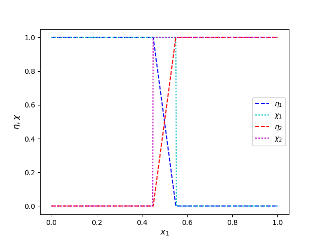
Figure 1: Functions of domain decomposition.

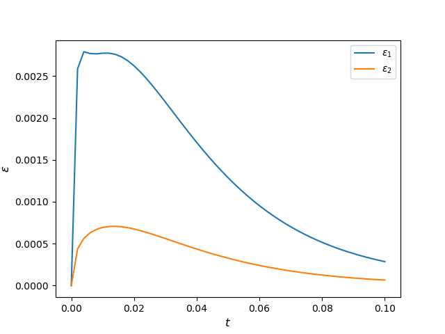
Figure 2: Errors of the domain decomposition schemes.

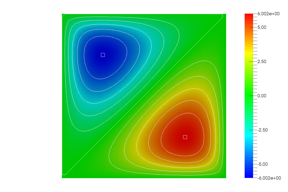
Figure 3: Benchmark solution at the time moment $t=T$.

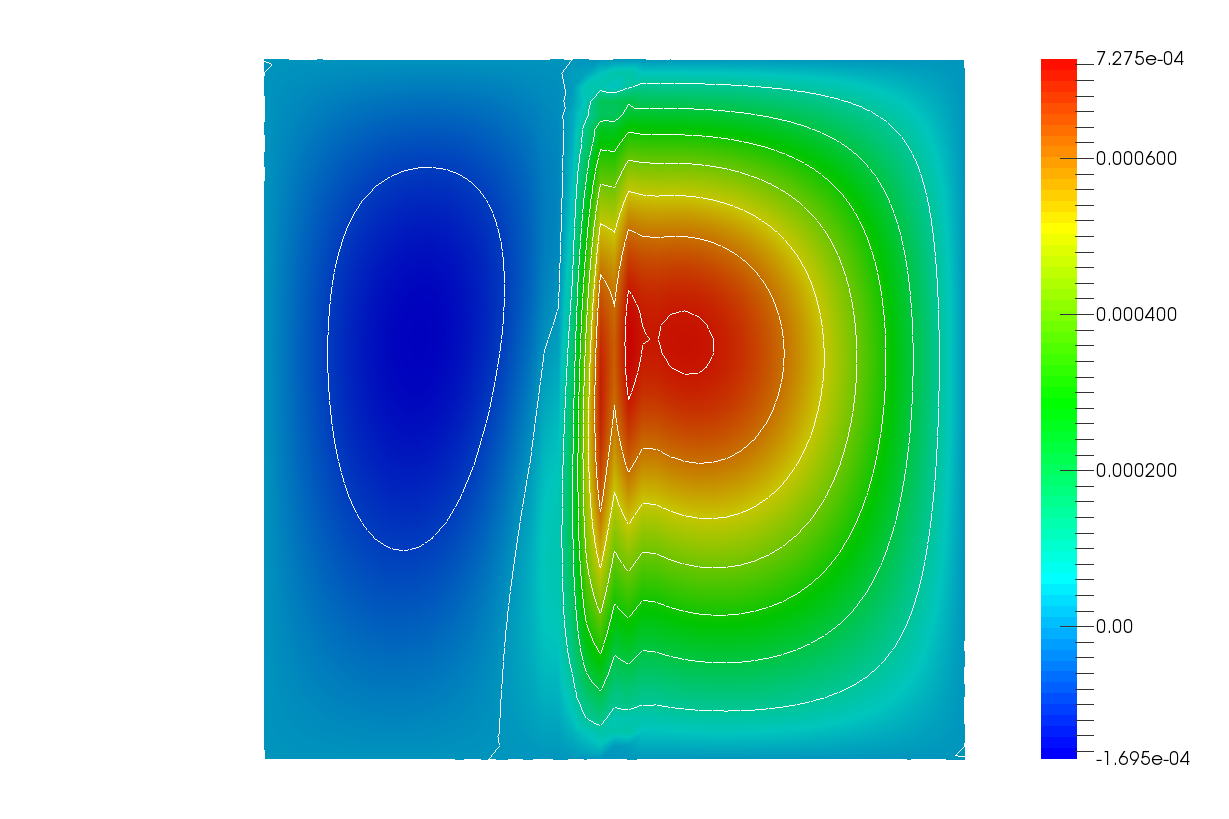
Figure 4: Solution deviation of the scheme based on the partition of unity.

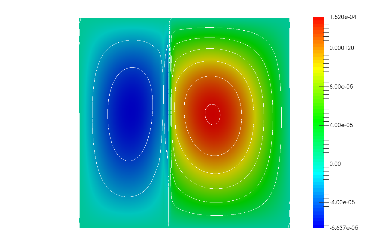
Figure 5: Solution deviation of the scheme based on the indicator functions.

Reducing the overlap width by half (see Fig.6) results in decreasing the accuracy of the approximate solution. For $\delta=0$, both schemes under the consideration coincide and lead to the domain decomposition scheme with non-overlapping subdomains.

The use of a finer grid in space (compare Fig.2 and Fig.7) leads to a drop in accuracy. This fact demonstrates a conditional convergence of the domain decomposition schemes. Calculations with a smaller time step (see Fig.8) allow to increase the accuracy of the numerical solution.

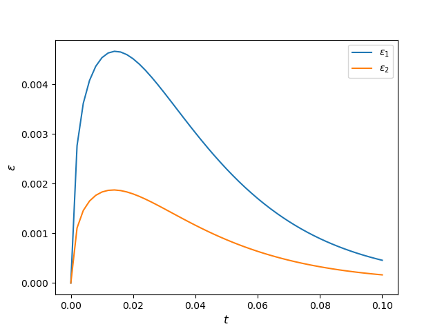
Figure 6: Error of the domain decomposition schemes for $\delta=0.025$.

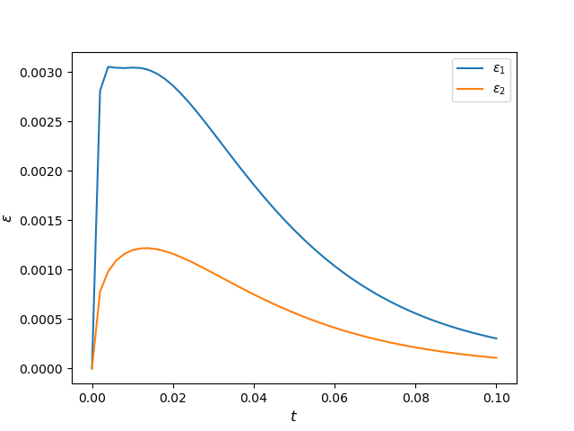
Figure 7: Error of the domain decomposition schemes for the grid $101\times 101$.

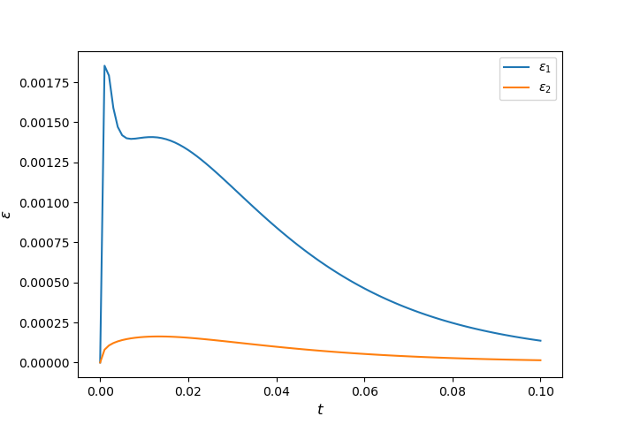
Figure 8: Error of the domain decomposition schemes for $N=100$.

6 Conclusions

The boundary value problem for a second-order parabolic equation is considered. The standard finite element approximation in space is employed. For approximation in time, the two-level scheme with weight ($\theta$-method) is used.

Iteration-free schemes of domain decomposition with overlapping subdomains are constructed on the basis of a partition of unity for a computational domain. In the case of a two-component domain decomposition, approximation in time is designed using factorized schemes, which generalize the standard ADI schemes.

A new class of domain decomposition schemes with overlapping subdomains based on indicator functions of subdomains is proposed for unsteady problems. In this case, for the problem operator, we have a three-component representation with decomposition operators connected with subdomains and their intersection. The unconditional stability of these schemes is established for two-component schemes of domain decomposition.

Numerical results for the model two-dimensional problem demonstrate the robustness of the new decomposition scheme with overlapping subdomains. A comparison of the conventional scheme based on a partition of unity with the scheme that used the indicator functions of the subdomains demonstrates its advantage in accuracy.

References

- Abrashin (1990) Abrashin, V. N., 1990. A variant of the method of variable directions for the solution of multidimensional problems of mathematical-physics. I. Differential equations 26, 314–323, in Russian.
- Abrashin and Vabishchevich (1998) Abrashin, V. N., Vabishchevich, P. N., 1998. Vector additive schemes for evolution equations of second order. Differential equations 34 (12), 1666–1674, in Russian.
- Dryja (1991) Dryja, M., 1991. Substructuring methods for parabolic problems. In: Glowinski, R., Kuznetsov, Y. A., Meurant, G. A., Périaux, J., Widlund, O. (Eds.), Fourth International Symposium on Domain Decomposition Methods for Partial Differential Equations. SIAM, Philadelphia, PA.
- Grossmann et al. (2007) Grossmann, C., Roos, H. G., Stynes, M., 2007. Numerical Treatment of Partial Differential Equations. Springer Verlag.
- Kellogg (1964) Kellogg, R. B., 1964. An alternating direction method for operator equations. Journal of the Society for Industrial and Applied Mathematics 12 (4), 848–854.
- Kuznetsov (1988) Kuznetsov, Y. A., 1988. New algorithms for approximate realization of implicit difference schemes. Sov. J. Numer. Anal. Math. Model. 3 (2), 99–114.
- Kuznetsov (1991) Kuznetsov, Y. A., 1991. Overlapping domain decomposition methods for FE-problems with elliptic singular perturbed operators. Fourth international symposium on domain decomposition methods for partial differential equations, Proc. Symp., Moscow/Russ. 1990, 223-241 (1991).
- Laevsky (1987) Laevsky, Y. M., 1987. Domain decomposition methods for the solution of two-dimensional parabolic equations. In: Variational-difference methods in problems of numerical analysis. No. 2. Comp. Cent. Sib. Branch, USSR Acad. Sci., Novosibirsk, pp. 112–128, in Russian.
- Marchuk (1990) Marchuk, G. I., 1990. Splitting and alternating direction methods. In: Ciarlet, P. G., Lions, J.-L. (Eds.), Handbook of Numerical Analysis, Vol. I. North-Holland, pp. 197–462.
- Mathew et al. (1998) Mathew, T. P., Polyakov, P. L., Russo, G., Wang, J., 1998. Domain decomposition operator splittings for the solution of parabolic equations. SIAM Journal on Scientific Computing 19 (3), 912–932.
- Quarteroni and Valli (1999) Quarteroni, A., Valli, A., 1999. Domain Decomposition Methods for Partial Differential Equations. Clarendon Press.
- Samarskii (1967) Samarskii, A. A., 1967. Regularization of difference schemes. Zh. Vychisl. Mat. Mat. Fiz. 7, 62–93, in Russian.
- Samarskii (2001) Samarskii, A. A., 2001. The Theory of Difference Schemes. Marcel Dekker, New York.
- Samarskii et al. (2002) Samarskii, A. A., Matus, P. P., Vabishchevich, P. N., 2002. Difference Schemes with Operator Factors. Kluwer Academic Pub.
- Samarskii and Vabishchevich (1995) Samarskii, A. A., Vabishchevich, P. N., 1995. Vector additive schemes of domain decomposition for parabolic problems. Differential equations 31, 1563–1569, in Russian.
- Toselli and Widlund (2005) Toselli, A., Widlund, O., 2005. Domain Decomposition Methods – Algorithms and Theory. Springer.
- Vabishchevich (1989) Vabishchevich, P. N., 1989. Difference schemes decompose the computational domain for solving transient problems. Zh. Vychisl. Mat. Mat. Fiz. 29 (12), 1822–1829, in Russian.
- Vabishchevich (1994a) Vabishchevich, P. N., 1994a. Parallel domain decomposition algorithms for time-dependent problems of mathematical physics. In: Advances in Numerical Methods and Applications. World Schientific, pp. 293–299.
- Vabishchevich (1994b) Vabishchevich, P. N., 1994b. Regionally additive difference schemes for stabilizing correction for parabolic problems. Zh. Vychisl. Mat. Mat. Fiz. 34 (12), 1832–1842, in Russian.
- Vabishchevich (1996) Vabishchevich, P. N., 1996. Vector additive difference schemes for second order evolution equations. Zh. Vychisl. Mat. Mat. Fiz. 36(3), 44–51, in Russian.
- Vabishchevich (2008) Vabishchevich, P. N., 2008. Domain decomposition methods with overlapping subdomains for the time-dependent problems of mathematical physics. Computational Methods in Applied Mathematics 8 (4), 393–405.
- Vabishchevich (2011) Vabishchevich, P. N., 2011. A substructuring domain decomposition scheme for unsteady problems. Computational Methods in Applied Mathematics 11 (2), 241–268.
- Vabishchevich (2014) Vabishchevich, P. N., 2014. Additive Operator-Difference Schemes: Splitting Schemes. de Gruyter.