Evolution of tripartite entangled states in a decohering environment and their experimental protection using dynamical decoupling

Abstract

We embarked upon the task of experimental protection of different classes of tripartite entangled states, namely the maximally entangled GHZ and W states and the ${\rm W\bar{W}}$ state, using dynamical decoupling. The states were created on a three-qubit NMR quantum information processor and allowed to evolve in the naturally noisy NMR environment. Tripartite entanglement was monitored at each time instant during state evolution, using negativity as an entanglement measure. It was found that the W state is most robust while the GHZ-type states are most fragile against the natural decoherence present in the NMR system. The ${\rm W\bar{W}}$ state which is in the GHZ-class, yet stores entanglement in a manner akin to the W state, surprisingly turned out to be more robust than the GHZ state. The experimental data were best modeled by considering the main noise channel to be an uncorrelated phase damping channel acting independently on each qubit, alongwith a generalized amplitude damping channel. Using dynamical decoupling, we were able to achieve a significant protection of entanglement for GHZ states. There was a marginal improvement in the state fidelity for the W state (which is already robust against natural system decoherence), while the ${\rm W\bar{W}}$ state showed a significant improvement in fidelity and protection against decoherence.

I Introduction

Quantum entanglement is considered to lie at the crux of QIP Nielsen and Chuang (2000) and while two-qubit entanglement can be completely characterized, multipartite entanglement is more difficult to quantify and is the subject of much recent research Horodecki et al. (2009). Entanglement can be rather fragile under decoherence and various multiparty entangled states behave very differently under the same decohering channel Dur and Briegel (2004). It is hence of paramount importance to understand and control the dynamics of multipartite entangled states in multivarious noisy environments Mintert et al. (2005); Aolita et al. (2008, 2015).

A three-qubit system is a good model system to study the diverse response of multipartite entangled states to decoherence and the entanglement dynamics of three-qubit GHZ and W states were theoretically studied Borras et al. (2009); Weinstein (2010). Under an arbitrary (Markovian) decohering environment, it was shown that W states are more robust than GHZ states for certain kinds of channels while the reverse is true for other kinds of channels Carvalho et al. (2004); Siomau and Fritzsche (2010a, b); Ali and Guhne (2014).

On the experimental front, tripartite entanglement was generated using photonic qubits and the robustness of W state entanglement was studied in optical systems Lanyon and Langford (2009); Zang et al. (2015); He and Yang (2015); Zang et al. (2016). The dynamics of multi-qubit entanglement under the influence of decoherence was experimentally characterized using a string of trapped ions Barreiro et al. (2010) and in superconducting qubits Wu et al. (2016). In the context of NMR quantum information processing, three-qubit entangled states were experimentally prepared Peng et al. (2010); Dogra et al. (2015); Manu and Kumar (2014), and their decay rates compared with bipartite entangled states Kawamura et al. (2006).

With a view to protecting entanglement, dynamical decoupling (DD) schemes have been successfully applied to decouple a multiqubit system from both transverse dephasing and longitudinal relaxation baths Viola (2004); Uhrig (2008); Kuo et al. (2012); Zhen et al. (2016). UDD schemes have been used in the context of entanglement preservation Song et al. (2013); Franco et al. (2014), and it was shown theoretically that Uhrig DD schemes are able to preserve the entanglement of two-qubit Bell states and three-qubit GHZ states for quite long times Agarwal (2010).

In this work, we experimentally explored the robustness against decoherence, of three different tripartite entangled states, namely, the GHZ, W and $\rm W{\bar{W}}$ states. The ${\rm W{\bar{W}}}$ state is a novel tripartite entangled state which belongs to the GHZ entanglement class in the sense that it is SLOCC equivalent to the GHZ state, however stores its entanglement in ways very similar to that of the W state Devi et al. (2012); Das et al. (2015). We created these states with a very high fidelity, via GRAPE-optimized rf pulses Tosner et al. (2009) on a system of three NMR qubits, using three fluorine spins individually addressable in frequency space. We allowed these entangled states to decohere and measured their entanglement content at different instances in time. To estimate the fidelity of state preparation and entanglement content, we performed complete state tomography Leskowitz and Mueller (2004) using maximum likelihood estimation Singh et al. (2016). As a measure for tripartite entanglement, we used a well-known extension of the bipartite Peres-Horodecki separability criterion Peres (1996) called negativity Vidal and Werner (2002).

Our results showed that the W state was most robust against the environmental noise, followed by the ${\rm W{\bar{W}}}$ state, while the GHZ state was rather fragile. We analytically solved the Lindblad master equation for decohering open quantum systems and showed that the best-fit to our experimental data was provided by a model which considered two predominant noise channels acting on the three qubits: and a homogeneous phase-damping channel acting independently on each qubit and a generalized amplitude damping channel. Next, we protected entanglement of these states using two different DD sequences: the symmetrized XY-16(s) and the Knill dynamical decoupling (KDD) sequences, and evaluated their efficacy of protection. Both DD schemes were able to achieve a good degree of entanglement protection. The GHZ state was dramatically protected, with its entanglement persisting for nearly double the time. The W state showed a marginal improvement, which was to be expected since these DD schemes are designed to protect mainly against dephasing noise, and our results indicated that the W state is already robust against this type of decohering channel. Interestingly, although the $\rm W{\bar{W}}$ state belongs to the GHZ entanglement-class, our experiments revealed that its entanglement persists for a longer time than the GHZ state, while the DD schemes are able to preserve its entanglement to a reasonable extent. The decoherence characteristics of the ${\rm W\bar{W}}$ state hence suggest a way of protecting fragile GHZ-type states against noise by transforming the type of entanglement (since a GHZ-class state can be transformed via local operations to a ${\rm W\bar{W}}$ state). These aspects of the entanglement dynamics of the ${\rm W{\bar{W}}}$ state require more detailed studies for a better understanding.

There has been a longstanding debate about the existence of entanglement in spin ensembles at high temperature as encountered in NMR experiments. There are two ways to look at the situation. Entangled states in such ensembles are obtained via unitary transformations on pseudopure states. If we consider the entire spin ensemble, given that the number of spins that are involved in the pseudopure state is very small compared to the total number of spins, it has been shown that the overall ensemble is not entangled Braunstein et al. (1999); Yu et al. (2005). However one can take a different point of view and only consider the sub-ensemble of spins that have been prepared in the pseudopure state, and as far as these spins are concerned, entanglement genuinely exists Soares-Pinto et al. (2012); Serra and Oliveira (2012); Gui-Lu et al. (2002). The states that we have created are entangled in this sense, and hence may not be considered as entangled if one works with the entire ensemble. Therefore, one has to be aware and cautious about this aspect while dealing with these states. These states are sometimes referred to as being pseudo-entangled. Moreover, these states have interesting properties in terms of the presence of multiple-quantum coherences and their evolution and dynamics under decoherence.

This paper is organized as follows: In Section II we describe the experimental decoherence behaviour of tripartite entangled states, with section II.1 containing details of the NMR system section II.2 delineating the experimental schemes to prepare tripartite-entangled GHZ, W and $\rm W{\bar{W}}$ states. The experimental entanglement dynamics of these states decohering in a noisy environment is contained in section II.3. Section III describes the results of protecting these tripartite entangled states using robust dynamical decoupling sequences, while Section IV presents some conclusions. The theoretical model of noise damping used to fit the experimental data is described in the Appendix.

II Dynamics of tripartite entangled states

II.1 Three-qubit NMR system

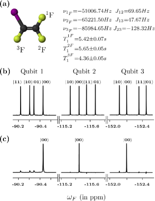
Figure 1: (a) Molecular structure of trifluoroiodoethylene molecule and tabulated system parameters with chemical shifts $\nu_{i}$ and scalar couplings J_ij (in Hz), and spin-lattice relaxation times $T_{1}$ and spin-spin relaxation times T₂ (in seconds). (b) NMR spectrum obtained after a $\pi/2$ readout pulse on the thermal equilibrium state. and (c) NMR spectrum of the pseudopure $|000\rangle$ state. The resonance lines of each qubit are labeled by the corresponding logical states of the other qubit.

We use the three ¹⁹F nuclear spins of the trifluoroiodoethylene (C₂F₃I) molecule to encode the three qubits. On an NMR spectrometer operating at 600 MHz, the fluorine spin resonates at a Larmor frequency of $\approx 564$ MHz. The molecular structure of the three-qubit system with tabulated system parameters and the NMR spectra of the qubits at thermal equilibrium and prepared in the pseudopure state $|000\rangle$ are shown in Figs. 1(a), (b), and (c), respectively. The Hamiltonian of a weakly-coupled three-spin system in a frame rotating at $\omega_{{\rm rf}}$ (the frequency of the electromagnetic field $B_{1}(t)$ applied to manipulate spins in a static magnetic field $B_{0}$) is given by Ernst et al. (1987):

$${\cal H}=-\sum_{i=1}^{3}(\omega_{i}-\omega_{{\rm rf}})I_{iz}+\sum_{i<j,j=1}^{3}2\pi J_{ij}I_{iz}I_{jz}$$ (1)

where $I_{iz}$ is the spin angular momentum operator in the $z$ direction for ¹⁹F; the first term in the Hamiltonian denotes the Zeeman interaction between the fluorine spins and the static magnetic field $B_{0}$ with $\omega_{i}=2\pi\nu_{i}$ being the Larmor frequencies; the second term represents the spin-spin interaction with $J_{ij}$ being the scalar coupling constants. The three-qubit equilibrium density matrix (in the high temperature and high field approximations) is in a highly mixed state given by:

$$\rho_{eq} = \tfrac{1}{8}(I+\epsilon\ \Delta\rho_{eq})$$

$$\Delta\rho_{{\rm eq}} \propto \sum_{i=1}^{3}I_{iz}$$ (2)

with a thermal polarization $\epsilon\sim 10^{-5}$, $I$ being the $8\times 8$ identity operator and $\Delta\rho_{{\rm eq}}$ being the deviation part of the density matrix. The system was first initialized into the $|000\rangle$ pseudopure state using the spatial averaging technique Cory et al. (1998), with the density operator given by

$$\rho_{000}=\frac{1-\epsilon}{8}I+\epsilon|000\rangle\langle 000|$$ (3)

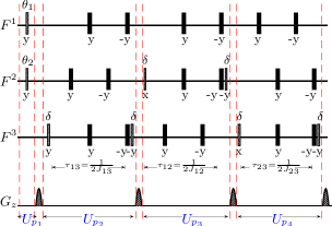
Figure 2: NMR pulse sequence used to prepare pseudopure state $\rho_{000}$ starting from thermal equilibrium.The pulses represented by black filled rectangles are of angle $\pi$. The other rf flip angles are set to $\theta_{1}=\frac{5\pi}{12}$, $\theta_{2}=\frac{\pi}{6}$ and $\delta=\frac{\pi}{4}$. The phase of each rf pulse is written below each pulse bar. The evolution interval $\tau_{ij}$ is set to a multiple of the scalar coupling strength ($J_{ij}$).

The specific sequence of rf pulses, $z$ gradient pulses and time evolution periods we used to prepare the pseudopure state $\rho_{000}$ starting from thermal equilibrium is shown in Figure 2. All the rf pulses used in the pseudopure state preparation scheme were constructed using the Gradient Ascent Pulse Engineering (GRAPE) technique Tosner et al. (2009) and were designed to be robust against rf inhomogeneity, with an average fidelity of $\geq 0.99$. Wherever possible, two independent spin-selective rf pulses were combined using a specially crafted single GRAPE pulse; for instance the first two rf pulses to be applied before the first field gradient pulse, were combined into a single pulse specially crafted pulse ($U_{p_{1}}$ in Figure 2), of duration $600\mu$s. The combined pulses $U_{p_{2}}$, $U_{p_{3}}$ and $U_{p_{4}}$ applied later in the sequence were of a total duration $\approx 20$ ms.

All experimental density matrices were reconstructed using a reduced tomographic protocol and by using maximum likelihood estimation Leskowitz and Mueller (2004); Singh et al. (2016) with the set of operations $\{III,IIY,IYY,YII,XYX,XXY,XXX\}$; $I$ is the identity (do-nothing operation) and $X(Y)$ denotes a single spin operator implemented by a spin-selective $\pi/2$ pulse. We constructed these spin-selective pulses for tomography using GRAPE, with the length of each pulse $\approx 600\mu$s. The fidelity of an experimental density matrix was estimated by measuring the projection between the theoretically expected and experimentally measured states using the Uhlmann${\rm-}$Jozsa fidelity measure Uhlmann (1976); Jozsa (1994):

$$F=\left(Tr\left(\sqrt{\sqrt{\rho_{\rm theory}}\rho_{\rm expt}\sqrt{\rho_{\rm theory}}}\right)\right)^{2}$$ (4)

where $\rho_{\rm theory}$ and $\rho_{\rm expt}$ denote the theoretical and experimental density matrices respectively. The experimental density matrices were reconstructed by repeating each experiment ten times (keeping the temperature fixed at 288 K). The mean of the ten experimentally reconstructed density matrices was used to compute the statistical error in the state fidelity. The experimentally created pseudopure state $|000\rangle$ was tomographed with a fidelity of $0.985\pm 0.015$ and the total time taken to prepare the state was $\approx 60$ ms.

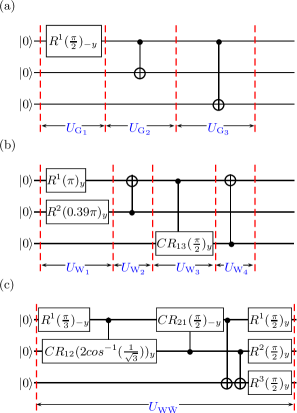
Figure 3: (Quantum circuit showing the sequence of implementation of the single-qubit local rotation gates (labeled by $R$), two-qubit controlled-rotation gates (labeled by $CR$) and controlled-NOT gates required to construct the (a) GHZ state (b) W state and (c) ${\rm W\bar{W}}$ state.

II.2 NMR implementation of tripartite entangled states

Tripartite entanglement has been well characterized and it is known that the two different classes of tripartite entanglement, namely GHZ-class and W-class, are inequivalent. While both classes are maximally entangled, there are differences in the their type of entanglement: the W-class entanglement is more robust against particle loss than the GHZ-class (which becomes separable if one particle is lost) and it is also known that the W state has the maximum possible bipartite entanglement in its reduced two-qubit states Guhne and Toth (2009). The entanglement in the ${\rm W\bar{W}}$ state (which belongs to the GHZ-class of entanglement) shows a surprising result, that it is reconstructible from its reduced two-qubit states (similar to the W-class of states).

We now turn to the construction of tripartite entangled states on the three-qubit NMR system. The quantum circuits to prepare the three qubits in a GHZ-type state, a W state and a ${\rm W\bar{W}}$ state are shown in Figs. 3 (a), (b) and (c), respectively. Several of the quantum gates in these circuits were optimized using the GRAPE algorithm and we were able to achieve a high gate fidelity and smaller pulse lengths.

The GHZ-type $\frac{1}{\sqrt{2}}(|000\rangle-|111\rangle)$ state was prepared from the $|000\rangle$ pseudopure state by a sequence of three quantum gates (labeled as $U_{G_{1}},U_{G_{2}},U_{G_{3}}$ in Fig. 3(a)): first a selective rotation of $\left[\frac{\pi}{2}\right]_{-y}$ on the first qubit, followed by a CNOT₁₂ gate, and finally a CNOT₁₃ gate. The step-by-step sequential gate operation leads to:

$$|000\rangle \stackrel{{\scriptstyle{R^{1}{\left(\frac{\pi}{2}\right)_{-y}}}}}{{\longrightarrow}} \frac{1}{\sqrt{2}}\left(|000\rangle-|100\rangle\right)$$ (5)

$$\stackrel{{\scriptstyle\rm CNOT_{12}}}{{\longrightarrow}} \frac{1}{\sqrt{2}}\left(|000\rangle-|110\rangle\right)$$

$$\stackrel{{\scriptstyle\rm CNOT_{13}}}{{\longrightarrow}} \frac{1}{\sqrt{2}}\left(|000\rangle-|111\rangle\right)$$

All the pulses for the three gates used for GHZ state construction were designed using the GRAPE algorithm and had a fidelity $\geq$ 0.995. The GRAPE pulse duration corresponding to the gate $U_{G_{1}}$ is $600\mu$s, while the $U_{G_{2}}$ and $U_{G_{3}}$ gates had pulse durations of $24$ms. The GHZ-type state was prepared with a fidelity of $0.969\pm 0.013$.

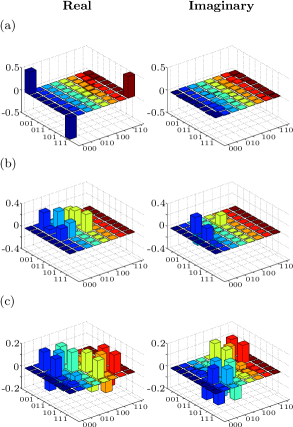
Figure 4: The real (left) and imaginary (right) parts of the experimentally tomographed (a) GHZ-type state, with a fidelity of $0.969\pm 0.013$. (b) W state, with a fidelity of $0.964\pm 0.012$ and (c) $W\bar{W}$ state with a fidelity of $0.937\pm 0.005$. The rows and columns encode the computational basis in binary order from $|000\rangle$ to $|111\rangle$.

The W state was prepared from the initial $|000\rangle$ by a sequence of four unitary operations (labeled as $U_{W_{1}},U_{W_{2}},U_{W_{3}},U_{W_{4}}$ in Fig. 3(b)) and the sequential gate operation leads to:

$$|000\rangle \stackrel{{\scriptstyle R^{1}\left({\pi}\right)_{y}}}{{\longrightarrow}} |100\rangle$$ (6)

$$\stackrel{{\scriptstyle\rm R^{2}\left({0.39\pi}\right)_{y}}}{{\longrightarrow}} \sqrt{\frac{2}{3}}|100\rangle+\frac{1}{\sqrt{3}}|110\rangle$$

$$\stackrel{{\scriptstyle\rm CNOT_{21}}}{{\longrightarrow}} \sqrt{\frac{2}{3}}|100\rangle+\frac{1}{\sqrt{3}}|010\rangle$$

$$\stackrel{{\scriptstyle\rm CR_{13}{\left(\frac{\pi}{2}\right)_{y}}}}{{\longrightarrow}} \frac{1}{\sqrt{3}}[|100\rangle+|101\rangle+|010\rangle]$$

$$\stackrel{{\scriptstyle\rm CNOT_{31}}}{{\longrightarrow}} \frac{1}{\sqrt{3}}[|100\rangle+|001\rangle+|010\rangle]$$

The different unitaries were individually optimized using GRAPE and the pulse duration for $U_{W_{1}}$, $U_{W_{2}}$, $U_{W_{3}}$, and $U_{W_{4}}$ turned out to be $600\mu$s, $24$ms, $16$ms, and $20$ms, respectively and the fidelity of the final state was estimated to be $0.937\pm 0.012$.

The ${\rm W\bar{W}}$ state was constructed by applying the following sequence of gate operations on the $|000\rangle$ state:

$$|000\rangle \stackrel{{\scriptstyle R^{1}\left(\frac{\pi}{3}\right)_{-y}}}{{\longrightarrow}} \frac{\sqrt{3}}{2}|000\rangle-\frac{1}{2}|100\rangle$$ (7)

$$\stackrel{{\scriptstyle\scriptstyle{\rm CR}_{12}\left(0.61\pi\right)_{y}}}{{\longrightarrow}} \frac{\sqrt{3}}{2}|000\rangle-\frac{1}{2\sqrt{3}}|100\rangle-\sqrt{\frac{1}{6}}|110\rangle$$

$$\stackrel{{\scriptstyle\scriptstyle{\rm CR}_{21}\left(\frac{\pi}{2}\right)_{-y}}}{{\longrightarrow}} \frac{1}{2}(\sqrt{3}|000\rangle-\frac{1}{\sqrt{3}}(|100\rangle+|110\rangle+$$

$$|010\rangle))$$

$$\stackrel{{\scriptstyle\rm CNOT_{13}}}{{\longrightarrow}} \frac{1}{2}(\sqrt{3}|000\rangle-\frac{1}{\sqrt{3}}(|101\rangle+|111\rangle+$$

$$|010\rangle))$$

$$\stackrel{{\scriptstyle\rm CNOT_{23}}}{{\longrightarrow}} \frac{1}{2}(\sqrt{3}|000\rangle-\frac{1}{\sqrt{3}}(|101\rangle+|110\rangle+$$

$$|011\rangle))$$

$$\stackrel{{\scriptstyle\rm R^{123}\left(\frac{\pi}{2}\right)_{y}}}{{\longrightarrow}} \frac{1}{\sqrt{6}}(|001\rangle+|010\rangle+|011\rangle+$$

$$|100\rangle+|101\rangle+|110\rangle)$$

The unitary operator for the entire preparation sequence (labeled $U_{W\bar{W}}$ in Fig. 3(c)) comprising a spin-selective rotation operator: two controlled-rotation gates, two controlled-NOT gates and one non-selective rotation by $\frac{\pi}{2}$ on all the three qubits, was created by a specially crafted single GRAPE pulse (of pulse length $48$ms) and applied to the initial state $|000\rangle$. The final state had a computed fidelity of $0.937\pm 0.005$.

II.3 Decay of tripartite entanglement

We next turn to the dynamics of tripartite entanglement under decoherence channels acting on the system. For two qubits, all entangled states are negative under partial transpose (NPT) and for such NPT states, the minimum eigenvalues of the partially transposed density operator is a measure of entanglement Peres (1996). This idea has been extended to three qubits, and entanglement can be quantified for our three-qubit system using the well-known tripartite negativity ${\cal N}^{(3)}_{123}$ measure Vidal and Werner (2002); Weinstein (2010):

$${\cal{N}}^{(3)}_{123}=[{\cal N}_{1}{\cal N}_{2}{\cal N}_{3}]^{1/3}$$ (8)

where the negativity of a qubit ${\cal N}_{i}$ refers to the most negative eigenvalue of the partial transpose of the density matrix with respect to the qubit $i$. We studied the time evolution of the tripartite negativity ${\cal N}^{(3)}_{123}$ for the tripartite entangled states, as computed from the experimentally reconstructed density matrices at each time instant. The experimental results are depicted in Fig 5 (a), (b) and (c) for the GHZ state, the ${\rm W\bar{W}}$ state, and the W state, respectively. Of the three entangled states considered in this study, the GHZ and W states are maximally entangled and hence contain the most amount of tripartite negativity, while the ${\rm W\bar{W}}$ state is not maximally entangled and hence has a lower tripartite negativity value. The experimentally prepared GHZ state initially has a ${\cal N}^{(3)}_{123}$ of 0.96 (quite close to its theoretically expected value of 1.0). The GHZ state decays rapidly, with its negativity approaching zero in 0.55 s. The experimentally prepared ${\rm W\bar{W}}$ state initially has a ${\cal N}^{(3)}_{123}$ of 0.68 (close to its theoretically expected value of 0.74), with its negativity approaching zero at 0.67 s. The experimentally prepared W state initially has a ${\cal N}^{(3)}_{123}$ of 0.90 (quite close to its theoretically expected value of 0.94). The W state is quite long-lived, with its entanglement persisting up to 0.9 s. The tomographs of the experimentally reconstructed density matrices of the GHZ, W and ${\rm W\bar{W}}$ states at the time instances when the tripartite negativity parameter ${\cal N}^{(3)}_{123}$ approaches zero for each state, are displayed in Fig. 6.

We explored the noise channels acting on our three-qubit NMR entangled states which best fit our experimental data, by analytically solving a master equation in the Lindblad form, along the lines suggested in Reference Jung et al. (2008). The master equation is given by Lindblad (1976):

$$\frac{\partial\rho}{\partial t}=-i[H_{s},\rho]+\sum_{i,\alpha}\left[L_{i,\alpha}\rho L_{i,\alpha}^{\dagger}-\frac{1}{2}\{L^{\dagger}_{i,\alpha}L_{i,\alpha},\rho\}\right]$$ (9)

where $H_{s}$ is the system Hamiltonian, $L_{i,\alpha}\equiv\sqrt{\kappa_{i,\alpha}}\sigma^{(i)}_{\alpha}$ is the Lindblad operator acting on the $i$th qubit and $\sigma^{(i)}_{\alpha}$ is the Pauli operator on the $i$th qubit, $\alpha=x,y,z$; the constant $\kappa_{i,\alpha}$ turns out to be the inverse of the decoherence time.

Figure 5: Time dependence of the tripartite negativity ${\cal N}^{(3)}$ for the three-qubit system initially experimentally prepared in the (a) GHZ state (squares) (b) W state (circles) and (c) ${\rm W{\bar{W}}}$ state (triangles) (the superscript ${\rm exp}$ denotes “experimental data”). The fits are the calculated decay of negativity ${\cal N}^{(3)}$ of the GHZ state (solid line), the $W\bar{W}$ state (dashed line) and the W state (dotted-dashed line), under the action of the modeled NMR noise channel (the superscript ${\rm cal}$ denotes “calculated fit”). The W state is most robust against the NMR noise channel, whereas the GHZ state is most fragile.

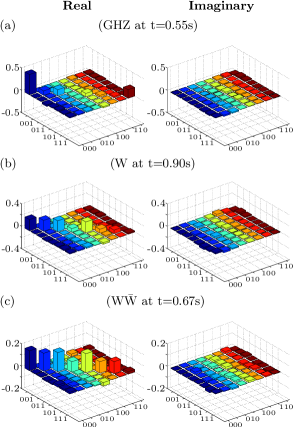
Figure 6: The real (left) and imaginary (right) parts of the the experimentally tomographed density matrix of the state at the time instances when the tripartite negativity ${\cal N}^{(3)}_{123}$ approaches zero for the (a) GHZ state at $t=0.55$ s (b) W state at $t=0.90$ s and (c) ${\rm W\bar{W}}$ state at $t=0.67$ s. The rows and columns encode the computational basis in binary order, from $|000\rangle$ to $|111\rangle$.

We consider a decoherence model wherein a nuclear spin is acted on by two noise channels namely a phase damping channel (described by the T₂ relaxation in NMR) and a generalized amplitude damping channel (described by the T₁ relaxation in NMR) Childs et al. (2001). As the fluorine spins in our three-qubit system have widely differing chemical shifts, we assume that each qubit interacts independently with its own environment. The experimentally determined T₁ NMR relaxation rates are T${}_{1}^{1F}=5.42\pm 0.07$ s, T${}_{1}^{2F}=5.65\pm 0.05$ s and T${}_{1}^{3F}=4.36\pm 0.05$ s, respectively. The T₂ relaxation rates were experimentally measured by first rotating the spin magnetization into the transverse plane by a $90^{\circ}$ rf pulse followed by a delay and fitting the resulting magnetization decay. The experimentally determined T₂ NMR relaxation rates are T${}_{2}^{1F}=0.53\pm 0.02$s, T${}_{2}^{2F}=0.55\pm 0.02$ s, and T${}_{2}^{3F}=0.52\pm 0.02$ s, respectively. We solved the master equation (Eqn. (9)) for the GHZ, W and ${\rm W\bar{W}}$ states with the Lindblad operators $L_{i,x}\equiv\sqrt{\frac{\kappa_{i,x}}{2}}\sigma^{(i)}_{x}$ and $L_{i,z}\equiv\sqrt{\frac{\kappa_{i,z}}{2}}\sigma^{(i)}_{z}$, where $\kappa_{i,x}=\frac{1}{T_{1}^{i}}$ and $\kappa_{i,z}=\frac{1}{T_{2}^{i}}$. With this model, the GHZ state decays at the rate $\gamma^{al}_{GHZ}=6.33\pm 0.06s^{-1}$, and its entanglement approaches zero in 0.53 s. The $W\bar{W}$ state decays at the rate $\gamma^{al}_{W\bar{W}}=5.90\pm 0.10s^{-1}$, and its entanglement approaches zero in 0.50 s. The $W$ state decays at the rate $\gamma^{al}_{W}=4.84\pm 0.07s^{-1}$, and its entanglement approaches zero in 0.62 s. We used the high-temperature approximation (T $\approx\infty$) to model the noise (the experiments were performed at 288 K), and the results of the analytical calculation and the experimental data match well, as shown in Figure 5.

III Protecting three-qubit entanglement via dynamical decoupling

As the tripartite entangled states under investigation are robust against noise to varying extents, we wanted to discover if either the amount of entanglement in these states could be protected or their entanglement could be preserved for longer times, using dynamical decoupling (DD) protection schemes. While DD sequences are effective in decoupling system-environment interactions, often errors in their implementation arise either due to errors in the pulses or errors due to off-resonant driving Suter and Álvarez (2016). Two approaches have been used to design robust DD sequences which are impervious to pulse imperfections: the first approach replaces the $\pi$ rotation pulses with composite pulses inside the DD sequence, while the second approach focuses on optimizing phases of the pulses in the DD sequence. In this work, we use DD sequences that use pulses with phases applied along different rotation axes: the XY-16(s) and the Knill Dynamical Decoupling (KDD) schemes Souza et al. (2012a).

Figure 7: NMR pulse sequence corresponding to (a) XY-16(s) and (b) KDD_xy DD schemes (the superscript 2 implies that the set of pulses inside the bracket is applied twice, to form one cycle of the DD scheme). The pulses represented by black filled rectangles (in both schemes) are of angle $\pi$, and are applied simultaneously on all three qubits (denoted by $F^{i},i=1,2,3$). The angle below each pulse denotes the phase with which it is applied. Each DD cycle is repeated $N$ times, with $N$ large to achieve good system-bath decoupling.

In conventional DD schemes the $\pi$ pulses are applied along one axis (typically $x$) and as a consequence, only the coherence along that axis is well protected. The XY family of DD schemes applies pulses along two perpendicular ($x,y$) axes, which protects coherence equally along both these axes Souza et al. (2012b). The XY-16(s) sequence is constructed by combining an XY-8(s) cycle with its phase-shifted copy, where the (s) denotes the “symmetric” version i.e. the cycle is time-symmetric with respect to its center. The XY-8 cycle is itself created by combining a basic XY-4 cycle with its time-reversed copy. One full unit cycle of the XY-16(s) sequence comprises sixteen $\pi$ pulses interspersed with free evolution time periods, and each cycle is repeated $N$ times for better decoupling. The KDD sequence has additional phases which further symmetrize pulses in the $x-y$ plane and compensate for pulse errors; each $\pi$ pulse in a basic XY DD sequence is replaced by five $\pi$ pulses, each of a different phase Ryan et al. (2010); Souza et al. (2011):

$${\rm KDD}_{\phi}\equiv(\pi)_{\frac{\pi}{6}+\phi}-(\pi)_{\phi}-(\pi)_{\frac{\pi}{2}+\phi}-(\pi)_{\phi}-(\pi)_{\frac{\pi}{6}+\phi}$$ (10)

where $\phi$ denotes the phase of the pulse; we set $\phi=0$ in our experiments. The KDD_ϕ sequence of five pulses given in Eqn. 10 protects coherence along only one axis. To protect coherences along both the $(x,y)$ axes, we use the KDD_xy sequence, which combines two basic five-pulse blocks shifted in phase by $\pi/2$ i.e $[{\rm KDD}_{\phi}-{\rm KDD}_{\phi+\pi/2}]$. One unit cycle of the KDD_xy sequence contains two of these pulse-blocks shifted in phase, for a total of twenty $\pi$ pulses. The XY-16(s) and KDD_xy DD sequences are given in Figs. 7(a) and (b) respectively, where the black filled rectangles represent $\pi$ pulses on all three qubits and $\tau$ ($\tau_{k}$) indicates a free evolution time period. We note here that the chemical shifts of the three fluorine qubits in our particular molecule cover a very large frequency bandwidth, making it difficult to implement an accurate non-selective pulse simultaneously on all the qubits. To circumvent this problem, we crafted a special excitation pulse of duration $\approx 400\mu$s consisting of a set of three Gaussian shaped pulses that are applied at different spin frequency offsets and are frequency modulated to achieve simultaneous excitation Das et al. (2015).

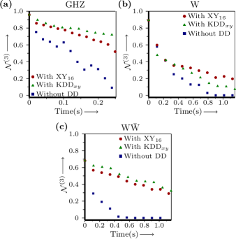
Figure 8: Plot of the tripartite negativity (${\cal N}^{(3)}_{123}$) with time, computed for the (a) GHZ-type state, (b) W state and (c) $W\bar{W}$ state. The negativity was computed for each state without applying any protection and after applying the XY-16(s) and KDD_xy dynamical decoupling sequences.Note that the time scale for part (a) is different from (b) and (c)

Figs.8(a),(b) and (c) show the results of protecting the GHZ, W and ${\rm W\bar{W}}$ states respectively, using the XY-16(s) and the KDD_xy DD sequences.

GHZ state protection: The XY-16(s) protection scheme was implemented on the GHZ state with an inter-pulse delay of $\tau=0.25$ ms and one run of the sequence took $10.40$ ms (including the length of the sixteen $\pi$ pulses). The value of the negativity ${\cal N}^{3}_{123}$ remained close to 0.80 and 0.52 for up to $80$ms and $240$ ms respectively when XY-16 protection was applied, while for the unprotected state the state fidelity is quite low and ${\cal N}^{3}_{123}$ decayed to a low value of 0.58 and 0.09 at $80$ms and $240$ ms, respectively (Fig. 8(a)). The KDD_xy protection scheme on this state was implemented with an inter-pulse delay $\tau_{k}=0.20$ ms and one run of the sequence took $12$ ms (including the length of the twenty $\pi$ pulses). The value of the negativity ${\cal N}^{3}_{123}$ remained close to 0.80 and 0.72 for up to $140$ms and $240$ ms when KDD_xy protection was applied (Fig. 8(a)).

W state protection: The XY-16(s) protection scheme was implemented on the W state with an inter-pulse delay $\tau=3.12$ ms and one run of the sequence took $56.40$ ms (including the length of the sixteen $\pi$ pulses). The value of the negativity ${\cal N}^{3}_{123}$ remained close to 0.30 for up to $0.68$ s when XY-16 protection was applied, whereas ${\cal N}^{3}_{123}$ reduced to 0.1 at $0.68$ s when no state protection is applied (Fig. 8(b)). The KDD_xy protection scheme was implemented on the W state with an inter-pulse delay $\tau_{k}=2.5$ ms and one run of the sequence took $58$ ms (including the length of the twenty $\pi$ pulses). The value of the negativity ${\cal N}^{3}_{123}$ remained close to 0.21 for upto $0.70$ s when KDD_xy protection was applied (Fig. 8(b)).

${\rm W\bar{W}}$ state protection: The XY-16(s) protection sequence was implemented on the ${\rm W\bar{W}}$ state with an inter-pulse delay of $\tau=3.12$ ms and one run of the sequence took $56.40$ ms (including the length of the sixteen $\pi$ pulses). The value of the negativity ${\cal N}^{3}_{123}$ remained close to 0.5 for upto $0.45$ s when XY-16(s) protection was applied, whereas ${\cal N}^{3}_{123}$ reduced almost to zero ($\approx 0.02$) at $0.45$ s when no protection was applied (Fig. 8(c)). The KDD_xy protection sequence was applied with an inter-pulse delay of $\tau_{k}=2.5$ ms and one run of the sequence took $58$ ms (including the length of the twenty $\pi$ pulses). The value of the negativity ${\cal N}^{3}_{123}$ remained close to 0.52 for upto $0.46$ s when KDD_xy protection was applied (Fig. 8(c)).

The results of UDD-type of protection summarized above demonstrate that state protection worked to varying degrees and protected the entanglement of the tripartite entangled states to different extents, depending on the type of state to be protected. The GHZ state showed maximum protection and the ${\rm W\bar{W}}$ state also showed a significant amount of protection, while the W state showed a marginal improvement under protection. We note here that the lifetime of the GHZ state is not significantly enhanced by using DD state protection; what is noteworthy is that state fidelity remains high (close to 0.8) under DD protection, whereas the state quickly gets disentangled (fidelity drops to 0.4) when no protection is applied. This implies that under DD protection, there is no leakage from the state to other states in the Hilbert space of the three qubits.

IV Conclusions

We undertook an experimental study of the dynamics of tripartite entangled states in a three-qubit NMR system. Our results are relevant in the context of other studies which showed that different entangled states exhibit varying degrees of robustness against diverse noise channels. We found that the W state was the most robust against the decoherence channel acting on the three NMR qubits, the GHZ state was the most fragile and decayed very quickly, while the ${\rm W\bar{W}}$ state was more robust than the GHZ state but less robust than the W state. We also implemented entanglement protection on these states using dynamical decoupling sequences. The protection worked to a remarkable extent in entanglement preservation in the GHZ and ${\rm W\bar{W}}$ states, while the W state showed a better fidelity under protection but no appreciable increase in the lifetime of entanglement. The entangled states that we deal with in this study are obtained by unitary transformations on pseudopure states, where only a small subset of spins participate, and are thus pseudo-entangled. Our results have important implications for entanglement storage and preservation in realistic quantum information processing protocols.

*

Appendix A Analytical solution of the Lindblad master equation

We analytically solved a master equation of the Lindblad form given in Eqn. 9 Lindblad (1976); Jung et al. (2008), by putting in explicit values for the Lindblad operators according to the two main NMR noise channels (generalized amplitude damping and phase damping), and computed the decay behavior of the GHZ, W and ${\rm W\bar{W}}$ states.

Under the simultaneous action of all the NMR noise channels, the GHZ state decoheres as:

$$\rho_{GHZ}=\left(\begin{array}[]{cccccccc}\alpha_{1}&0&0&0&0&0&0&\beta_{1}\\ 0&\alpha_{2}&0&0&0&0&\beta_{2}&0\\ 0&0&\alpha_{3}&0&0&\beta_{3}&0&0\\ 0&0&0&\alpha_{4}&\beta_{4}&0&0&0\\ 0&0&0&\beta_{4}&\alpha_{4}&0&0&0\\ 0&0&\beta_{3}&0&0&\alpha_{3}&0&0\\ 0&\beta_{2}&0&0&0&0&\alpha_{2}&0\\ \beta_{1}&0&0&0&0&0&0&\alpha_{1}\\ \end{array}\right)$$ (11)

where

$$\alpha_{1} = \frac{1}{8}(1+e^{-(\kappa_{x,1}+\kappa_{x,2})t}+e^{-(\kappa_{x,1}+\kappa_{x,3})t}+e^{-(\kappa_{x,2}+\kappa_{x,3})t})$$

$$\alpha_{2} = \frac{1}{8}(1+e^{-(\kappa_{x,1}+\kappa_{x,2})t}-e^{-(\kappa_{x,1}+\kappa_{x,3})t}-e^{-(\kappa_{x,2}+\kappa_{x,3})t})$$

$$\alpha_{3} = \frac{1}{8}(1-e^{-(\kappa_{x,1}+\kappa_{x,2})t}+e^{-(\kappa_{x,1}+\kappa_{x,3})t}-e^{-(\kappa_{x,2}+\kappa_{x,3})t})$$

$$\alpha_{4} = \frac{1}{8}(1-e^{-(\kappa_{x,1}+\kappa_{x,2})t}-e^{-(\kappa_{x,1}+\kappa_{x,3})t}+e^{-(\kappa_{x,2}+\kappa_{x,3})t})$$

$$\beta_{1} = \frac{1}{8}(e^{-(\kappa_{1,x}+\kappa_{2,x}+\kappa_{3,x}+\kappa_{1,z}+\kappa_{2,z}+\kappa_{3,z})t}$$

$$\quad(e^{\kappa_{1,x}t}+e^{\kappa_{2,x}t}+e^{\kappa_{3,x}t}+e^{(\kappa_{1,x}+\kappa_{2,x}+\kappa_{3,x})t})$$

$$\beta_{2} = \frac{1}{8}(e^{-(\kappa_{1,x}+\kappa_{2,x}+\kappa_{3,x}+\kappa_{1,z}+\kappa_{2,z}+\kappa_{3,z})t}$$

$$\quad(-e^{\kappa_{1,x}t}-e^{\kappa_{2,x}t}+e^{\kappa_{3,x}t}+e^{(\kappa_{1,x}+\kappa_{2,x}+\kappa_{3,x})t})$$

$$\beta_{3} = \frac{1}{8}(e^{-(\kappa_{1,x}+\kappa_{2,x}+\kappa_{3,x}+\kappa_{1,z}+\kappa_{2,z}+\kappa_{3,z})t}$$

$$(-e^{\kappa_{1,x}t}+e^{\kappa_{2,x}t}-e^{\kappa_{3,x}t}+e^{(\kappa_{1,x}+\kappa_{2,x}+\kappa_{3,x})t})$$

$$\beta_{4} = \frac{1}{8}(e^{-(\kappa_{1,x}+\kappa_{2,x}+\kappa_{3,x}+\kappa_{1,z}+\kappa_{2,z}+\kappa_{3,z})t}$$

$$\quad(e^{\kappa_{1,x}t}-e^{\kappa_{2,x}t}-e^{\kappa_{3,x}t}+e^{(\kappa_{1,x}+\kappa_{2,x}+\kappa_{3,x})t})$$

Under the simultaneous action of all the NMR noise channels, the W state decoheres as:

$$\rho_{W}=\left(\begin{array}[]{cccccccc}\alpha_{1}&0&0&\beta_{1}&0&\beta_{5}&\beta_{1}&0\\ 0&\alpha_{2}&\beta_{2}&0&\beta_{6}&0&0&\beta_{10}\\ 0&\beta_{2}&\alpha_{3}&0&\beta_{11}&0&0&\beta_{7}\\ \beta_{1}&0&0&\alpha_{4}&0&\beta_{12}&\beta_{8}&0\\ 0&\beta_{6}&\beta_{11}&0&\alpha_{5}&0&0&\beta_{3}\\ \beta_{5}&0&0&\beta_{12}&0&\alpha_{6}&\beta_{4}&0\\ \beta_{1}&0&0&\beta_{8}&0&\beta_{4}&\alpha_{7}&0\\ 0&\beta_{10}&\beta_{7}&0&\beta_{3}&0&0&\alpha_{8}\\ \end{array}\right)\\$$

Where

$$\alpha_{1} = \frac{1}{8}-\frac{1}{24}e^{-(\kappa_{x,1}+\kappa_{x,2}+\kappa_{x,3})t}(3+e^{\kappa_{x,1}t}+e^{\kappa_{x,2}t}-$$

$$e^{(\kappa_{x,1}+\kappa_{x,2})t}+e^{\kappa_{x,3}t}-e^{(\kappa_{x,1}+\kappa_{x,3})t}-e^{(\kappa_{x,2}+\kappa_{x,3})t})$$

$$\alpha_{2} = \frac{1}{8}+\frac{1}{24}e^{-(\kappa_{x,1}+\kappa_{x,2}+\kappa_{x,3})t}(3+e^{\kappa_{x,1}t}+e^{\kappa_{x,2}t}-$$

$$e^{(\kappa_{x,1}+\kappa_{x,2})t}-e^{\kappa_{x,3}t}+e^{(\kappa_{x,1}+\kappa_{x,3})t}+e^{(\kappa_{x,2}+\kappa_{x,3})t})$$

$$\alpha_{3} = \frac{1}{8}+\frac{1}{24}e^{-(\kappa_{x,1}+\kappa_{x,2}+\kappa_{x,3})t}(3+e^{\kappa_{x,1}t}-e^{\kappa_{x,2}t}$$

$$+e^{(\kappa_{x,1}+\kappa_{x,2})t}+e^{\kappa_{x,3}t}-e^{(\kappa_{x,1}+\kappa_{x,3})t}+e^{(\kappa_{x,2}+\kappa_{x,3})t})$$

$$\alpha_{4} = \frac{1}{8}-\frac{1}{24}e^{-(\kappa_{x,1}+\kappa_{x,2}+\kappa_{x,3})t}(3+e^{\kappa_{x,1}t}-e^{\kappa_{x,2}t}$$

$$+e^{(\kappa_{x,1}+\kappa_{x,2})t}-e^{\kappa_{x,3}t}+e^{(\kappa_{x,1}+\kappa_{x,3})t}-e^{(\kappa_{x,2}+\kappa_{x,3})t})$$

$$\alpha_{5} = \frac{1}{8}+\frac{1}{24}e^{-(\kappa_{x,1}+\kappa_{x,2}+\kappa_{x,3})t}(3-e^{\kappa_{x,1}t}+e^{\kappa_{x,2}t}$$

$$+e^{(\kappa_{x,1}+\kappa_{x,2})t}+e^{\kappa_{x,3}t}+e^{(\kappa_{x,1}+\kappa_{x,3})t}-e^{(\kappa_{x,2}+\kappa_{x,3})t})$$

$$\alpha_{6} = \frac{1}{8}+\frac{1}{24}e^{-(\kappa_{x,1}+\kappa_{x,2}+\kappa_{x,3})t}(-3+e^{\kappa_{x,1}t}-e^{\kappa_{x,2}t}$$

$$-e^{(\kappa_{x,1}+\kappa_{x,2})t}+e^{\kappa_{x,3}t}+e^{(\kappa_{x,1}+\kappa_{x,3})t}-e^{(\kappa_{x,2}+\kappa_{x,3})t})$$

$$\alpha_{7} = \frac{1}{8}+\frac{1}{24}e^{-(\kappa_{x,1}+\kappa_{x,2}+\kappa_{x,3})t}(-3+e^{\kappa_{x,1}t}+e^{\kappa_{x,2}t}$$

$$+e^{(\kappa_{x,1}+\kappa_{x,2})t}-e^{\kappa_{x,3}t}-e^{(\kappa_{x,1}+\kappa_{x,3})t}-e^{(\kappa_{x,2}+\kappa_{x,3})t})$$

$$\alpha_{8} = \frac{1}{8}-\frac{1}{24}e^{-(\kappa_{x,1}+\kappa_{x,2}+\kappa_{x,3})t}(-3+e^{\kappa_{x,1}t}+e^{\kappa_{x,2}t}$$

$$+e^{(\kappa_{x,1}+\kappa_{x,2})t}+e^{\kappa_{x,3}t}+e^{(\kappa_{x,1}+\kappa_{x,3})t}+e^{(\kappa_{x,2}+\kappa_{x,3})t})$$

$$\beta_{1} = \frac{1}{12}(e^{-(\kappa_{x,1}+\kappa_{x,2}+\kappa_{x,3}+\kappa_{z,2}+\kappa_{z,3})t}$$

$$(1+e^{(\kappa_{x,1})t})(-1+e^{(\kappa_{x,2}+\kappa_{x,3})t}))$$

$$\beta_{2} = \frac{1}{12}(e^{-(\kappa_{x,1}+\kappa_{x,2}+\kappa_{x,3}+\kappa_{z,2}+\kappa_{z,3})t}$$

$$(1+e^{(\kappa_{x,1})t})(1+e^{(\kappa_{x,2}+\kappa_{x,3})t}))$$

$$\beta_{3} = \frac{1}{12}(e^{-(\kappa_{x,1}+\kappa_{x,2}+\kappa_{x,3}+\kappa_{z,2}+\kappa_{z,3})t}$$

$$(-1+e^{(\kappa_{x,1})t})(-1+e^{(\kappa_{x,2}+\kappa_{x,3})t}))$$

$$\beta_{4} = \frac{1}{12}(e^{-(\kappa_{x,1}+\kappa_{x,2}+\kappa_{x,3}+\kappa_{z,2}+\kappa_{z,3})t}$$

$$(-1+e^{(\kappa_{x,1})t})(1+e^{(\kappa_{x,2}+\kappa_{x,3})t}))$$

$$\beta_{5} = \frac{1}{12}(e^{-(\kappa_{x,1}+\kappa_{x,2}+\kappa_{x,3}+\kappa_{z,1}+\kappa_{z,3})t}$$

$$(1+e^{(\kappa_{x,2})t})(-1+e^{(\kappa_{x,1}+\kappa_{x,3})t}))$$

$$\beta_{6} = \frac{1}{12}(e^{-(\kappa_{x,1}+\kappa_{x,2}+\kappa_{x,3}+\kappa_{z,1}+\kappa_{z,3})t}$$

$$(1+e^{(\kappa_{x,2})t})(1+e^{(\kappa_{x,1}+\kappa_{x,3})t}))$$

$$\beta_{7} = \frac{1}{12}(e^{-(\kappa_{x,1}+\kappa_{x,2}+\kappa_{x,3}+\kappa_{z,1}+\kappa_{z,3})t}$$

$$(-1+e^{(\kappa_{x,2})t})(-1+e^{(\kappa_{x,1}+\kappa_{x,3})t}))$$

$$\beta_{8} = \frac{1}{12}(e^{-(\kappa_{x,1}+\kappa_{x,2}+\kappa_{x,3}+\kappa_{z,1}+\kappa_{z,3})t}$$

$$(-1+e^{(\kappa_{x,2})t})(1+e^{(\kappa_{x,1}+\kappa_{x,3})t}))$$

$$\beta_{9} = \frac{1}{12}(e^{-(\kappa_{x,1}+\kappa_{x,2}+\kappa_{x,3}+\kappa_{z,1}+\kappa_{z,2})t}$$

$$(-1+e^{(\kappa_{x,1}+\kappa_{x,2})t})(1+e^{(\kappa_{x,3})t}))$$

$$\beta_{10} = \frac{1}{12}(e^{-(\kappa_{x,1}+\kappa_{x,2}+\kappa_{x,3}+\kappa_{z,1}+\kappa_{z,2})t}$$

$$(-1+e^{(\kappa_{x,1}+\kappa_{x,2})t})(-1+e^{(\kappa_{x,3})t}))$$

$$\beta_{11} = \frac{1}{12}(e^{-(\kappa_{x,1}+\kappa_{x,2}+\kappa_{x,3}+\kappa_{z,1}+\kappa_{z,2})t}$$

$$(1+e^{(\kappa_{x,1}+\kappa_{x,2})t})(1+e^{(\kappa_{x,3})t}))$$

$$\beta_{12} = \frac{1}{12}(e^{-(\kappa_{x,1}+\kappa_{x,2}+\kappa_{x,3}+\kappa_{z,1}+\kappa_{z,2})t}$$ (13)

$$(1+e^{(\kappa_{x,1}+\kappa_{x,2})t})(-1+e^{(\kappa_{x,3})t}))$$

Under the simultaneous action of all the NMR noise channels, the ${\rm W\bar{W}}$ state decoheres as:

$$\rho_{{\rm W\bar{W}}}=\left(\begin{array}[]{cccccccc}\alpha_{1}&\beta_{1}&\beta_{2}&\beta_{3}&\beta_{4}&\beta_{5}&\beta_{6}&\beta_{7}\\ \beta_{1}&\alpha_{2}&\beta_{8}&\beta_{9}&\beta_{10}&\beta_{11}&\beta_{12}&\beta_{13}\\ \beta_{2}&\beta_{8}&\alpha_{3}&\beta_{14}&\beta_{15}&\beta_{16}&\beta_{11}&\beta_{5}\\ \beta_{3}&\beta_{9}&\beta_{14}&\alpha_{4}&\beta_{17}&\beta_{15}&\beta_{10}&\beta_{4}\\ \beta_{4}&\beta_{10}&\beta_{15}&\beta_{17}&\alpha_{4}&\beta_{15}&\beta_{9}&\beta_{18}\\ \beta_{5}&\beta_{11}&\beta_{16}&\beta_{15}&\beta_{15}&\alpha_{3}&\beta_{8}&\beta_{2}\\ \beta_{6}&\beta_{12}&\beta_{11}&\beta_{10}&\beta_{9}&\beta_{8}&\alpha_{2}&\beta_{1}\\ \beta_{7}&\beta_{13}&\beta_{5}&\beta_{4}&\beta_{18}&\beta_{2}&\beta_{1}&\alpha_{1}\\ \end{array}\right)$$ (14)

where

$$\alpha_{1} = \frac{1}{24}(3-e^{-(\kappa_{x,1}+\kappa_{x,2})t}-e^{-(\kappa_{x,1}+\kappa_{x,3})t}$$

$$-e^{-(\kappa_{x,2}+\kappa_{x,3})t})$$

$$\alpha_{2} = \frac{1}{24}(3-e^{-(\kappa_{x,1}+\kappa_{x,2})t}+e^{-(\kappa_{x,1}+\kappa_{x,3})t}$$

$$+e^{-(\kappa_{x,2}+\kappa_{x,3})t})$$

$$\alpha_{3} = \frac{1}{24}(3+e^{-(\kappa_{x,1}+\kappa_{x,2})t}-e^{-(\kappa_{x,1}+\kappa_{x,3})t}$$

$$+e^{-(\kappa_{x,2}+\kappa_{x,3})t})$$

$$\alpha_{4} = \frac{1}{24}(3+e^{-(\kappa_{x,1}+\kappa_{x,2})t}+e^{-(\kappa_{x,1}+\kappa_{x,3})t}$$

$$-e^{-(\kappa_{x,2}+\kappa_{x,3})t})$$

$$\beta_{1} = \frac{1}{12}e^{-(\kappa_{x,1}+\kappa_{x,2}+2\kappa_{z,3})t}$$

$$(e^{(\kappa_{x,1}+\kappa_{x,2}+\kappa_{z,3})t}-e^{\kappa_{z,3}t})$$

$$\beta_{2} = \frac{1}{12}e^{-(\kappa_{x,1}+\kappa_{x,3}+2\kappa_{z,2})t}$$

$$(e^{(\kappa_{x,1}+\kappa_{x,3}+\kappa_{z,2})t}-e^{\kappa_{z,2}t})$$

$$\beta_{3} = \frac{1}{12}e^{-(\kappa_{x,2}+\kappa_{x,3}+2(\kappa_{z,2}+\kappa_{z,3}))t}$$

$$(e^{(\kappa_{x,2}+\kappa_{x,3}+\kappa_{z,2}+\kappa_{z,3})t}-e^{(\kappa_{z,2}+\kappa_{z,3})t})$$

$$\beta_{4} = \frac{1}{12}e^{-(\kappa_{x,2}+\kappa_{x,3}+2\kappa_{z,1})t}$$

$$(-e^{\kappa_{z,1}t}+e^{(\kappa_{x,2}+\kappa_{x,3}+\kappa_{z,1})t})$$

$$\beta_{5} = \frac{1}{12}e^{-(\kappa_{x,1}+\kappa_{x,3}+2(\kappa_{z,1}+\kappa_{z,3}))t}$$

$$(-e^{(\kappa_{z,1}+\kappa_{z,3})t}+e^{(\kappa_{x,1}+\kappa_{x,3}+\kappa_{z,1}+\kappa_{z,3})t})$$

$$\beta_{6} = \frac{1}{12}e^{-(\kappa_{x,1}+\kappa_{x,2}+2(\kappa_{z,1}+\kappa_{z,2}))t}$$

$$(-e^{(\kappa_{z,1}+\kappa_{z,2})t}+e^{(\kappa_{x,1}+\kappa_{x,2}+\kappa_{z,1}+\kappa_{z,2})t})$$

$$\beta_{7} = -\frac{1}{24}e^{-(\kappa_{x,1}+\kappa_{x,2}+\kappa_{x,3}+\kappa_{z,1}+\kappa_{z,2}+\kappa_{z,3})t}$$

$$(e^{\kappa_{x,1}t}+e^{\kappa_{x,2}t}+e^{\kappa_{x,3}t}-3e^{(\kappa_{x,1}+\kappa_{x,2}+\kappa_{x,3})t})$$

$$\beta_{8} = \frac{1}{12}e^{-(\kappa_{x,2}+\kappa_{x,3}+2(\kappa_{z,2}+\kappa_{z,3}))t}$$

$$(e^{(\kappa_{z,2}+\kappa_{z,3})t}+e^{(\kappa_{x,2}+\kappa_{x,3}+\kappa_{z,2}+\kappa_{z,3})t})$$

$$\beta_{9} = \frac{1}{12}e^{-(\kappa_{x,1}+\kappa_{x,3}+2\kappa_{z,2})t}$$

$$(e^{\kappa_{z,2}t}+e^{(\kappa_{x,1}+\kappa_{x,3}+\kappa_{z,2})t})$$

$$\beta_{10} = \frac{1}{12}e^{-(\kappa_{x,1}+\kappa_{x,3}+2(\kappa_{z,1}+\kappa_{z,3}))t}$$

$$(e^{(\kappa_{z,1}+\kappa_{z,3})t}+e^{(\kappa_{x,1}+\kappa_{x,3}+\kappa_{z,1}+\kappa_{z,3})t})$$

$$\beta_{11} = \frac{1}{12}e^{-(\kappa_{x,2}+\kappa_{x,3}+2\kappa_{z,1})t}(e^{\kappa_{z,1}t}+e^{(\kappa_{x,2}+\kappa_{x,3}+\kappa_{z,1})t})$$

$$\beta_{12} = \frac{1}{24}e^{-(\kappa_{x,1}+\kappa_{x,2}+\kappa_{x,3}+\kappa_{z,1}+\kappa_{z,2}+\kappa_{z,3})t}$$

$$(e^{\kappa_{x,1}t}+e^{\kappa_{x,2}t}-e^{\kappa_{x,3}t}+3e^{(\kappa_{x,1}+\kappa_{x,2}+\kappa_{x,3})t})$$

$$\beta_{13} = \frac{1}{12}e^{-(\kappa_{x,1}+\kappa_{x,2}+2(\kappa_{z,1}+\kappa_{z,2}))t}$$

$$(-e^{(\kappa_{z,1}+\kappa_{z,2})t}+e^{(\kappa_{x,1}+\kappa_{x,2}+\kappa_{z,1}+\kappa_{z,2})t})$$

$$\beta_{14} = \frac{1}{12}e^{-(\kappa_{x,1}+\kappa_{x,2}+2\kappa_{z,3})t}$$

$$(e^{\kappa_{z,3}t}+e^{(\kappa_{x,1}+\kappa_{x,2}+\kappa_{z,3})t})$$

$$\beta_{15} = \frac{1}{12}e^{-(\kappa_{x,1}+\kappa_{x,2}+2(\kappa_{z,1}+\kappa_{z,2}))t}$$

$$(e^{(\kappa_{z,1}+\kappa_{z,2})t}+e^{(\kappa_{x,1}+\kappa_{x,2}+\kappa_{z,1}+\kappa_{z,2})t})$$

$$\beta_{16} = \frac{1}{24}e^{-(\kappa_{x,1}+\kappa_{x,2}+\kappa_{x,3}+\kappa_{z,1}+\kappa_{z,2}+\kappa_{z,3})t}$$

$$(e^{\kappa_{x,1}t}-e^{\kappa_{x,2}t}+e^{\kappa_{x,3}t}+3e^{(\kappa_{x,1}+\kappa_{x,2}+\kappa_{x,3})t})$$

$$\beta_{17} = \frac{1}{24}e^{-(\kappa_{x,1}+\kappa_{x,2}+\kappa_{x,3}+\kappa_{z,1}+\kappa_{z,2}+\kappa_{z,3})t}$$

$$(-e^{\kappa_{x,1}t}+e^{\kappa_{x,2}t}+e^{\kappa_{x,3}t}+3e^{(\kappa_{x,1}+\kappa_{x,2}+\kappa_{x,3})t})$$

$$\beta_{18} = \frac{1}{12}e^{-(\kappa_{x,2}+\kappa_{x,3}+2(\kappa_{z,2}+\kappa_{z,3}))t}$$ (15)

$$(e^{(\kappa_{z,2}+\kappa_{z,3})t}+e^{(\kappa_{x,2}+\kappa_{x,3}+\kappa_{z,2}+\kappa_{z,3})t})$$

Solving the master equation (Eqn. 9) ensures that the off-diagonal elements of the corresponding $\rho$ matrices satisfy a set of coupled equations, from which the explicit values of $\alpha$s and $\beta$s can be computed. The equations are solved in the high-temperature limit. For an ensemble of NMR spins at room temperature this implies that the energy $E<<k_{B}T$ where $k_{B}$ is the Boltzmann constant and $T$ refers to the temperature, ensuring a Boltzmann distribution of spin populations at thermal equilibrium.

References

- Nielsen and Chuang (2000) M. A. Nielsen and I. L. Chuang, Quantum Computation and Quantum Information (Cambridge University Press, Cambridge UK, 2000).
- Horodecki et al. (2009) R. Horodecki, P. Horodecki, M. Horodecki, and K. Horodecki, Rev. Mod. Phys. 81, 865 (2009).
- Dur and Briegel (2004) W. Dur and H.-J. Briegel, Phys. Rev. Lett. 92, 180403 (2004).
- Mintert et al. (2005) F. Mintert, A. Carvalho, M. Kuś, and A. Buchleitner, Phys. Rep. 415, 207 (2005).
- Aolita et al. (2008) L. Aolita, R. Chaves, D. Cavalcanti, A. Acín, and L. Davidovich, Phys. Rev. Lett. 100, 080501 (2008).
- Aolita et al. (2015) L. Aolita, F. d. Melo, and L. Davidovich, Rep. Prog. Phys. 78, 042001 (2015).
- Borras et al. (2009) A. Borras, A. P. Majtey, A. R. Plastino, M. Casas, and A. Plastino, Phys. Rev. A 79, 022108 (2009).
- Weinstein (2010) Y. S. Weinstein, Phys. Rev. A 82, 032326 (2010).
- Carvalho et al. (2004) A. R. R. Carvalho, F. Mintert, and A. Buchleitner, Phys. Rev. Lett. 93, 230501 (2004).
- Siomau and Fritzsche (2010a) M. Siomau and S. Fritzsche, Eur. Phys. J. D. 60, 397 (2010a).
- Siomau and Fritzsche (2010b) M. Siomau and S. Fritzsche, Phys. Rev. A 82, 062327 (2010b).
- Ali and Guhne (2014) M. Ali and O. Guhne, J. Phys. B 47, 055503 (2014).
- Lanyon and Langford (2009) B. P. Lanyon and N. K. Langford, New. J. Phys. 11, 013008 (2009).
- Zang et al. (2015) X.-P. Zang, M. Yang, F. Ozaydin, W. Song, and Z.-L. Cao, Scientific Reports 5, 16245 (2015).
- He and Yang (2015) X.-L. He and C.-P. Yang, Quantum Inf. Process. 14, 4461 (2015).
- Zang et al. (2016) X.-P. Zang, M. Yang, F. Ozaydin, W. Song, and Z.-L. Cao, Optics Express 24, 12293 (2016).
- Barreiro et al. (2010) J. T. Barreiro, P. Schindler, O. Guhne, T. Monz, M. C., C. F. Roos, M. Hennrich, and R. Blatt, Nature 6, 943 (2010).
- Wu et al. (2016) J. Wu, C. Song, J. Xu, L. Yu, X. Ji, and S. Zhang, Quantum Inf. Process. 15, 3663 (2016).
- Peng et al. (2010) X. Peng, J. Zhang, J. Du, and D. Suter, Phys. Rev. A 81, 042327 (2010).
- Dogra et al. (2015) S. Dogra, K. Dorai, and Arvind, Phys. Rev. A 91, 022312 (2015).
- Manu and Kumar (2014) V. S. Manu and A. Kumar, Phys. Rev. A 89, 052331 (2014).
- Kawamura et al. (2006) M. Kawamura, T. Morimoto, Y. Mori, R. Sawae, K. Takarabe, and Y. Manmoto, Intl. J. Quant. Chem. 106, 3108 (2006).
- Viola (2004) L. Viola, J. Mod. Opt. 51, 2357 (2004).
- Uhrig (2008) G. S. Uhrig, New. J. Phys. 10, 083024 (2008).
- Kuo et al. (2012) W. J. Kuo, G. Quiroz, G. A. Paz-Silva, and D. A. Lidar, J. Math. Phys. 53, 122207 (2012).
- Zhen et al. (2016) X.-L. Zhen, F.-H. Zhang, G. Feng, H. Li, and G.-L. Long, Phys. Rev. A 93, 022304 (2016).
- Song et al. (2013) H. Song, Y. Pan, and Z. Xi, Intl. J. Quant. Infor. 11, 1350012 (2013).
- Franco et al. (2014) R. L. Franco, A. D’Arrigo, G. Falci, G. Compagno, and E. Paladino, Phys. Rev. B 90, 054304 (2014).
- Agarwal (2010) G. S. Agarwal, Physica Scripta 82, 038103 (2010).
- Devi et al. (2012) A. R. U. Devi, Sudha, and A. K. Rajagopal, Quantum Inf. Process. 11, 685 (2012).
- Das et al. (2015) D. Das, S. Dogra, K. Dorai, and Arvind, Phys. Rev. A 92, 022307 (2015).
- Tosner et al. (2009) Z. Tosner, T. Vosegaard, C. Kehlet, N. Khaneja, S. J. Glaser, and N. C. Nielsen, J. Magn. Reson. 197, 120 (2009).
- Leskowitz and Mueller (2004) G. M. Leskowitz and L. J. Mueller, Phys. Rev. A 69, 052302 (2004).
- Singh et al. (2016) H. Singh, Arvind, and K. Dorai, Phys. Lett. A 380, 3051 (2016).
- Peres (1996) A. Peres, Phys. Rev. Lett. 77, 1413 (1996).
- Vidal and Werner (2002) G. Vidal and R. F. Werner, Phys. Rev. A 65, 032314 (2002).
- Braunstein et al. (1999) S. L. Braunstein, C. M. Caves, R. Jozsa, N. Linden, S. Popescu, and R. Schack, Phys. Rev. Lett. 83, 1054 (1999).
- Yu et al. (2005) T. M. Yu, K. R. Brown, and I. L. Chuang, Phys. Rev. A 71, 032341 (2005).
- Soares-Pinto et al. (2012) D. O. Soares-Pinto, R. Auccaise, J. Maziero, A. Gavini-Viana, R. M. Serra, and L. C. Céleri, Philosophical Transactions of the Royal Society of London A: Mathematical, Physical and Engineering Sciences 370, 4821 (2012).
- Serra and Oliveira (2012) R. M. Serra and I. S. Oliveira, Philosophical Transactions of the Royal Society of London A: Mathematical, Physical and Engineering Sciences 370, 4615 (2012).
- Gui-Lu et al. (2002) L. Gui-Lu, Y. Hai-Yang, L. Yan-Song, T. Chang-Cun, Z. Sheng-Jiang, R. Dong, S. Yang, T. Jia-Xun, and C. Hao-Ming, Communications in Theoretical Physics 38, 305 (2002).
- Ernst et al. (1987) R. R. Ernst, G. Bodenhausen, and A. Wokaun, Principles of nuclear magnetic resonance in one and two dimensions (Oxford University Press, New York, 1987).
- Cory et al. (1998) D. Cory, M. Price, and T. Havel, Physica D 120, 82 (1998).
- Uhlmann (1976) A. Uhlmann, Rep. Math. Phys. 9, 273 (1976).
- Jozsa (1994) R. Jozsa, J. Mod. Opt. 41, 2315 (1994).
- Guhne and Toth (2009) O. Guhne and G. Toth, Physics Reports 474, 1 (2009).
- Jung et al. (2008) E. Jung, M.-R. Hwang, Y. H. Ju, M.-S. Kim, S.-K. Yoo, H. Kim, D. Park, J.-W. Son, S. Tamaryan, and S.-K. Cha, Phys. Rev. A 78, 012312 (2008).
- Lindblad (1976) G. Lindblad, Commun. Math. Phys. 48, 119 (1976).
- Childs et al. (2001) A. M. Childs, I. L.Chuang, and D. W. Leung, Phys. Rev. A 64, 012314 (2001).
- Suter and Álvarez (2016) D. Suter and G. A. Álvarez, Rev. Mod. Phys. 88, 041001 (2016).
- Souza et al. (2012a) A. M. Souza, G. A. Alvarez, and D. Suter, Phys. Rev. A 85, 032306 (2012a).
- Souza et al. (2012b) A. M. Souza, G. A. Alvarez, and D. Suter, Phil. T. Roy. Soc. A 370, 4748 (2012b).
- Ryan et al. (2010) C. A. Ryan, J. S. Hodges, and D. G. Cory, Phys. Rev. Lett. 105, 200402 (2010).
- Souza et al. (2011) A. M. Souza, G. A. Alvarez, and D. Suter, Phys. Rev. Lett. 106, 240501 (2011).