-symmetric rational Calogero model with balanced loss and gain
Visva-Bharati University,
Santiniketan, PIN 731 235, India.)
Abstract
A two body rational Calogero model with balanced loss and gain is investigated. The system yields a Hamiltonian which is symmetric under the combined operation of parity () and time reversal () symmetry. It is shown that the system is integrable and exact, stable classical solutions are obtained for particular ranges of the parameters. The corresponding quantum system admits bound state solutions for exactly the same ranges of the parameters for which the classical solutions are stable. The eigen spectra of the system is presented with a discussion on the normalization of the wave functions in proper Stokes wedges. Finally, the Calogero model with balanced loss and gain is studied classically, when the pair-wise harmonic interaction term is replaced by a common confining harmonic potential. The system admits stable solutions for particular ranges of the parameters. However, the integrability and/or exact solvability of the system is obscure due to the presence of the loss and gain terms. The perturbative solutions are obtained and are compared with the numerical results.
keywords: Calogero model, symmetry, Balanced loss and gain.
1 Introduction
The damped harmonic oscillator with a friction term linear in velocity is not a Hamiltonian system. In order to make the system Hamiltonian one needs to introduce a time reversed version of the original oscillator which may be considered as a thermal bath[1]. A system consisting of these two oscillators considered together yields a symmetric Hamiltonian and the total energy is conserved. The Hamiltonian formulation necessarily implies that loss and gain are equally balanced. The quantization of this kind of coupled oscillators having balanced loss and gain is also discussed in the literature[2][3][4][5]. Neither classically stable solutions nor quantum bound states can be obtained for this system. However, the situation changes significantly if these two oscillators are coupled through interactions which are symmetric. An investigation in this regard has been carried out recently[6][7], where a system of coupled oscillators having balanced loss and gain is considered. Both classically stable solutions as well as quantum bound states are obtained within the unbroken symmetric region. Further, this system exhibits symmetric phase transitions which occur at the same ranges of coupling parameter for the classical as well as quantum cases. This mathematical model is motivated by an experiment performed on two coupled -symmetric whispering-gallery-mode optical resonators[8]. The results of this experiment are well explained by the model considered in Ref.[6].
The oscillator systems having balanced loss and gain with different types of couplings are studied extensively in the literature. For example, a pair of mutually coupled active LCR circuits, one with amplification and the other with equivalent attenuation, is used to realize the -symmetric phase transition[9]. A chain of linearly coupled oscillators with its continuum limit is considered in[10]. Further, -symmetric dimer of coupled nonlinear oscillators with cubic nonlinearities is considered in [11]. The system is not amenable to Hamiltonian formulation. Subsequently, a Hamiltonian system of nonlinear oscillators with balanced loss and gain is considered in[12]. The small amplitude oscillations in this system are shown to be governed by a symmetric nonlinear Schrodinger dimer. The common feature of all of these systems is that the unbroken -symmetric regime content classically stable solutions.
The Calogero model [13][14][15][16][17][18] is an exactly solvable model in one dimension where each particle interacts with all other via a long range inverse square potential. There are reviews[19][20][21][22] on the topic discussing various aspects of this model. The Calogero type of systems have its influences in diverse branches of physics such as in exclusion statistics[23], quantum chaos[24],[25], spin chains[26][27] algebraic and integrable structure[28][29], self-adjoint extensions[30][31][32][33], collective field formulation of many-particle systems[34][35] etc.. Therefore, the effect of Calogero type of potential in case of coupled oscillator system having balanced loss and gain is an obvious curiosity. One of our main objectives in this work is to examine how the integrable properties of the Calogero model get modified due to the presence of balanced loss and gain terms. Another motivation of our study is to investigate symmetric phase transition in the presence of specified type of nonlinear interaction governed by inverse square potential. Finally, it is expected that the additional inverse square interaction term may be realized in the context of whispering-gallery-mode optical resonators.
In this article, we investigate a two body rational Calogero model with balanced loss and gain. The system yields a Hamiltonian which is symmetric. We obtain exact stable classical solutions for the particular ranges of the parameters for which the symmetry remains unbroken. A quantization of this classical model is carried out. This quantized version admits bound state solutions for exactly the same ranges of the parameters for which the classical solutions are stable. The eigen spectra and eigen states of the system are presented. The eigen functions are not normalizable along the real line. We define the proper Stoke wedges and discuss the normalization of the ground state wave function in this Stokes wedges. Finally, the Calogero model with balanced loss and gain is studied classically, when the pair-wise harmonic interaction term is replaced by a common confining harmonic potential. In this case the system admits stable solutions in the unbroken symmetric regime. However, the exact solvability of the system is obscure due to the presence of the loss and gain terms. For this case we obtained perturbative solutions in the unbroken () symmetric regime. This perturbative results are compared with the exact numerical calculations.
The plan of this paper is as follows. In the next section we introduce the main model. In section 2.1, we discuss the classical results for a two body rational Calogero model with balanced loss and gain. The exact stable solution for this system is obtained. In section 2.2 , the classical perturbative solutions for the Calogero model with balanced loss and gain are discussed when the pair-wise harmonic interaction term is replaced by a common confining harmonic potential. These results are compared with the numerical calculations. In section 3, the quantum case for two body rational Calogero model with balanced loss and gain is considered. In the last section we make a summary and discuss the results.
2 Classical model
The model we consider has the following Lagrangian:
| (1) |
where the dot over the variables denotes derivative with respect to time. The first four terms describe a pair of two oscillators, having common frequency , with balanced loss and gain and are coupled linearly via coupling parameter . The last term is the reminiscent of the two-body Calogero potential describing a system of two particles interacting with each other via long range inverse square potential. Thus the Lagrangian of Eq. (1) describes a dissipative harmonic oscillator system along with its time reversed version interacting with each other via a two-body inverse square potential plus a linear interacting term. The whole system yields a Hamiltonian
| (2) |
where
| (3) |
are respectively the momenta conjugate to the and variables. The total energy of the system is conserved.
The following Eqs. of motions may be obtained either from the Lagrangian (1) or from the Hamiltonian (2):
| (4) |
The rational Calogero model with the balanced loss and gain is obtained in the limit for which two particles interact with each other via pair-wise harmonic plus inverse square interaction. The limit corresponds to a system with balanced loss and gain where two particles are confined in a common harmonic potential and interacting with each other through inverse square potential. The case may be considered as Sutherland model [16] in the presence of balanced loss and gain terms. One of the purposes of this article is to investigate whether or not the quantum and classical integrability of the Calogero-Sutherland model is preserved after the inclusion of balanced loss and gain terms. The classical equations of motion are highly nonlinear for . It is also under the purview of the present article to investigate symmetric phase transition in the presence of nonlinear interaction. Finally, the system with is experimentally realized[8][6]. It is expected that the additional inverse square interaction term may be realized in the context of whispering-gallery-mode optical resonators.
It may be noted that the Hamiltonian (2) is symmetric where the action of parity is to interchange the gain and loss oscillators:
| (5) |
and the action of time reversal is to change the sign of the momenta:
| (6) |
It may be noted that if a real, time independent potential is added to the Lagrangian (1), then it remains symmetric provided .
It will be convenient to cast the Eqs. of motion in the following new coordinates:
| (7) |
In this coordinates the Eqs. (4) take the following form:
| (8) |
It is interesting to see that under parity (), and transform as
| (9) |
Thus the parity operator has its usual meaning of spatial reflection in the new coordinate system.
2.1 Two body Calogero model with balanced loss and gain
In the coordinates , the Lagrangian of Eq. (1) takes the following form for ,
| (10) |
This Lagrangian describes a coupled oscillators having balanced loss and gain and are interacting with each other via long range inverse square potential and a two-body harmonic term. The Eqs. of motion can be obtained as
| (11) | |||
| (12) |
The above Eqs. can also be derived from the following Hamiltonian
| (13) |
where and are respectively the momenta conjugate to the normal coordinates and . Eqs. (12) will be decoupled in terms of and as tends to zero with describing a free particle and describing a harmonic oscillator in a inverse square potential. Integrating Eq. (11), we get
| (14) |
with being a constant of integration which can be determined by fixing the initial conditions. It may be noted that is an integral of motions related to the translational symmetry of the action. The Poisson bracket of with the Hamiltonian is zero. Thus the existence of two integral of motions and in involution imply that the system is integrable.
The frequency is real for the range . This indicates -symmetric phase transitions one at and other at . It is interesting to note that in [6] the phase transition point depends on the linear coupling strength but in the present case the phase transition point does not depend directly on the coupling parameter rather, as we shall see, the solution of and put a restriction on the possible range of . If we chose the initial conditions as to set , then Eq. (15) reduces to the Ermakov-Pinney equation of the following form:
| (16) |
This equation describes the motion of a particle in a harmonic plus inverse square interaction. The system admits stable solutions for attractive inverse square potential implying that . One of the possible ways to make , is to take the ratio . One such choice is , and . In this case the solution of (16) is given as:
| (17) |
The expression for can be obtained by integrating Eq. (14),
| (18) |
with I being the constant of integration which can be fixed by the value of at time . We make the following change of variable
| (19) |
where
| (20) |
In the variable the integration of Eq. (18) takes the following form:
| (21) | |||||
| (22) |
with being the elliptical integral of second kind having the argument and . The argument of the elliptical integral satisfies the condition . In the unbroken - symmetric region A and B are always real implying that D is also real in this region. In order that the argument of the elliptical function be real the following condition must be satisfied:
| (23) |
The expression of D in (20) implies that D is real and positive and
as well as . The maximum value of the right hand side
of the inequality in (23) is B but at that time the left hand side becomes
D. Again, the minimum value of the left hand side
of the inequality in (23) is depending on the relative
value of A and C but in this case the right hand side of (23) is zero and we
have which is always true. Thus, we can infer that the relation in
(23) is true for all .
Some observations regarding the nature of the solutions are as follows:
-
•
As approaches the transition value , , and becomes singular indicating the occurrence of the phase transition.
-
•
The stability of the system depends on the nature of the solutions for and . The solution (17) for is well behaved and does not introduce any instability in the system. However, the nature of the solution for depends on the initial conditions imposed and may introduce instability in the system. For example, for , the expression for can be obtained from Eq. (22):
(24) with are given by Eq. (20) and the constant of integration is taken to be zero. This solution has a periodic nature and does not introduce instability in the system. However, for , the expression for ,
(25) with are given by Eq. (20) and , increases linearly with time and introduces instability in the system. Thus, the nature of the solutions for and therefore the stability of the system depends on the initial conditions imposed.
2.2 Two body Sutherland model with balanced loss and gain
The Lagrangian in Eq. (1) for describes two body Sutherland[16] model with balanced loss and gain. In this case Eqs. (8) take the following form:
(26) In the limit tends to zero the above two Eqs. decoupled in terms of and , one gives a harmonic oscillator and other a harmonic oscillator in a inverse square potential. It is the sole effect of the dissipative term that make the system a coupled and nontrivial one. Interestingly the coupling arising due to the inverse square potential in coordinates disappears in () coordinates.
We define and in order to investigate the possible equilibrium points and the stability of the system. The stationary points are those for which the following equations are satisfied:
(27) If we solve the above Eqs., we get as the equilibrium point of the system which indicates that the coupling strength must be negative. In order to do the linear stability analysis, we consider a small variation about the equilibrium point . A Taylor series expansion of Eqs. (27) about the equilibrium point then yields up to first order, the following set of Eqs.
(28) The eigenvalues of the matrix in Eq. (28), given by
(29) will determine the nature of the equilibrium point. Since positive eigenvalues indicate a growing solution, for stable solution we must have all the eigenvalues either be negative or imaginary. The only possibility of having stable solution is to take which makes all the eigenvalues imaginary. Therefore, for the stable solutions the value of should be in the range .
The Eqs. (26) define a coupled set of second order nonlinear differential equations. Unlike the case of rational Calogero model, we are unable to find any exact solutions. This is primarily due the fact that a constant of motion similar to can not be found. We investigate the solutions by employing Lindstedt-Poincare perturbation method. It may be noted in this regard that the system becomes decoupled in the limit . We treat the dependent term as perturbation with being a small parameter. The unperturbed Eqs. have the following form:
(30) We employ the following initial conditions:
(31) (32) Up to first order in , the solutions may be written as:
(33) (34) (35) The integrability of this system is obscure and we obtain numerical solutions. This numerical results are in well agreement with the perturbative results at the initial time (fig(1)).
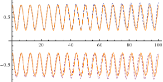
Figure 1: (Color online) Numerical result (dashed line) vs perturbative result (continuous line). In this figure, , , . The upper graph shows variation of as a function of time and the lower one shows variation of y as a function of time.
3 Quantum case
In order to quantize the classical Hamiltonian (13), we replace the classical variables by operators satisfying the commutation relations and the rest of the commutators are zero. We replace by and by and obtain the following expressions for the Hamiltonian and the conserved quantity in the quantum theory:
| (36) | |||||
| (37) |
The operators and commute and constitute two integrals of motion for the system which in turn implies that the system is integrable. Since and commute, it is always possible to chose a basis in which simultaneous eigen states of and may be constructed. An eigen function of the operator with continuous eigen values has the following form:
| (38) |
where is an arbitrary function of whose functional form is to be determined by demanding that is also an eigen function of the Hamiltonian H. In the limit of vanishing , the dependent part of is the wave function of a free particle with wave vector . This is consistent with the fact that in the same limit reduces to conjugate momentum operator up to an overall multiplication factor of two. Substituting (38) in the time independent Schrodinger equation,
| (39) |
we get the following equation:
| (40) |
This is a differential equation of only one variable . For vanishing , the centre of mass and the relative coordinates separate out in the Hamiltonian (13) and the Eq. (40) describes the motion of an isotonic oscillator. However, for , the centre of mass modes are coupled to the equation governed by . Similar situation arises in case for the system considered in Ref.[6] for which the Hamiltonian separates out into a free particle in centre of mass frame and a simple harmonic oscillator in the relative coordinate for . The term linear in in Eq. (40) for can always be absorbed by a shift of the relative coordinate for harmonic oscillator, but, not for isotonic oscillator. This poses difficulty in solving the Eq. (40).
The series solution method allows normalizable solution of (40) only for . Other nontrivial exact solutions are also not apparent. This is consistent with the fact that we obtain exact classical solutions when the value of the constant of motion is zero. Therefore, an obvious choice is to consider the exact normalizable solution corresponding to . In this case the Eq. (40) reduces to the following form:
| (41) |
This equation is invariant under the operation . Therefore the solutions may always be chosen to be either even or odd under parity transformation. The potential has a singularity at which breaks the space into two disjoint regions or and the wave function vanishes at . The ground state wave function and the corresponding energy of (41) are respectively given as
| (42) |
with and satisfying the relation . It is interesting to note that is real for the range . This indicates -symmetric phase transitions one at and other at . Outside this range the energy is complex and comes in complex conjugate pairs indicating a broken -symmetric region. Interestingly the classical and quantum -symmetric phase transitions occur at the same value of the parameter . In order to have the complete spectra we make the following substitution:
| (43) |
with which Eq. (41) reduces to the following form:
| (44) |
We demand a series solution of Eq. (44) having the form
| (45) |
The recursion relation for is given by
| (46) |
with , and is obtained from the normalization condition. Thus the series for contains only even powers of . For normalizable solutions, the series must be terminated and we get the following expression for the energy states
| (47) |
with being the ground state energy. If we now chose the positive sign of , then the ground state wave function is normalizable on the real line but the system becomes unbounded from below, i.e the system does not have a stable ground state. So we chose the negative sign for which makes the system bounded from below but in this case the normalization of the wave function becomes crucial and we discuss it below. If we write with , then first few polynomials may be written as
| (48) | |||
| (49) |
All the eigen states of of the form with , are the eigen states of belonging to the zero eigen value.
We now consider the normalization of the ground state wave function
| (50) |
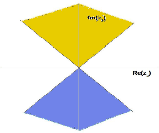
Clearly this wave function is not normalizable along the real line. We have to fix the Stoke wedges in the complex plane where the wave function is normalizable. The first part (-part) of the exponential vanishes in a pair of stoke wedges with opening angle and centered about the positive and negative imaginary axes in the complex -plane. The second part () of the exponential vanishes in the upper half of the complex -plane if the coefficient () of is negative and vanishes in the lower half of the complex plane if the coefficient () of is positive. Therefore vanishes in a single stoke wedges either with opening angle and centered about the positive imaginary axes in the complex -plane or with opening angle and centered about the negative imaginary axes in the complex -plane.
4 Conclusion
We have considered a two body rational Calogero model having balanced loss and gain. The Hamiltonian for the system is obtained which is found to be symmetric. This system admits two integral of motions in involution. This system is integrable both classically and quantum mechanically. In particular, the classical Eqs. of motion for the system are solved exactly for the particular ranges of the parameters. We obtained exact, stable classical solutions. We also quantized this classical model. The quantized system yields bound state solutions for exactly the same range of the parameters for which the classical solutions are stable. The normalization of the wave functions in the proper Stoke wedges are discussed. Further, the Calogero model with balanced loss and gain is studied classically, when the pair-wise harmonic interaction term is replaced by a common confining harmonic potential. This system may be considered as the Sutherland model in the presence of balanced loss and gain. The integrability of this system is obscure. In the classical level, the stability analysis is carried out and perturbative solutions are obtained. Finally, this perturbative results are compared with the numerical results. In our study we only focus on two-body problem. The question of many-body generalization of coupled oscillators system having balanced loss and gain and are interacting via Calogero-Sutherland type of potential will be very much interesting.
5 Acknowledgements
This work is partly supported by a grant(DST Ref. No. SR/S2/HEP-24/2012) from Science & Engineering Research Board(SERB), Department of Science & Technology(DST), Govt. of India. DS acknowledges a research fellowship from CSIR.
References
- [1] H. Bateman, Phys. Rev. 38, 815 (1931).
- [2] H. Dekker, Phys. Rep. 80, 1 (1981).
- [3] E. Celeghini, M. Rasetti, and G. Vitiello, Ann. Phys. (N.Y.) 215, 156 (1992).
- [4] R. Banerjee and P. Mukherjee, J. Phys. A 35, 5591 (2002).
- [5] D. Chruscinski and J. Jurkowski, Ann. Phys. (N.Y.) 321, 854 (2006).
- [6] C. M. Bender, M. Gianfreda, S. K. Ozdemir, B. Peng and L. Yang, Phys. Rev. A 88, 062111 (2013).
- [7] R. Banerjee and P. Mukherjee, Mod.Phys.Lett. A30, 1550193 (2015).
- [8] B. Peng, S. K. Ozdemir, F. Lei, F. Monifi, M. Gianfreda, G. L. Long, S. Fan, F. Nori, C. M. Bender, and L. Yang, Nature Physics 10, 394 (2014).
- [9] J. Schindler, A. Li, M. C. Zheng, F. M. Ellis, and T. Kottos, Phys. Rev. A 84, 040101(R) (2011).
- [10] C. M. Bender, M. Gianfreda, and S. P. Klevansky Phys. Rev. A 90, 022114 (2014).
- [11] J. Cuevas, P. G. Kevrekidis, A. Saxena and A. Khare, Phys. Rev. A 88, 032108 (2013).
- [12] I. V. Barashenkov and M. Gianfreda, J. Phys. A: Math. Theor. 47, 282001(2014).
- [13] F. Calogero, Jour. Math. Phys. 10, 2191 (1969).
- [14] F. Calogero, Jour. Math. Phys. 10, 2197 (1969).
- [15] F. Calogero, Jour. Math. Phys. 12, 419 (1971).
- [16] B. Sutherland, J. Math. Phys.(N.Y.)12, 246 (1971).
- [17] B. Sutherland, J. Math. Phys. 12, 251 (1971).
- [18] B. Sutherland, Phys.Rev. A 4, 2019 (1971).
- [19] M. A. Olshanetsky and A. M. Perelomov, Phys. Rep. 71, 314 (1981).
- [20] M. A. Olshanetsky and A. M. Perelomov, Phys. Rep. 94, 6(1983).
- [21] A. P. Polychronakos, Phys. Rev. Lett. 69, 703 (1992).
- [22] P. K. Ghosh, J. Phys. A: Math. Theor. 45, 183001 (2012).
- [23] M. V. N. Murthy and R. Shankar, Phys. Rev. Lett. 73, 3331(1994).
- [24] B. D. Simons, P. A. Lee and B. Altshuler, Phys. Rev. Lett. 72, 64 (1994).
- [25] S. Jain, Mod. Phys. Lett. A 11, 1201 (1996).
- [26] F. D. M. Haldane, Phys. Rev. Lett. 60, 635 (1988).
- [27] B. S. Shastry, Phys. Rev. Lett. 60, 639 (1988).
- [28] K. Hikami and M. Wadati, Phys. Rev. Lett. 73, 1191 (1994).
- [29] H. Ujino and M. Wadati, J. Phys. Soc. Jap. 63, 3585 (1994).
- [30] B. Basu-Mallick, P. K. Ghosh and Kumar S. Gupta, Phys. Lett. A 311, 87 (2003), hep-th/0208132.
- [31] B. Basu-Mallick, P. K. Ghosh and Kumar S. Gupta, Nucl. Phys. B 659, 437 (2003), hep-th/0207040.
- [32] B. Basu-Mallick, P. K. Ghosh and Kumar S. Gupta, Pramana-J. Phys. 62, 691 (2004).
- [33] B. Basu-Mallick and Kumar S. Gupta, Phys. Lett. A 292, 36 (2001), hep-th/0109022.
- [34] V. Bardek, J. Feinberg, S. Meljanac, JHEP 08, 018 (2010).
- [35] V. Bardek, J. Feinberg, S. Meljanac, Annals of Physics 325, 691 (2010).