Machine Learning Techniques for Mortality Modeling

Abstract

Various stochastic models have been proposed to estimate mortality rates. In this paper we illustrate how machine learning techniques allow us to analyze the quality of such mortality models. In addition, we present how these techniques can be used for differentiating the different causes of death in mortality modeling.

Keywords: mortality modeling, cause-of-death mortality, machine learning, boosting, regression.

1 Introduction

Mortality modeling is crucial in economy, demography and in life and social insurance, because mortality rates determine insurance liabilities, prices of insurance products, and social benefit schemes. As such, many different stochastic mortality models to estimate and forecast these rates have been proposed, starting from the Lee-Carter [5] model. For a broad overview and comparison of existing models we refer to [3]. In this article we revisit two of these models and study their calibration to Swiss mortality data. We illustrate how machine learning techniques allow us to study the adequacy of the estimated mortality rates. By applying a regression tree boosting machine we analyze how the modeling should be improved based on feature components of an individual, such as its age or its birth cohort. This (non-parametric) regression approach then allows us to detect the weaknesses of different mortality models.

In a second part of this work we investigate cause-of-death mortality. Given a death of an individual with a specific feature, we study the conditional probability of its cause. Based on Swiss mortality data we illustrate how regression tree algorithms can be applied to estimate these conditional probabilities in a Poisson model framework. The presented technique provides a simple way to detect patterns in these probabilities over time. For a parametric modeling approach and existing literature on cause-of-death mortality we refer to [1, 4] and references therein.

Organization of the paper. In the next section we introduce the notation and state the model assumptions. In Section 3 we analyze two standard models, the Lee-Carter [5] model and the Renshaw-Haberman [7] model, and we explain how machine learning techniques can be applied to investigate the adequacy of these models for a given dataset. Note that we do not consider the most sophisticated models here, but our goal is to study well-known standard models and to indicate how their strengths and weaknesses can be detected with machine learning. In Section 4 we refine these models to the analysis of cause-of-death mortality.

2 Model assumptions

In mortality modeling each individual person is identified by its gender, its age, and the calendar year (also called period) in which the person is considered. As such, each individual person is assigned to a feature ${\bm{x}}=(g,a,t)\in{\mathcal{X}}={\mathcal{G}}\times{\mathcal{A}}\times{\mathcal{T}}$, with feature components

$${\mathcal{G}}=\{\text{female, male}\},\quad{\mathcal{A}}=\{0,\ldots,\omega\},\quad\text{ and }\quad{\mathcal{T}}=\{t_{\text{min}},\ldots,t_{\text{max}}\}.$$ (2.1)

Here, $a\in{\mathcal{A}}$ represents the age in years of the person, $\omega\in{\mathbb{N}}$ denotes the maximal possible age the person can reach. The component ${\mathcal{T}}\subset{\mathbb{N}}_{0}$ describes the calendar years considered. This feature space ${\mathcal{X}}={\mathcal{G}}\times{\mathcal{A}}\times{\mathcal{T}}$ could be extended by further feature components such as the income or marital status of a person, however, for our study we do not have additional individual information.

For a given feature ${\bm{x}}=(g,a,t)\in{\mathcal{X}}$ we denote the (deterministic) exposure by $E_{{\bm{x}}}\geq 1$ and the corresponding (random) number of deaths by $D_{{\bm{x}}}\geq 0$. That is, for a given feature ${\bm{x}}=(g,a,t)\in{\mathcal{X}}$ we have $E_{\bm{x}}$ people with feature ${\bm{x}}$ alive at the beginning of the period $(t,t+1]$, and during this period $D_{\bm{x}}$ of these people die. Two assumptions commonly made in the literature are that $D_{\bm{x}}$ are independent, for different ${\bm{x}}\in{\mathcal{X}}$, and each $D_{\bm{x}}$ has a Poisson distribution with a parameter proportional to $E_{\bm{x}}$. This also assumes that the force of mortality stays constant over each period $(t,t+1]$. In this spirit, we consider the following model assumptions.

Model Assumptions 2.1.

Assume that the mortality rates are given by the regression function $q:{\mathcal{X}}\to[0,1]$, ${\bm{x}}\mapsto q({\bm{x}})$. The numbers of deaths satisfy the following properties:

• $(D_{\bm{x}})_{{\bm{x}}\in{\mathcal{X}}}$ are independent in ${\bm{x}}\in{\mathcal{X}}$.

• $D_{\bm{x}}~{}\sim~{}\text{Pois}(q({\bm{x}})E_{\bm{x}})$ for all ${\bm{x}}\in{\mathcal{X}}$;

The main difficulty is to appropriately estimate the mortality rates $q:{\mathcal{X}}\to[0,1]$ from historical data of a given population. In particular, we would like to infer $q(\cdot)$ from observations. Several models have been developed in the literature to address this problem. In the next section we consider two standard models and we explain how machine learning techniques can be applied to back-test these two models.

3 Boosting mortality rates

We investigate two different classical models for estimating mortality rates: the Lee-Carter [5] model and the Renshaw-Haberman [7] model. By applying machine learning techniques we analyze the weaknesses of these models. Note that this illustration has mainly pedagogical value. First, the Lee-Carter model is a comparably simple model that has been improved in many directions in various research studies. Second, one of these improvements is the Renshaw-Haberman model that we will compare to the Lee-Carter model.

The following analysis is based on historical Swiss mortality data provided by the Human Mortality Database, see www.mortality.org. The data we consider includes the exposures $(E_{\bm{x}})_{{\bm{x}}\in{\mathcal{X}}}$ and the numbers of deaths $(D_{\bm{x}})_{{\bm{x}}\in{\mathcal{X}}}$ for the feature space ${\mathcal{X}}={\mathcal{G}}\times{\mathcal{A}}\times{\mathcal{T}}$ with feature components

$${\mathcal{G}}=\{\text{female, male}\},\quad{\mathcal{A}}=\{0,1,\ldots,97\},\quad\text{and}\quad{\mathcal{T}}=\{1876,1877,\ldots,2014\}.$$

Here, maximal age $a=97$ corresponds to ages of at least $97$, and the set ${\mathcal{T}}$ consists of $139$ years of observations. This results in $2\cdot 98\cdot 139=\,$27,244 data points corresponding to 7,867,978 deaths within those $139$ years of observations.

3.1 Back-testing the Lee-Carter model

We first consider the classical Lee-Carter [5] model and we apply regression tree boosting to detect its weaknesses. The Lee-Carter model is a comparably simple model in which the mortality rates are assumed to be of the form

$$q^{\text{LC}}({\bm{x}})~{}=~{}\exp\left\{\beta^{0,g}_{a}+\beta^{1,g}_{a}\kappa^{g}_{t}\right\},\qquad\text{for ${\bm{x}}=(g,a,t)\in{\mathcal{X}}$,}$$

with the identifiability constraints $\sum_{a}\beta^{1,g}_{a}=1$ and $\sum_{t}\kappa^{g}_{t}=0$ for each $g\in{\mathcal{G}}$. For fixed gender $g\in{\mathcal{G}}$ we fit the parameters $\beta^{0,g}_{a}$, $\beta^{1,g}_{a}$, and $\kappa^{g}_{t}$ to the Swiss mortality data using the ‘StMoMo’ R-package, see [11], as follows

>  LC <- fit(lc(link="log"),  Dxt = deaths,  Ext = exposures)
>  q.LC <- fitted(LC, type = "rates") 3.1

The exposures $(E_{{\bm{x}}})_{{\bm{x}}\in{\mathcal{X}}}$ and the numbers of deaths $(D_{{\bm{x}}})_{{\bm{x}}\in{\mathcal{X}}}$ are the input data, and we apply the above command to each gender $g\in{\mathcal{G}}$ separately. q.LC then provides the Lee-Carter mortality rates $(q^{\text{LC}}({\bm{x}}))_{{\bm{x}}\in{\mathcal{X}}}$ fitted to the Swiss data. These rates are presented in Figure 1 by dashed lines, and compared to the crude (observed) mortality rates $D_{\bm{x}}/E_{\bm{x}}$ illustrated by dots in Figure 1. We aim at back-testing these fitted mortality rates by using machine learning techniques. For this, we initialize Model Assumptions 2.1 with the rates $q({\bm{x}})=q^{\text{LC}}({\bm{x}})$ obtained from the Lee-Carter fit (3.1), i.e., we consider for ${\bm{x}}\in{\mathcal{X}}$,

$$D_{\bm{x}}~{}\sim~{}\text{Pois}(\mu({\bm{x}})d_{\bm{x}}),\qquad\text{with $\mu({\bm{x}})\equiv 1$ and $d_{\bm{x}}=q^{\text{LC}}({\bm{x}})E_{\bm{x}}$}.$$ (3.2)

Observe that $d_{\bm{x}}$ describes the expected number of deaths according to the Lee-Carter fit. To back-test this model we analyze whether the constant factor $\mu({\bm{x}})\equiv 1$ is an appropriate choice for the Swiss data considered. For instance, for given feature ${\bm{x}}\in{\mathcal{X}}$ this factor $\mu({\bm{x}})$ should be increased if the Lee-Carter mortality rate $q^{\text{LC}}({\bm{x}})$ underestimates the crude rate $D_{\bm{x}}/E_{\bm{x}}$. As such, our aim is to calibrate the factor $\mu({\bm{x}})$ in (3.2) based on the chosen features ${\bm{x}}\in{\mathcal{X}}$.

To do so, we apply one step of the Poisson Regression Tree Boosting Machine to the working data $(D_{\bm{x}},\,{\bm{x}},\,d_{\bm{x}})_{{\bm{x}}\in{\mathcal{X}}}$, see [2] and Section 6.4 in [13]. This standardized binary split (SBS) tree growing algorithm selects at each iteration step a feature component (gender, age or calendar year) and splits the feature space ${\mathcal{X}}$ in a rectangular way with respect to this chosen feature component. The explicit choice of each split is based on an optimal improvement of a given loss function that results from that split. The algorithm then provides an SBS Poisson regression tree estimator $\hat{\mu}({\bm{x}})$, ${\bm{x}}\in{\mathcal{X}}$, that is calibrated on each rectangular subset of ${\mathcal{X}}$ obtained from these splits. That is, we obtain $\hat{\mu}(\cdot)$ as a calibration of $\mu(\cdot)$ using this non-parametric regression approach; we refer to [13] for further details on this regression tree boosting.

Observe that the SBS tree growing algorithm calibrates $\mu(\cdot)$ by generating only rectangular splits of the feature space ${\mathcal{X}}$. However, we would like to calibrate the factor $\mu(\cdot)$ also with respect to birth cohorts, which requires diagonal splits of the feature space. For this reason we extend the feature space ${\mathcal{X}}$ to the feature space $\bar{\mathcal{X}}=\{(g,a,t,c=t-a)\mid g\in{\mathcal{G}},\,a\in{\mathcal{A}},\,t\in{\mathcal{T}}\}$, where $c=t-a$ provides the cohort of feature ${\bm{x}}=(g,a,t)\in{\mathcal{X}}$. Observe that there is a one-to-one correspondence between ${\mathcal{X}}$ and $\bar{\mathcal{X}}$, but this extension is necessary to allow for sufficient degrees of freedom in SBSs. From this we see that a smart model design includes a thoughtful choice of the feature space, allowing for the desired interactions and dependencies.

We apply the SBS tree growing algorithm to calibrate $\mu(\cdot)$ in (3.2) with respect to the (extended) feature space $\bar{\mathcal{X}}$. This is obtained in R using the ‘rpart’ package, see [10], and the input

>  tree <- rpart(cbind(volume,deaths) $\sim$ gender + age + year + cohort,
                                                                      data = data, method = "poisson",
                                                                      cp = 2e-3)

>  mu <- predict(tree) 3.3

Here, the data contains for each feature ${\bm{x}}=(g,a,t)\in{\mathcal{X}}$ the volume $d_{\bm{x}}$ and the number of deaths $D_{\bm{x}}$, and we optimize subject to gender $g$, age $a$, year $t$, and cohort $c=t-a$. The cost-complexity parameter cp allows us to control the number of iteration steps performed by the regression tree algorithm, for more details on this control parameter we refer to Section 5.2 of [13]. The regression tree estimator $\hat{\mu}(\cdot)$ is then given by mu. This estimator allows us to define the regression tree improved mortality rates

$$q^{\text{tree}}({\bm{x}})~{}=~{}\hat{\mu}({\bm{x}})q^{\text{LC}}({\bm{x}}),\qquad\text{ for ${\bm{x}}\in{\mathcal{X}}$.}$$ (3.4)

These mortality rates are illustrated in Figure 1 by lines and compared to the Lee-Carter fit $q^{\text{LC}}({\bm{x}})$ presented by dashed lines.

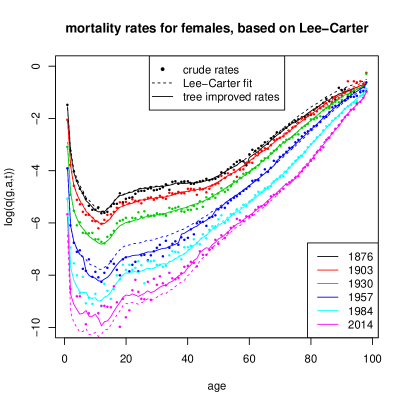
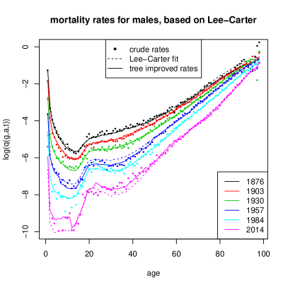
Figure 1: Logarithms of mortality rates for (lhs) females and (rhs) males, for different ages and calendar years. The dots illustrate the crude mortality rates of the Swiss mortality data, the dashed lines the Lee-Carter fit, and the solid lines illustrate the tree improved estimates given by (3.4).

In order to analyze the improvements in the initialized mortality rates $q^{\text{LC}}({\bm{x}})$ obtained by the tree growing algorithm, we consider the relative changes

$$\Delta q^{\text{LC}}({\bm{x}})~{}=~{}\frac{q^{\text{tree}}({\bm{x}})-q^{\text{LC}}({\bm{x}})}{q^{\text{LC}}({\bm{x}})}~{}=~{}\hat{\mu}({\bm{x}})-1,\qquad\text{ for ${\bm{x}}\in{\mathcal{X}}$.}$$

These relative changes are presented in the first row of Figure 2.

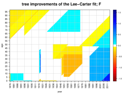
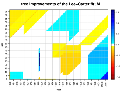
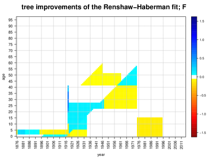
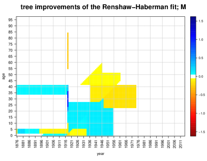
Figure 2: Changes in mortality rates $\Delta q^{\text{LC}}({\bm{x}})$ (first row) and $\Delta q^{\text{RH}}({\bm{x}})$ (second row), respectively, obtained by the boosting step of the tree growing algorithm. The first column shows the changes for females, the second one for males. Small changes in the range $[-5\%,5\%]$ are illustrated in white color.

We observe substantial changes in the calibrated mortality rates for many parts of the feature space ${\mathcal{X}}$. For instance, we see that the algorithm remarkably increases the Lee-Carter mortality rates for the calendar year $t=1918$, when the Spanish flu had its spike. This is not surprising, since the Lee-Carter model does not appropriately capture the impacts of such special events, see also the discussions in [5, 6]. A main observation is that the algorithm performs many splits with respect to birth cohorts (diagonals in Figure 2), many of them are performed in the very first iteration steps. This means that these splits particularly reduce the value of the loss function considered by the algorithm and lead to a substantial improvement in the fit. As an example, the algorithm improves the initialized mortality rates $q^{LC}({\bm{x}})$ for features ${\bm{x}}$ with birth cohort $c=t-a=1816$, which is called “the year without a summer”; we refer to [9] for historical information. Again, this is not surprising, since the Lee-Carter framework does not account for such cohort effects, see also [6]. We conclude that these cohort effects motivate us to perform a similar analysis on the Renshaw-Haberman model which aims at addressing this drawback of the Lee-Carter model.

3.2 Back-testing the Renshaw-Haberman model

In this section we consider the Renshaw-Haberman [7] model, which is a cohort-based extension to the classical Lee-Carter model discussed in the previous section. In the Renshaw-Haberman model the mortality rates are assumed to be of the form

$$q^{\text{RH}}({\bm{x}})~{}=~{}\exp\left\{\beta^{0,g}_{a}+\beta^{1,g}_{a}\kappa^{g}_{t}+\beta^{2,g}_{a}\gamma^{g}_{t-a}\right\},\qquad\text{for ${\bm{x}}=(g,a,t)\in{\mathcal{X}}$,}$$

with the identifiability constraints

$$\sum_{a}\beta^{1,g}_{a}=\sum_{a}\beta^{2,g}_{a}=1\qquad\text{and}\qquad\sum_{a,t}\gamma^{g}_{t-a}=\sum_{t}\kappa^{g}_{t}=0,\qquad\text{for each $g\in{\mathcal{G}}$. }$$

Observe that, compared to the Lee-Carter framework, we have additional terms $\beta^{2,g}_{a}\gamma^{g}_{t-a}$ that allow the model to capture cohort effects. We fit the Renshaw-Haberman model to the Swiss mortality data. This is achieved in R similarly to the Lee-Carter model using the command rh() instead of lc() in input (3.1). From this we obtain the fitted mortality rates $q^{\text{RH}}({\bm{x}})$, ${\bm{x}}\in{\mathcal{X}}$, and we initialize Model Assumptions 2.1 with these rates $q({\bm{x}})=q^{\text{RH}}({\bm{x}})$. Then, we apply the same regression tree boosting machine as explained in Section 3.1 to obtain regression tree improved mortality rates $q^{\text{tree}}({\bm{x}})$ as well as the corresponding relative changes $\Delta q^{\text{RH}}({\bm{x}})=q^{\text{tree}}({\bm{x}})/q^{\text{RH}}({\bm{x}})-1$, ${\bm{x}}\in{\mathcal{X}}$.

The second row of Figure 2 illustrates these relative changes $\Delta q^{\text{RH}}({\bm{x}})$ in the mortality rates. We first compare these changes to the changes $\Delta q^{\text{LH}}({\bm{x}})$ obtained in Section 3.1 based on the Lee-Carter model, see first row of Figure 2. We observe that for the Renshaw-Haberman fit the regression tree algorithm proposes less adjustments than for the Lee-Carter fit. In particular, for ages above $60$ there are no changes $\Delta q^{\text{RH}}({\bm{x}})$ outside the range $[-5\%,5\%]$, except for the calendar year $t=1918$. On the one hand, this illustrates that for these ages the Renshaw-Haberman fit is quite appropriate and better than the Lee-Carter fit. On the other hand, year $t=1918$ indicates that the Renshaw-Haberman model may not fully capture special events such as epidemics, see also the split for birth cohort $c=t-a=1917$ in Figure 2. This is mainly explained by the fact that special events are too heavy-tailed for this model choice. Moreover, not surprisingly, the algorithm performs only a few splits with respect to birth cohorts in the Renshaw-Haberman model; indeed it captures cohort effects more appropriately compared to the Lee-Carter model. Finally, compared to the Lee-Carter model, we observe that the Renshaw-Haberman framework provides better mortality fits for recent calendar years between $t=1986$ and $t=2014$.

4 Boosting cause-of-death mortality

In this section we discuss cause-of-death mortality under the Poisson framework of Model Assumptions 2.1. Given a death with specific feature ${\bm{x}}\in{\mathcal{X}}$, we investigate the conditional probability of its cause. We illustrate how these probabilities can be estimated from real data by applying Poisson regression tree boosting similarly as introduced in Section 3. This allows us to detect patterns in these probabilities over time. We first introduce the setup and then apply the boosting machine to Swiss mortality data.

4.1 Cause-of-death mortality framework

Consider the feature space ${\mathcal{X}}={\mathcal{G}}\times{\mathcal{A}}\times{\mathcal{T}}$ with components given by (2.1). Again, one could consider further feature components such as the socio-economic status of a person. We fix Model Assumptions 2.1 with given (estimated) mortality rates $q({\bm{x}})$, ${\bm{x}}\in{\mathcal{X}}$, and we consider the set ${\mathcal{K}}=\{1,\ldots,K\}$ that describes $K\in{\mathbb{N}}$ different possible causes of death. Conditionally given a death with feature ${\bm{x}}\in{\mathcal{X}}$, we denote by $\theta(k|{\bm{x}})\in[0,1]$ the conditional probability that the corresponding cause is $k\in{\mathcal{K}}$, and we denote by $D_{{\bm{x}},k}\geq 0$ the number of such deaths. Since ${\mathcal{K}}$ provides a partition, we get $\sum_{k}D_{{\bm{x}},k}=D_{{\bm{x}}}$ and $\sum_{k}\theta(k|{\bm{x}})=1$ for all ${\bm{x}}\in{\mathcal{X}}$. Furthermore, under Model Assumptions 2.1 we obtain

$$D_{{\bm{x}},k}~{}\sim~{}\text{Pois}\left(\theta(k|{\bm{x}})q({\bm{x}})E_{{\bm{x}}}\right),$$ (4.1)

and $(D_{{\bm{x}},k})_{{\bm{x}},k}$ are independent, see Theorem 2.14 in [12]. Note that (4.1) is subject to $\theta(k|{\bm{x}})>0$, otherwise we set $D_{{\bm{x}},k}=0$, ${\mathbb{P}}$-a.s. As an initial model (prior choice) we assume that the probabilities $\theta(k|{\bm{x}})$ are independent of any features ${\bm{x}}\in{\mathcal{X}}$ and of any cause $k\in{\mathcal{K}}$, and we simply set

$$\theta(k|{\bm{x}})~{}=~{}\theta_{K}~{}=~{}\frac{1}{K},\qquad\text{for $k\in{\mathcal{K}}$ and ${\bm{x}}\in{\mathcal{X}}$.}$$

Alternative initializations, such as observed relative frequencies, could be chosen as well. This provides the input (starting value) for the subsequent boosting machine to calibrate the conditional probabilities $\theta(\cdot|{\bm{x}})$. Using (4.1) we write

$$D_{{\bm{x}},k}~{}\sim~{}\text{Pois}(\mu({\bm{x}},k)d_{{\bm{x}},k})\qquad\text{with $\mu({\bm{x}},k)\equiv 1$ and $d_{{\bm{x}},k}=\theta(k|{\bm{x}})q({\bm{x}})E_{{\bm{x}}}$},$$

for ${\bm{x}}\in{\mathcal{X}}$ and $k\in{\mathcal{K}}$. According to our initial model assumptions, $d_{{\bm{x}},k}$ denotes the expected number of deaths with feature ${\bm{x}}\in{\mathcal{X}}$ and with cause of death being $k\in{\mathcal{K}}$. Our aim is to calibrate the factor $\mu(\cdot):{\mathcal{X}}\times{\mathcal{K}}\to{\mathbb{R}}_{+}$ by a non-parametric regression approach in complete analogy to Section 3.1.

For this we apply the SBS tree growing algorithm to the working data $(D_{{\bm{x}},k},\,({\bm{x}},k),\,d_{{\bm{x}}.k})_{{\bm{x}},k}$ based on the extended feature space $\{(g,a,t,c=t-a,k)\mid g\in{\mathcal{G}},\,a\in{\mathcal{A}},\,t\in{\mathcal{T}},\,k\in{\mathcal{K}}\}$. That is, we calibrate the factor $\mu(\cdot)$ with respect to the feature components gender, age, calendar year, birth cohort and cause of death by using the R-command similar to the one in (3.1). This provides us a tree based estimator $\hat{\mu}({\bm{x}},k)$ of $\mu({\bm{x}},k)$, and allows us to define the regression tree estimated probabilities

$$\theta^{\text{tree}}(k|{\bm{x}})~{}=~{}\hat{\mu}({\bm{x}},k)\theta(k|{\bm{x}}),\qquad\text{for $k\in{\mathcal{K}}$ and ${\bm{x}}\in{\mathcal{X}}$.}$$ (4.2)

Here, we interpret $\hat{\mu}({\bm{x}},k)$ as a refinement of the initial conditional probability $\theta(k|{\bm{x}})=\theta_{K}=1/K$. Instead, $\hat{\mu}({\bm{x}},k)$ could also be interpreted as an improvement of the unconditional probability $\theta(k|{\bm{x}})q({\bm{x}})$. However, in our context, we consider the initialized mortality rates $q({\bm{x}})$ as fixed.

4.2 Boosting Swiss cause-of-death mortality data

We apply regression tree boosting as explained in the previous section to Swiss cause-of-death mortality data provided by the Swiss Federal Statistical Office and by the Human Mortality Database, see also Section 3. This data includes the exposures $(E_{{\bm{x}}})_{{\bm{x}}}$ and the numbers of deaths $(D_{{\bm{x}},k})_{{\bm{x}},k}$ for the feature space ${\mathcal{X}}={\mathcal{G}}\times{\mathcal{I}}\times{\mathcal{T}}$ with feature components

$${\mathcal{G}}=\{\text{female, male}\},\quad{\mathcal{I}}=\{1,2,\ldots,6\},\quad\text{and}\quad{\mathcal{T}}=\{1990,1991,\ldots,2014\},$$

and for ${\mathcal{K}}=\{1,\ldots,12\}$ describing $12$ different causes of death, see below. Because our data on cause-of-death mortality only contains limited information about the age of a person, we have replaced the feature component ${\mathcal{A}}$ by the feature component ${\mathcal{I}}$ that represents six disjoint age buckets. Age group $i=1$ corresponds to age $0$, $i=2$ to ages $1-14$, $i=3$ to ages $15-44$, $i=4$ to ages $45-64$, $i=5$ to ages $65-84$, and $i=6$ corresponds to ages of at least $85$. The set ${\mathcal{K}}$ represents the following $K=12$ different possible causes of death:

1) infectious diseases	5) circulatory system	9) congenital malformation
2) malignant tumors	6) respiratory organs	10) perinatal causes
3) diabetes mellitus	7) alcoholic liver cirrhosis	11) accidents and violent impacts
4) dementia	8) urinary organs	12) others/unknown

The data $D_{{\bm{x}},k}$ for cause $k=4$ (dementia) is not available for the first five years of observations $t\in\{1990,\ldots,1994\}$. However, the rpart() command of the ‘rpart’ package is able to cope with such missing data, see [10] for details.

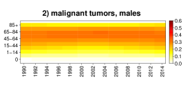
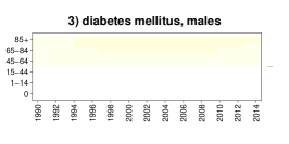
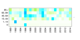
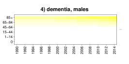
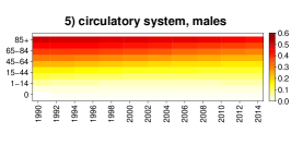
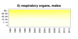
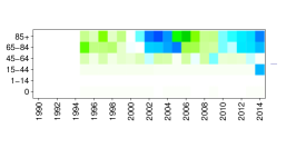
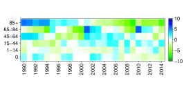
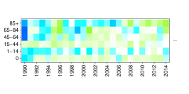
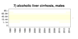
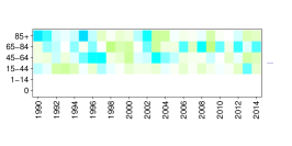
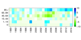
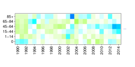
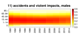
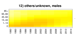
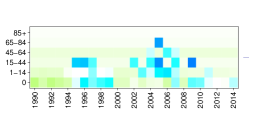
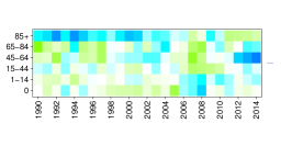
Figure 6: The odd rows illustrate the regression tree estimated probabilities $\theta^{\text{tree}}(k|{\bm{x}})$ for males. These plots all have the same scale given in the middle plot in each odd row. The even rows show the corresponding Pearson’s residuals given by (4.3). These plots all have the same scale given in the middle plot in each even row.

We initialize Model Assumptions 2.1 with the regression tree improved mortality rates $q({\bm{x}})=q^{\text{tree}}({\bm{x}})$, ${\bm{x}}\in{\mathcal{X}}$, obtained in Section 3.2 based on the Renshaw-Haberman fit. Observe that this needs some care because we work here on a feature space that is different to the one in Section 3, see Remark 4.1, below. Then, we apply the SBS tree growing algorithm based to the feature space ${\mathcal{X}}\times{\mathcal{K}}$; note that here we do not calibrate $\hat{\mu}$ with respect to birth cohorts. This provides us with the regression tree estimated conditional probabilities $\theta^{\text{tree}}(k|{\bm{x}})$ for $k\in{\mathcal{K}}$ and ${\bm{x}}\in{\mathcal{X}}$, according to (4.2). The resulting probabilities for females and the causes of death $k=2$ (malignant tumors) and $k=5$ (circulatory system), respectively, are presented in the first row of Figure 3; the remaining probabilities are summarized in Appendix A, in Figure 5 for females and in Figure 6 for males. We have applied a polynomial smoothing model to these plots in order to present the tree estimated probabilities in a more accessible way. The second row of Figure 3 shows the corresponding Pearson’s residuals given by

$$\delta^{\text{tree}}_{{\bm{x}}|k}~{}=~{}\frac{D_{{\bm{x}},k}-\theta^{\text{tree}}(k|{\bm{x}})D_{\bm{x}}}{\sqrt{\theta^{\text{tree}}(k|{\bm{x}})D_{\bm{x}}}},\qquad\text{for ${\bm{x}}\in{\mathcal{X}}$ and $k\in{\mathcal{K}}$,}$$ (4.3)

where we set $\delta^{\text{tree}}_{{\bm{x}}|k}=0$ if the denominator equals $0$ or if the data on $D_{{\bm{x}},k}$ is missing. We observe that the regression tree boosting machine has suitably estimated the probabilities $\theta(k|{\bm{x}})$, there are no structures visible in the residual plots. However, note that the interpretation of these estimates $\theta^{\text{tree}}(k|{\bm{x}})$ needs some care. For instance, the classification of certain causes of death may have changed over time, see also the discussion in [8].

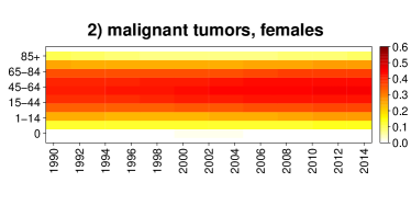
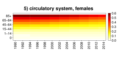
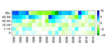
Figure 3: The first row illustrates the regression tree estimated probabilities $\theta^{\text{tree}}(k|{\bm{x}})$ for females and for the causes of death $k\in\{2,5\}$. The second row shows the corresponding Pearson’s residuals defined in (4.3).

Figure 4 shows the evolution of the different cause-of-death probabilities over time for males aged between $45$ and $64$; the probabilities for the remaining age classes are presented in Appendix A, in Figure 7 for females and in Figure 8 for males.

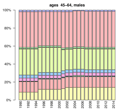
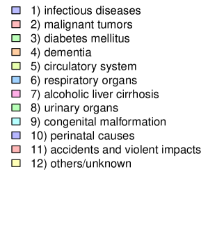
Figure 4: Regression tree estimated probabilities $\theta^{\text{tree}}(k|{\bm{x}})$ for the $12$ different causes of death considered, conditionally for males aged between $45$ and $64$.

Remark 4.1.

Consider the feature space ${\mathcal{X}}={\mathcal{G}}\times{\mathcal{A}}\times{\mathcal{T}}$ with feature components as in (2.1), and consider Model Assumptions 2.1 with given mortality rates $q({\bm{x}})$, ${\bm{x}}\in{\mathcal{X}}$. Additionally, consider the condensed feature space $\tilde{\mathcal{X}}={\mathcal{G}}\times{\mathcal{I}}\times{\mathcal{T}}$, with ${\mathcal{I}}=\{1,\ldots,I\}$ representing $I\geq 1$ disjoint and non-empty age buckets ${\mathcal{A}}_{1},\ldots,{\mathcal{A}}_{I}\subset{\mathcal{A}}$ that form a partition of ${\mathcal{A}}$. In the following we briefly sketch how to construct mortality rates $\tilde{q}(\tilde{\bm{x}})$, $\tilde{\bm{x}}\in\tilde{\mathcal{X}}$, from $q(\cdot)$ in a way that is consistent with Model Assumptions 2.1 for the condensed feature space $\tilde{\mathcal{X}}$.

For ${\bm{x}}=(g,a,t)\in{\mathcal{X}}$ and $\tilde{\bm{x}}=(\tilde{g},i,\tilde{t})\in\tilde{\mathcal{X}}$ we write ${\bm{x}}\sim\tilde{\bm{x}}$ if $g=\tilde{g}$, $a\in{\mathcal{A}}_{i}$ and $t=\tilde{t}$. Consider the mortality rates given by the regression function $\tilde{q}:\tilde{\mathcal{X}}\to[0,1]$ with

$$\tilde{q}(\tilde{\bm{x}})~{}=~{}\frac{1}{E_{\tilde{\bm{x}}}}\sum_{{\bm{x}}\sim\tilde{\bm{x}}}E_{{\bm{x}}}\,q({\bm{x}}),\qquad\tilde{\bm{x}}\in\tilde{\mathcal{X}},$$ (4.4)

with $E_{\tilde{\bm{x}}}=\sum_{{\bm{x}}\sim\tilde{\bm{x}}}E_{{\bm{x}}}$ denoting the total exposure with condensed feature $\tilde{\bm{x}}\in\tilde{\mathcal{X}}$. Denote by $D_{\tilde{\bm{x}}}=\sum_{{\bm{x}}\sim\tilde{\bm{x}}}D_{{\bm{x}}}$ the total number of deaths with condensed feature $\tilde{\bm{x}}\in\tilde{\mathcal{X}}$. By Model Assumptions 2.1 we obtain

$$D_{\tilde{\bm{x}}}~{}\sim~{}\text{Pois}\left(\sum_{{\bm{x}}\sim\tilde{\bm{x}}}q({\bm{x}})E_{{\bm{x}}}\right)~{}\overset{(\text{d})}{=}~{}\text{Pois}(\tilde{q}(\tilde{\bm{x}})E_{\tilde{\bm{x}}}),$$

and these random variables are independent in $\tilde{\bm{x}}\in\tilde{\mathcal{X}}$, see Theorem 2.12 in [12]. That is, the mortality rates $\tilde{q}(\cdot)$ given by (4.4) are defined in a way that is consistent with Model Assumptions 2.1 for the condensed feature space $\tilde{\mathcal{X}}$. In particular, our model assumptions are closed towards aggregations that give more coarse partitions.

5 Conclusions

In a first analysis we have illustrated how machine learning techniques, in particular the regression tree boosting machine, can be used in order to back-test parametric mortality models. These techniques allow us to detect the weaknesses of such models based on real data. Moreover, regression tree boosting can further be applied to improve the fits of such models with respect to feature components that are not captured by these models. Typical examples are education, income or marital status of a person.

In the second part we have investigated cause-of-death mortality under a Poisson model framework. We have presented how regression tree boosting can be applied to estimate cause-of-death mortality rates from real data. This technique provides a simple way to detect patterns in these probabilities over time.

Appendix A Figures on Swiss cause-of-death mortality

 

 

 

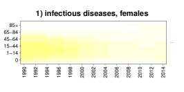
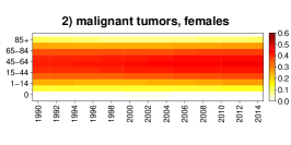
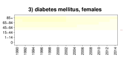
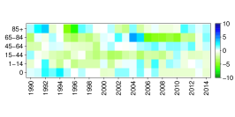
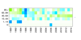
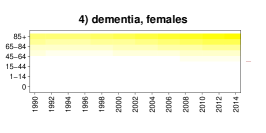
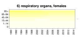
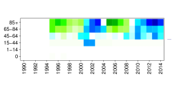
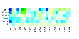
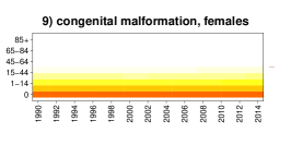
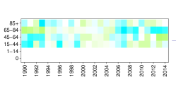
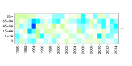
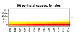
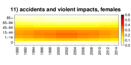
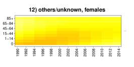
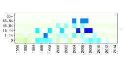
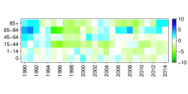
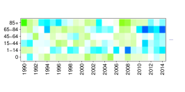
Figure 5: The odd rows illustrate the regression tree estimated probabilities $\theta^{\text{tree}}(k|{\bm{x}})$ for females. These plots all have the same scale given in the middle plot in each odd row. The even rows show the corresponding Pearson’s residuals given by (4.3). These plots all have the same scale given in the middle plot in each even row.

 

 

 

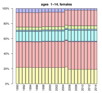
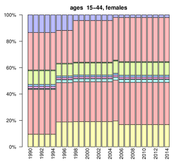
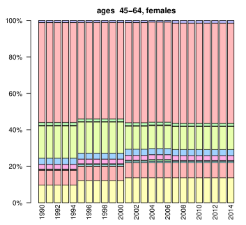
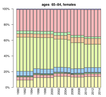
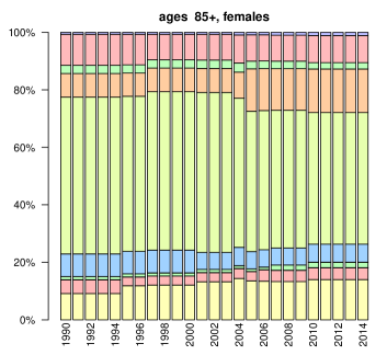
Figure 7: Regression tree estimated probabilities $\theta^{\text{tree}}(k|{\bm{x}})$ for females and for the $12$ different causes of death considered.

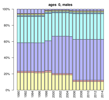
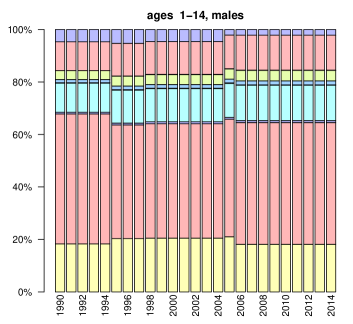
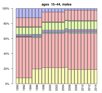
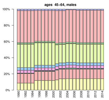
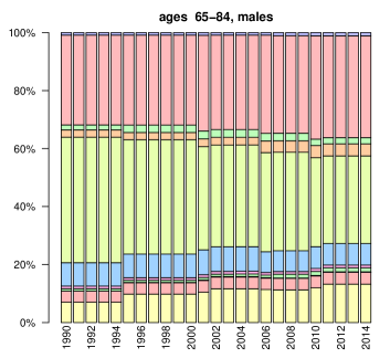
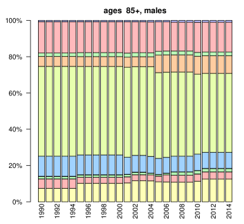
Figure 8: Regression tree estimated probabilities $\theta^{\text{tree}}(k|{\bm{x}})$ for males and for the $12$ different causes of death considered.

References

- [1] D. H. Alai, S. Arnold(-Gaille), and M. Sherris. Modelling cause-of-death mortality and the impact of cause-elimination. Annals of Actuarial Science, 9(1):167–186, 2015.
- [2] L. Breiman, J. Friedman, R. A. Olshen, and C. J. Stone. Classification and Regression Trees. Wadsworth Statistics/Probability Series, 1984.
- [3] A. J. G. Cairns, D. Blake, K. Dowd, G. D. Coughlan, D. Epstein, A. Ong, and I. Balevich. A quantitative comparison of stochastic mortality models using data from England and Wales and the United States. North American Actuarial Journal, 13(1):1–35, 2009.
- [4] J. Hirz, U. Schmock, and P. Shevchenko. Crunching mortality and life insurance portfolios with extended CreditRisk+. Risk Magazine, pages 98–103, 2017.
- [5] R. D. Lee and L. R. Carter. Modeling and forecasting U.S. mortality. Journal of the American Statistical Association, 87(419):659–671, 1992.
- [6] A. E. Renshaw and S. Haberman. Lee-Carter mortality forecasting: A parallel generalized linear modelling approach for England and Wales mortality projections. Journal of the Royal Statistical Society. Series C (Applied Statistics), 52(1):119–137, 2003.
- [7] A. E. Renshaw and S. Haberman. A cohort-based extension to the Lee-Carter model for mortality reduction factors. Insurance: Mathematics and Economics, 38(3):556–570, 2006.
- [8] S. J. Richards. Selected issues in modelling mortality by cause and in small populations. British Actuarial Journal, 15(supplement):267–283, 2009.
- [9] H. Stommel and E. Stommel. Volcano Weather: the Story of 1816, the Year Without a Summer. Seven Seas Press, 1983.
- [10] T. M. Therneau, E. J. Atkinson, and M. Foundation. An introduction to recursive partitioning using the RPART routines. R Vignettes, version of June 29, 2015.
- [11] A. M. Villegas, P. Millossovich, and V. Kaishev. StMoMo: an R package for stochastic mortality modelling. R Vignettes, version of February 9, 2016.
- [12] M. V. Wüthrich. Non-life insurance: mathematics & statistics, 2016. Available at https://ssrn.com/abstract=2319328.
- [13] M. V. Wüthrich and C. Buser. Data analytics for non-life insurance pricing, 2016. Available at https://ssrn.com/abstract=2870308.