The effect of finite-conductvity Hartmann walls on the linear stability of Hunt’s flow

Abstract

We analyse numerically the linear stability of the fully developed liquid metal flow in a square duct with insulating side walls and thin electrically conducting horizontal walls with the wall conductance ratio $c=0.01\cdots 1$ subject to a vertical magnetic field with the Hartmann numbers up to $\mathit{Ha}=10^{4}.$ In a sufficiently strong magnetic field, the flow consists of two jets at the side walls walls and a near-stagnant core with the relative velocity $\sim(c\mathit{Ha})^{-1}$. We find that for $\mathit{Ha}\gtrsim 300,$ the effect of wall conductivity on the stability of the flow is mainly determined by the effective Hartmann wall conductance ratio $c\mathit{Ha}.$ For $c\ll 1$, the increase of the magnetic field or that of the wall conductivity has a destabilizing effect on the flow. Maximal destabilization of the flow occurs at $\mathit{Ha}\approx 30/c$. In a stronger magnetic field with $c\mathit{Ha}\gtrsim 30$, the destabilizing effect vanishes and the asymptotic results of Priede et al. [J. Fluid Mech. 649, 115, 2010] for the ideal Hunt’s flow with perfectly conducting Hartmann walls are recovered.

1 Introduction

Some tokamak-type nuclear fusion reactors, which are expected to provide virtually unlimited amount of safe energy in the future, contain blankets made of rectangular ducts in which liquid metal flows in a high, transverse magnetic field between $5\,\mathrm{T}$ and $10\,\mathrm{T}$ (Bühler, 2007). These blankets are designed to cool the plasma chamber, to breed and to remove tritium as well as to protect the superconducting magnetic field coils from the neutron radiation emitted by the fusion plasma. The transfer properties of the magnetohydrodynamic flows depend strongly on their stability. On the one hand, magnetohydrodynamic instabilities and the associated turbulent mixing can enhance the transport of heat and mass, which is beneficial for the cooling and removal of tritium. On the other hand, it can also enhance the transport of momentum, which has an adverse effect on the hydrodynamic resistance of the duct (Zikanov et al., 2014).

Linear stability of MHD flows strongly varies with the electrical conductivity of the duct walls. In the duct with perfectly conducting walls, where the flow has weak jets along the walls parallel to the magnetic field (Uflyand, 1961; Chang & Lundgren, 1961), the critical Reynolds number based on the maximum flow velocity increases asymptotically as $\mathit{Re}_{c}\sim 642\mathit{Ha}^{1/2},$ where the Hartmann number $\mathit{Ha}$ defines the strength of the applied magnetic field (Priede et al., 2012). In the duct made of thin conducting walls, where strong side-wall jets carry a significant fraction of the volume flux (Walker, 1981), the flow becomes unstable at a substantially lower maximal velocity corresponding to $\mathit{Re}_{c}\sim 110\mathit{Ha}^{1/2}$ (Priede et al., 2015). Even more unstable is the so-called Hunt’s flow (Hunt, 1965), which develops when the walls parallel to the magnetic field are insulating whereas the perpendicular walls, often referred to as the Hartmann walls, are perfectly conducting. In this case the side-wall jets carry dominant part of the volume flux, and the asymptotic instability threshold drops to $\mathit{Re}_{c}\sim 90\mathit{Ha}^{1/2}$ (Priede et al., 2010).

Hunt’s flow is conceptually simple but like the flow in perfectly conducting duct it is rather far from reality where the walls usually have a finite electrical conductivity. Therefore it is of practical importance to consider the effect of finite electrical conductivity of Hartmann walls on the experimentally viable Hunt’s flow. This is the main focus of the present study which is concerned with linear stability analysis of the imperfect Hunt’s flow with thin finite conductivity Hartmann walls.

The paper is organised as follows. The problem is formulated in $\S$2. Numerical results for a square duct are presented in $\S$3. The paper is concluded with a summary and discussion of results in $\S$4.

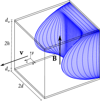
Figure 1: The base flow profile in a square duct with insulating side walls and thin conducting horizontal walls with the wall conductance ratio $c=0.1$ subject to a vertical magnetic field with $\textit{$\mathit{Ha}$}=100.$

2 Formulation of the problem

Consider the flow of an incompressible viscous electrically conducting liquid in a duct with half width $d$ and half height $h$ inside a transverse homogeneous magnetic field $\mathit{B}$. The point of origin is at the centre of the duct with axis orientation as shown in figure 1. The liquid flow is governed by the Navier-Stokes equation

$$\partial_{t}\mbox{\boldmath$\mathit{v}$}+(\mbox{\boldmath$\mathit{v}$}\cdot\mbox{\boldmath$\mathit{\nabla}$})\mbox{\boldmath$\mathit{v}$}=-\rho^{-1}\mbox{\boldmath$\mathit{\nabla}$}p+\nu\mbox{\boldmath$\mathit{\nabla}$}^{2}\mbox{\boldmath$\mathit{v}$}+\rho^{-1}\mbox{\boldmath$\mathit{f}$},$$ (1)

with the electromagnetic body force $\mbox{\boldmath$\mathit{f}$}=\mbox{\boldmath$\mathit{j}$}\times\mbox{\boldmath$\mathit{B}$}$ involving the induced electric current $\mbox{\boldmath$\mathit{j}$},$ which is governed by the Ohm’s law for a moving medium

$$\mbox{\boldmath$\mathit{j}$}=\sigma(\mbox{\boldmath$\mathit{E}$}+\mbox{\boldmath$\mathit{v}$}\times\mbox{\boldmath$\mathit{B}$}).$$ (2)

The flow is assumed to be sufficiently slow for the induced magnetic field to be negligible relative to the imposed one. This corresponds to the so-called inductionless approximation which holds for small magnetic Reynolds numbers $\mathit{Rm}=\mu_{0}\sigma v_{0}d\ll 1,$ where $\mu_{0}$ is the permeability of free space and $v_{0}$ is a characteristic velocity of the flow. In addition, we assume the characteristic time of velocity variation to be much longer than the magnetic diffusion time $\tau_{m}=\mu_{0}\sigma d^{2}.$ This is known in MHD as the quasi-stationary approximation (Roberts, 1967), which leads to $\mbox{\boldmath$\mathit{E}$}=-\mbox{\boldmath$\mathit{\nabla}$}\phi,$ where $\phi$ is the electrostatic potential.

Velocity and current satisfy mass and charge conservation $\mbox{\boldmath$\mathit{\nabla}$}\cdot\mbox{\boldmath$\mathit{v}$}=0,\mbox{\boldmath$\mathit{\nabla}$}\cdot\mbox{\boldmath$\mathit{j}$}=0.$ Applying the latter to Ohm’s law (2) and using the inductionless approximation, we obtain

$$\mbox{\boldmath$\mathit{\nabla}$}^{2}\phi=\mbox{\boldmath$\mathit{B}$}\cdot\mbox{\boldmath$\mathit{\omega}$},$$ (3)

where $\mbox{\boldmath$\mathit{\omega}$}=\mbox{\boldmath$\mathit{\nabla}$}\times\mbox{\boldmath$\mathit{v}$}$ is the vorticity. At the duct walls $S$, the normal $(n)$ and tangential $(\tau)$ velocity components satisfy the impermeability and no-slip boundary conditions $\left.v_{n}\right|_{s}=0$ and $\left.v_{\tau}\right|_{s}=0.$ Charge conservation applied to the thin wall leads to the following boundary condition

$$\left.\partial_{n}\phi-dc\mbox{\boldmath$\mathit{\nabla}$}_{\tau}^{2}\phi\right|_{s}=0,$$ (4)

where $c=\sigma_{w}d_{w}/(\sigma d)$ is the wall conductance ratio (Walker, 1981). At the non-conducting side walls with $c=0$ we have $\partial_{n}\phi|_{s}=0$.

The problem admits a rectilinear base flow along the duct with $\bar{\mbox{\boldmath$\mathit{v}$}}=(0,0,\bar{w}(x,y)),$ which is computed numerically and then analysed for the linear stability using a vector streamfunction-vorticity formulation introduced by Priede et al. 2010 which briefly outlined in the Appendix.

3 Results

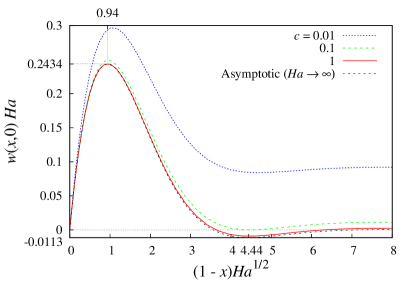
Figure 2: Horizontal base flow velocity profiles at $y=0$ in the vicinity of the side-wall in stretched coordinate $(1-x)\mathit{Ha}^{1/2}$ for various Hartmann wall conductance ratios $c$ and $\mathit{Ha}=10^{3}.$

Let us first consider the principal characteristics of the base flow, which will be useful for interpreting its stability later. Although rectangular duct with insulating side walls and thin conducting Hartmann walls admits an analytical Fourier series solution, (Hunt, 1965) it is more efficient to compute the base flow numerically (Priede et al., 2010). On the other hand, the important properties of the base flow can be deduced from the general asymptotic solution derived by Priede et al. (2015) for arbitrary Hartmann and side wall conductane ratios $c_{n}$ and $c_{\tau}.$ Below we provide the relevant results which follow from the general solution for the case of Hunt’s flow with thin Hartmann walls $(c_{n}=c>0)$ and insulating side walls $(c_{\tau}=0).$ According to the asymptotic solution, the conductivity of Hartmann walls affects primarily the flow in the core region of the duct. In a sufficiently strong magnetic satisfying $c\mathit{Ha}\gg 1,$ the core velocity scales as

$$\bar{w}_{\infty}\sim-(1+c^{-1})\mathit{Ha}^{-2}\bar{P}.$$ (5)

Velocity distribution at the side walls can written as

$$\bar{w}_{0}(\tilde{x},y)=\bar{w}_{\infty}[1+\sum_{k=0}^{\infty}e^{-\lambda\tilde{x}}B\left[C\sin(\lambda\tilde{x})+\cos(\lambda\tilde{x})\right]\cos(\kappa y)],$$ (6)

where $\tilde{x}=\mathit{Ha}^{1/2}(A\pm x)$ is a stretched side-layer coordinate and $A=h/d$ is the aspect ratio; $\kappa=\pi(k+1/2),$ $\lambda=\sqrt{\kappa/2},$ $B=(-1)^{k+1}2/\kappa$ and $C=-\mathit{Ha}^{-1}\bar{P}/(\bar{w}_{\infty}\kappa)$ are coefficients which depend on the summation index $k$. For $c\mathit{Ha}\gg 1$, the conductivity of Hartmann walls has virtually no effect on the velocity distribution (6), which reduces to that of the ideal Hunt’s flow with the maximal jet velocity

$$\bar{w}_{\max}\sim-0.2434\mathit{Ha}^{-1}\bar{P},$$ (7)

which is located at the distance $\delta\sim 0.94\mathit{Ha}^{-1/2}$ from the side wall (see Fig. 2). As seen, the velocity of jets is much higher than that of the core if $\mathit{Ha}\gg 1+c^{-1}.$ For poorly conducting Hartmann walls with $c\ll 1$, this is condition reduces to $c\mathit{Ha}\gg 1.$ It is the same condition that underlies (5) and means that the Hartmann walls are well conducting relative to the adjacent Hartmann layers. In this the case, the velocity of core flow scales as $\sim(c\mathit{Ha})^{-1}$ relative to that of side-wall jets. It means that the effect of the core flow and, consequently, that of the conductivity of Hartmann walls on the stability of Hunt’s flow is expected to vanish when the jet velocity is used to parametrize the problem.

The volume flux carried by the side-wall jets in a quarter duct cross-section is

$$q=\mathit{Ha}^{-1/2}\int_{0}^{\infty}\int_{0}^{1}\left(\bar{w}_{0}(\tilde{x},y)-\bar{w}_{\infty}\right)\mathrm{d}y\thinspace\mathrm{d}\tilde{x}\sim\alpha\mathit{Ha}^{-3/2}\bar{P},$$

where $\alpha=(16-\sqrt{2})\pi^{-7/2}\zeta(\frac{7}{2})\approx 0.299$ and $\zeta(x)$ is the Riemann zeta function (Abramowitz & Stegun, 1972). The respective fraction of the volume flux carried by the side-wall jets is

$$\gamma\sim\frac{q}{q+\bar{w}_{\infty}A}=\left(1+A\alpha^{-1}(1+c^{-1})\mathit{Ha}^{-1/2}\right)^{-1}.$$

The expression above is confirmed by the numerical results plotted in figure 3(a), where the curves for different wall conductance ratios are seen to collapse to this asymptotic solution when plotted against the modified Hartmann number $\mathit{Ha}/(1+c^{-1})^{2}.$ It implies that a strong magnetic field with $\mathit{Ha}\gg c^{-2}$ is required for the side-wall jets to fully develop, that is to carry the dominant fraction of the volume flux $\gamma\rightarrow 1$ in the non-ideal Hunt’s flow with weakly conducting Hartmann walls $(c\ll 1).$ This is confirmed also by the total volume flux plotted in figure 3(b) for the base flow normalized with the maximal velocity, which we use as the characteristic velocity in this study. The curves for different conductance ratios are seen to collapse to the asymptotic solution

$$Q=(q+\bar{w}_{\infty}A)/\bar{w}_{\max}\sim(1.229+4.109(1+c^{-1})\mathit{Ha}^{-1/2})\mathit{Ha}^{-1/2}$$ (8)

when $\mathit{Ha}/(1+c^{-1})^{2}\gg 1.$ This shows that a much stronger magnetic field is required to attain the asymptotic regime in the non-ideal Hunt’s flow when the volume flux rather than the jet velocity is used to parametrise the problem. It is due to the much larger area of the core region, which scales as $\sim\mathit{Ha}^{1/2}$ relative to that of the side-wall jets and thus makes the fraction of the volume flux carried by the core flow $\sim 1/(c\mathit{Ha}^{1/2}).$ Therefore it is advantageous to use the maximal rather than the mean velocity as a characteristic parameter. In this way, the high-field asymptotics of critical parameters can be extracted from the numerical solution at significantly lower Hartmann numbers. One can use the volume flux plotted in figure 3(a) or the asymptotic expression ((8)), if the magnetic field is sufficiently strong, to convert from our Reynolds number based on the maximal velocity to that based on the mean velocity.

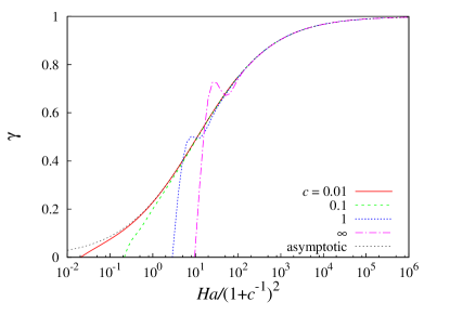
Figure 3: The volume flux fraction $\gamma$ carried by the side-wall jets for different wall conductance ratios $c$ (a) and the rescaled total volume flux $Q\mathit{Ha}^{1/2}$ (b) versus the modified Hartmann number $\mathit{Ha}/(1+c^{-1})^{2}$ for the base flow normalized with the maximal jet velocity; $c=\infty$ corresponds to the ideal Hunt’s flow with perfectly conducting Hartmann walls.

Now let us turn to the stability of the flow in a square duct $(A=1)$ and start with moderately conducting Hartmann walls with $c=1,$ which is used in the following unless stated otherwise. The marginal Reynolds number, at which the growth rate of different instability modes turns zero are plotted against the wavenumber in figure 4. The minimum on each marginal Reynolds number curve defines a critical wavenumber and the respective Reynolds number $\mathit{Re}_{c}$ by exceeding which the flow becomes unstable with respect to the perturbation of the given symmetry for the specified Hartmann number. Other critical points for different instability modes and Hartmann numbers are marked by dots in figure 4 and plotted explicitly against the Hartmann number in figure 5 with solid lines for $c=1$ and with dashed lines for other wall conductivity ratios. For $c=1,$ figure 5 shows critical parameters for all four instability modes. For other wall conductance ratios, only the critical parameters for the most unstable modes, i.e. those with the lowest $\mathit{Re}_{c}$ for the given $\mathit{Ha},$ are plotted. Figure 5 (a) shows that for $c=1,$ a magnetic field with $\mathit{Ha}\gtrsim 8$ is required for the flow in square duct to become linearly unstable. The first instability mode is of type II, which is typical for the MHD duct flows. Critical Reynolds number for this mode reaches minimum $\mathit{Re}_{c}\approx 12000$ at $\mathit{Ha}\approx 13$ and then starts to increase with the magnetic field. In a high magnetic field, the increase of critical Reynolds number is close to $\mathit{Re}_{c}\sim\mathit{Ha}.$

At $\mathit{Ha}\gtrsim 25,$ an instability mode of symmetry type IV appears with a critical Reynolds number significantly higher than that for the mode II. Critical Reynolds number for this mode attains minimum $\mathit{Re}_{c}\approx 17000$ at $\mathit{Ha}\approx 50$ and then stays slightly below $\mathit{Re}_{c}$ for mode II at larger $\mathit{Ha}.$ These two instability modes are efficiently stabilized by a sufficiently strong magnetic field which leads to $\mathit{Re}_{c}$ increasing nearly linearly with $\mathit{Ha}.$ This is due to the anti-symmetric vertical distribution of the $y$-component of vorticity (see table 2), which makes it essentially non-uniform along the magnetic field and thus subject to a strong magnetic damping.

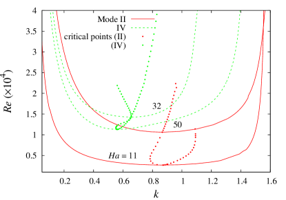
Figure 4: Marginal Reynolds numbers for modes II,IV (a)and I,III (b) depending on wavenumber $k$ for $c=1$. The dots indicate critical points for other Hartmann numbers.

Two additional instability modes – one of type I and another of type III – emerge at $\mathit{Ha}\approx 50.$ These two modes have similar critical Reynolds numbers, which are seen in figure 5(a) to quickly drop below those for modes II and IV. This makes modes I and III the most unstable ones in a sufficiently strong magnetic field. The critical wavenumbers for modes I and III are practically indistinguishable one from another in figure 5(b). As seen in figure 4(b), at moderate Hartmann numbers $\mathit{Ha}\approx 70$ modes I and III may have intricate neutral stability curves which of consist of closed contours and disjoint open parts. For $\mathit{Ha}=70,$ mode III has not one but three critical Reynolds numbers. By exceeding the lowest $\mathit{Re}_{c}$ the flow becomes unstable and remains such up to the second $\mathit{Re}_{c},$ above which it restabilizes. After that the flow remains stable up to the third $\mathit{Re}_{c},$ above which it turns ultimately unstable. As seen in figure 5(a), such a triple stability threshold for modes I/III, which are shown by dots for mode III at $\mathit{Ha}=70$, exists only in a relative narrow range of Hartmann numbers around $\mathit{Ha}\approx 70.$

The lowest critical Reynolds number for modes I and III, $\mathit{Re}_{c\ }\approx 1300$ is attained at $\mathit{Ha}\approx 100.$ In a high magnetic field, the critical Reynolds numbers and wavenumbers for both modes increase asymptotically as $\mathit{Re}_{c}\sim k_{c}\sim\mathit{Ha}^{1/2}$ , which means that the relevant length scale of instability is determined by the thickness of the side layers $\delta\sim\mathit{Ha}^{-1/2}.$

The much weaker magnetic damping of modes I/III in comparison to modes II/IV is due to the symmetric (even) vertical distribution of the $y$-component of vorticity which makes it relatively uniform along the magnetic field. The spanwise symmetry, which is opposite for modes I and III, and determines the relative sense of rotation of vertical vortices at the opposite side walls, has almost no effect on their stability in a sufficiently strong magnetic field, where the critical parameters for both modes become virtually identical.

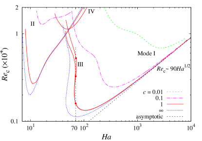
Figure 5: Critical Reynolds number (a), wavenumber (b) and the relative phase velocity (c) against the Hartmann number for different wall conductance ratios $c$; $c=\infty$ corresponds to the ideal Hunt’s flow considered by Priede et al. (2010).

Now let us consider the stability of the flow at lower wall conductance ratios. As seen in figure 5(a), the critical Reynolds number increases, which means that the flow becomes more stable, when the wall conductivity is reduced provided that the magnetic field is not too strong. In a strong magnetic field, this stabilizing effect vanishes and the curves for different wall conductance ratios collapse to the asymptotics of the ideal Hunt’s flow with $\mathit{Re}_{c}\sim 90\mathit{Ha}^{1/2},$ $k_{c}\sim 0.525\mathit{Ha}^{1/2}$ and $-\omega_{c}/(\mathit{Re}_{c}k_{c})\approx 0.475$ found by Priede et al. (2010).

As discussed at the beginning of this section, $\mathit{Ha}\gg c^{-1}$ is required for these asymptotics. This estimate is consistent with the Hartmann numbers at which the lowest critical Reynolds numbers are attained for different wall conductance ratios (see table 1). A more specific confirmation of this estimate may be seen in figure 6(a), where the rescaled critical Reynolds numbers $\mathit{Re}_{c}/\mathit{Ha}^{1/2}$ collapse for different $\mathit{Ha}\gtrsim 300$ to nearly the same curve when plotted against the rescaled wall conductance ratio $c\mathit{Ha}.$ Also the rescaled critical wavenumber $k_{c}/\mathit{Ha}^{1/2}$ is seen in figure 6(b) to collapse in a similar way for $c\mathit{Ha}\gtrsim 10.$ The latter parameter combination represents an effective wall conductance ratio which defines the wall conductance relative to that of the adjacent Hartmann layer. A more detailed physical interpretation of $c\mathit{Ha}$ will be given in the conclusion. Figure 6 shows that in a strong magnetic field with $\mathit{Ha}\gtrsim 300,$ the effect of wall conductivity on the stability of flow is mainly determined by a single parameter, the effective wall conductance ratio $c\mathit{Ha}.$ According to table 1, Hartmann walls with $c\ll 1$ have a stabilizing effect on the flow only up to $c\mathit{Ha}\gtrsim 30.$ At higher effective wall conductance ratios, as seen in figure 6, the high-field asymptotics of Hunt’s flow are recovered.

Figure 6: Rescaled critical Reynolds number $\mathit{Re}_{c}/\mathit{Ha}^{1/2}$ (a) and the wavenumber $k_{c}/\mathit{Ha}^{1/2}$ (b) against the rescaled wall conductance ratio $c\mathit{Ha}$ for different Hartmann numbers $\mathit{Ha}.$

$c$	$\mathit{Re}_{c}$	$\mathit{Ha}$
1	1300	100
0.1	2500	350
0.01	6900	2800

Table 1: The lowest critical Reynolds numbers $\mathit{Re}_{c}$ and the corresponding Hartmann numbers for different wall conductance ratios $c$

4 Summary and Conclusions

We have investigated numerically the linear stability of a realistic Hunt’s flow in a square duct with finite conductivity Hartmann walls and insulating side walls subject to a homogeneous vertical magnetic field. It was found that in a sufficiently strong magnetic field with $\mathit{Ha}\gtrsim 300$ the impact of wall conductivity on the stability of the flow is determined mainly by a single parameter – the effective Hartmann wall conductance ratio $c\mathit{Ha}$. This parameter characterizes the wall conductance relative to that of the adjacent Hartmann layer, which is connected electrically in parallel to the former. Because the thickness and, thus, also the conductance of Hartmann layer drops inversely with the applied magnetic field, a finite conductivity wall becomes relatively well conducting in the sufficiently strong magnetic field.

There are two reasons why $c\mathit{Ha}$ emerges as the relevant stability parameter of Hunt’s flow with finite-conductivity Hartmann walls. Firstly, it is due to the core region of the base flow, whose velocity in a sufficiently strong magnetic field scales according to (5) as $\sim(c\mathit{Ha})^{-1}$ relative to that of the side-wall jets (7) when the wall conductance ratio is small $(c\ll 1)$. Secondly, $c\mathit{Ha}$ plays the role of effective wall conductance ratio in the thin-wall boundary condition (4) and replaces $c$ when the side-wall jet thickness $\delta\sim\mathit{Ha}^{-1/2}$ is used as the effective horizontal length scale of instability in the $(x,z)$ plane.

We found that the conductivity of Hartmann walls has a significant stabilizing effect on the flow as long as $c\mathit{Ha}\lesssim 30.$ Since the instability originates in the side-wall jets with the characteristic thickness $\delta\sim\mathit{Ha}^{-1/2},$ the critical Reynolds number scales as $\mathit{Re}_{c}\sim\mathit{Ha}^{1/2}\tilde{\mathit{Re}}_{c}(c\mathit{Ha}),$ where $\tilde{\mathit{Re}}_{c}$ is a rescaled critical Reynolds number which depends mainly on $c\mathit{Ha}$ and varies very little with $\mathit{Ha}.$ A similar relationship holds also for the critical wavenumber $k_{c}\sim\mathit{Ha}^{1/2}\tilde{k}_{c}(c\mathit{Ha}),$ where the rescaled wavenumber $\tilde{k}_{c}$ starts depend directly on $\mathit{Ha}$ if $c\mathit{Ha}\lesssim 10.$ This is likely due to the effect of the core flow, which has the relative velocity $\sim(c\mathit{Ha})^{-1}$, and thus may be no longer negligible with respect to the jet velocity if $c\mathit{Ha}\lesssim 10.$ In the strong magnetic field satisfying $c\mathit{Ha}\gtrsim 30$, the stabilizing effect of wall conductivity vanishes, and the asymptotic solution $\tilde{\mathit{Re}}_{c}\approx 90$ and $\tilde{k}_{c}\approx 0.525$ found by Priede et al. (2010) for the ideal Hunt’s flow with perfectly conducting Hartmann walls is recovered. Consequently, for the Hartmann walls to become virtually perfectly conducting with respect to the stability of flow, the magnetic field with $\mathit{Ha}\gtrsim 30/c$ is required. Maximal destabilization of the flow, i.e., the lowest critical Reynolds number for the given wall conductance ratio, is achieved at $\mathit{Ha}\approx 30/c.$ This result suggests an optimal design of liquid metal blankets when efficient turbulent removal of heat from side walls is required. Note that a much stronger magnetic field with $\mathit{Ha}\gg c^{-2}$ is required for the volume flux carried by the side-wall jets to fully develop and become dominant as in the Hunt’s flow with perfectly conducting Hartmann walls. However, it is the local velocity distribution at the side walls which determines the stability of this type of flow. Therefore it is the relative velocity of the core flow rather than its volume flux which is relevant for the stability of Hunt’s flow.

In conclusion, it is important to note that the instability considered in this study corresponds to the so-called convective instability (Schmid & Henningson, 2012, Secs. 7.2.1–7.2.3). In contrast to the absolute instability, the convective one is not in general self-sustained and, thus, may not be directly observable in the experiments without external excitation. However, it should be observable in the direct numerical simulation using periodicity condition in the stream-wise direction. The absolute instability threshold, if any, is still unknown for this type of flow. But given the relatively low local critical Reynolds number $\tilde{\mathit{Re}}_{c}\sim 100,$ it is very likely to be relevant for such MHD duct flows with the side-wall jets.

Also the physical mechanism behind in the instability itself is not entirely clear. The low $\tilde{\mathit{Re}}_{c}$ as well as the presence of inflection points in the velocity profile imply that the instability could be inviscid, although the latter criterion is strictly applicable to one-dimensional inviscid flows only. The respective criteria of two-dimensional inviscid flows are considerably more complicated (Bayly et al., 1988), and no such criterion is known for MHD flows. A complicated numerical analysis may be required to answer this non-trivial question.

This work was supported by the Liquid Metal Technology Alliance (LIMTECH) of the Helmholtz Association. The authors are indebted to the Faculty of Engineering, Environment and Computing of Coventry University for the opportunity to use its high performance computer cluster.

5 Vector streamfunction-vorticity formulation

In order to satisfy the incompressibility constraint $\mbox{\boldmath$\mathit{\nabla}$}\cdot\mbox{\boldmath$\mathit{v}$}=0$, we introduce a vector streamfunction $\mathit{\psi}$ which allows us to seek the velocity distribution in the form $\mbox{\boldmath$\mathit{v}$}=\mbox{\boldmath$\mathit{\nabla}$}\times\mbox{\boldmath$\mathit{\psi}$}.$ Since $\mathit{\psi}$ is determined up to a gradient of arbitrary function, we can impose an additional constraint

$$\mbox{\boldmath$\mathit{\nabla}$}\cdot\mbox{\boldmath$\mathit{\psi}$}=0,$$ (9)

which is analogous to the Coulomb gauge for the magnetic vector potential $\mathit{A}$ (Jackson, 1998). Similar to the incompressibility constraint for $\mbox{\boldmath$\mathit{v}$},$ this gauge leaves only two independent components of $\mbox{\boldmath$\mathit{\psi}$}.$

The pressure gradient is eliminated by applying curl to (1). This yields two dimensionless equations for $\mathit{\psi}$ and $\mathit{\omega}$

$$\partial_{t}\mbox{\boldmath$\mathit{\omega}$} = \mbox{\boldmath$\mathit{\nabla}$}^{2}\mbox{\boldmath$\mathit{\omega}$}-\mathit{Re}\mbox{\boldmath$\mathit{g}$}+\mathit{Ha}^{2}\mbox{\boldmath$\mathit{h}$},$$ (10)

$$0 = \mbox{\boldmath$\mathit{\nabla}$}^{2}\mbox{\boldmath$\mathit{\psi}$}+\mbox{\boldmath$\mathit{\omega}$},$$ (11)

where $\mbox{\boldmath$\mathit{g}$}=\mbox{\boldmath$\mathit{\nabla}$}\times(\mbox{\boldmath$\mathit{v}$}\cdot\mbox{\boldmath$\mathit{\nabla}$})\mbox{\boldmath$\mathit{v}$},$ and $\mbox{\boldmath$\mathit{h}$}=\mbox{\boldmath$\mathit{\nabla}$}\times\mbox{\boldmath$\mathit{f}$}$ are the curls of the dimensionless convective inertial and electromagnetic forces, respectively.

The boundary conditions for $\mathit{\psi}$ and $\mathit{\omega}$ were obtained as follows. The impermeability condition applied integrally as $\int_{s}\mbox{\boldmath$\mathit{v}$}\cdot\mbox{\boldmath$\mathit{ds}$}=\oint_{l}\mbox{\boldmath$\mathit{\psi}$}\cdot\mbox{\boldmath$\mathit{dl}$}=0$ to an arbitrary area of wall $s$ encircled by the contour $l$ yields $\left.\psi_{\tau}\right|_{s}=0.$ This boundary condition substituted into (9) results in $\left.\partial_{n}\psi_{n}\right|_{s}=0.$ In addition, applying the no-slip condition integrally $\oint_{l}\mbox{\boldmath$\mathit{v}$}\cdot\mbox{\boldmath$\mathit{\mathrm{d}l}$}=\int_{s}\mbox{\boldmath$\mathit{\omega}$}\cdot\mbox{\boldmath$\mathit{\mathrm{d}s}$}$ we obtain $\left.\omega_{n}\right|_{s}=0.$

The base flow can conveniently be determined using the $z$-component of the induced magnetic field $\bar{b}$ instead of the electrostatic potential $\bar{\phi}.$ Then the governing equations for the base flow take the form

$$\mbox{\boldmath$\mathit{\nabla}$}^{2}\bar{w}+\mathit{Ha}\partial_{y}\bar{b} = \bar{P,}$$ (12)

$$\mbox{\boldmath$\mathit{\nabla}$}^{2}\bar{b}+\mathit{Ha}\partial_{y}\bar{w} = 0,$$ (13)

where $\mathit{Ha}=dB\sqrt{\sigma/(\rho\nu)}$ is the Hartmann number and $\bar{b}$ is scaled by $\mu_{0}\sqrt{\sigma\rho\nu^{3}}/d.$ The constant dimensionless axial pressure gradient $\bar{P}$ that drives the flow is determined from the normalisation condition $\bar{w}_{\max}=1.$ The velocity satisfies the no-slip boundary condition $\bar{w}=0$ at $x=\pm 1$ and $y=\pm A,$ where $A=h/d$ is the aspect ratio, which is set equal to $1$ for the square cross-section duct considered in this study. The boundary condition for the induced magnetic field (Shercliff, 1956) at the Hartmann wall is

$$\bar{b}=c\partial_{n}\bar{b}.$$ (14)

and $\bar{b}=0$ for the side wall.

Linear stability of the base flow $\{\bar{\mbox{\boldmath$\mathit{\psi}$}},\bar{\mbox{\boldmath$\mathit{\omega}$}},\bar{\phi}\}(x,y)$ is analysed with respect to infinitesimal disturbances in the standard form of harmonic waves travelling along the axis of the duct

$$\{\mbox{\boldmath$\mathit{\psi}$},\mbox{\boldmath$\mathit{\omega}$},\phi\}(\mbox{\boldmath$\mathit{r}$},t)=\{\bar{\mbox{\boldmath$\mathit{\psi}$}},\bar{\mbox{\boldmath$\mathit{\omega}$}},\bar{\phi}\}(x,y)+\{\hat{\mbox{\boldmath$\mathit{\psi}$}},\hat{\mbox{\boldmath$\mathit{\omega}$}},\hat{\phi}\}(x,y)e^{\lambda t+\mathrm{i}kz},$$

where $k$ is a real wavenumber and $\lambda$ is, in general, a complex growth rate. This expression substituted into (10,11) results in

$$\lambda\hat{\mbox{\boldmath$\mathit{\omega}$}} = \mbox{\boldmath$\mathit{\nabla}$}_{k}^{2}\hat{\mbox{\boldmath$\mathit{\omega}$}}-\textit{Re}\hat{\mbox{\boldmath$\mathit{g}$}}+\textit{Ha}^{2}\hat{\mbox{\boldmath$\mathit{h}$}},$$ (15)

$$0 = \mbox{\boldmath$\mathit{\nabla}$}_{k}^{2}\hat{\mbox{\boldmath$\mathit{\psi}$}}+\hat{\mbox{\boldmath$\mathit{\omega}$}},$$ (16)

$$0 = \mbox{\boldmath$\mathit{\nabla}$}_{k}^{2}\hat{\phi}-\hat{\omega}_{\shortparallel},$$ (17)

where $\mbox{\boldmath$\mathit{\nabla}$}_{k}\equiv\mbox{\boldmath$\mathit{\nabla}$}_{\perp}+\mathrm{i}k\mbox{\boldmath$\mathit{e}$}_{z};$ $\shortparallel$ and $\perp$ respectively denote the components along and transverse to the magnetic field in the $(x,y)$-plane. Because of the solenoidality of $\hat{\mbox{\boldmath$\mathit{\omega}$}},$ we need only the $x$- and $y$-components of (15), which contain $\hat{h}_{\perp}=-\partial_{xy}\hat{\phi}-\partial_{\shortparallel}\hat{w},$ $\hat{h}_{\shortparallel}=-\partial_{\shortparallel}^{2}\hat{\phi}$ and

$$\hat{g}_{x} = k^{2}\hat{v}\bar{w}+\partial_{yy}(\hat{v}\bar{w})+\partial_{xy}(\hat{u}\bar{w})+\mathrm{i}2k\partial_{y}(\hat{w}\bar{w}),$$ (18)

$$\hat{g}_{y} = -k^{2}\hat{u}\bar{w}-\partial_{xx}(\hat{u}\bar{w})-\partial_{xy}(\hat{v}\bar{w})-\mathrm{i}2k\partial_{x}(\hat{w}\bar{w}),$$ (19)

where

$$\hat{u} = \mathrm{i}k^{-1}(\partial_{yy}\hat{\psi}_{y}-k^{2}\hat{\psi}_{y}+\partial_{xy}\hat{\psi}_{x}),$$ (20)

$$\hat{v} = -\mathrm{i}k^{-1}(\partial_{xx}\hat{\psi}_{x}-k^{2}\hat{\psi}_{x}+\partial_{xy}\hat{\psi}_{y}),$$ (21)

$$\hat{w} = \partial_{x}\hat{\psi}_{y}-\partial_{y}\hat{\psi}_{x}.$$ (22)

The boundary conditions are

$$\partial_{x}\hat{\phi}=\hat{\psi}_{y}=\partial_{x}\hat{\psi}_{x}=\partial_{x}\hat{\psi}_{y}-\partial_{y}\hat{\psi}_{x}=\hat{\omega}_{x}=0 x=\pm 1,$$ at (23)

$$\partial_{x}^{2}\hat{\phi}-k^{2}\hat{\phi}\mp c^{-1}\partial_{y}\hat{\phi}=\hat{\psi}_{x}=\partial_{y}\hat{\psi}_{y}=\partial_{x}\hat{\psi}_{y}-\partial_{y}\hat{\psi}_{x}=\hat{\omega}_{y}=0 y=\pm A,$$ at (24)

where the aspect ratio $A=h/d=1$ for the square cross-section duct considered in this study. The problem was solved using the same spectral collocation method as in our previous study (Priede et al., 2015).

Owing to the double reflection symmetry of the base flow with respect to the $x=0$ and $y=0$ planes, small-amplitude perturbations with different parities in $x$ and $y$ decouple from each other. This results in four mutually independent modes, which we classify as $(o,o),$ $(o,e),$ $(e,o),$ and $(e,e)$ according to whether the $x$ and $y$ symmetry of $\hat{\psi}_{x}$ is odd or even, respectively. Our classification of modes corresponds to the symmetries I, II, III, and IV used by Tatsumi & Yoshimura (1990) and Uhlmann & Nagata (2006) (see table 2). The symmetry allows us to solve the linear stability problem for each of four modes separately using only one quadrant of the duct cross-section. A more detailed description of the spatial structure of different instability modes can be found in Priede et al. (2015).

	I	II	III	IV
$\hat{\psi}_{x},\,\hat{\omega}_{x},\,\hat{v}:$	$(o,o)$	$(o,e)$	$(e,o)$	$(e,e)$
$\hat{w}:$	$(o,e)$	$(o,o)$	$(e,e)$	$(e,o)$
$\hat{\psi}_{z},\,\hat{\omega}_{z}:$	$(e,o)$	$(e,e)$	$(o,o)$	$(o,e)$
$\hat{\psi}_{y},\,\hat{\omega}_{y},\,\hat{u},\,\phi:$	$(e,e)$	$(e,o)$	$(o,e)$	$(o,o)$

Table 2: The $(x,y)$ parities of different variables for symmetries I, II, III and IV; $e$ - even, $o$ - odd

References

- Abramowitz & Stegun (1972) Abramowitz, M. & Stegun, I. A. 1972 Handbook of Mathematical Functions. New York: Dover.
- Bayly et al. (1988) Bayly, Bruce J, Orszag, Steven A & Herbert, Thorwald 1988 Instability mechanisms in shear-flow transition. Annu Rev Fluid Mech 20 (1), 359–391.
- Bühler (2007) Bühler, L. 2007 Magnetohydrodynamics: Historical Evolution and Trends, chap. Liquid Metal Magnetohydrodynamics for Fusion Blankets, pp. 171–194. Springer.
- Chang & Lundgren (1961) Chang, C. C. & Lundgren, Th. S. 1961 Duct flow in magnetohydrodynamics. ZAMP 12 (2), 100–114.
- Hunt (1965) Hunt, J. C. R. 1965 Magnetohydrodynamic flow in rectangular ducts. J. Fluid Mech. 21 (04), 577–590.
- Jackson (1998) Jackson, J. D. 1998 Classical Electrodynamics. Wiley.
- Priede et al. (2010) Priede, J., Aleksandrova, S. & Molokov, S. 2010 Linear stability of Hunt’s flow. J. Fluid Mech. 649, 115–134.
- Priede et al. (2012) Priede, J., Aleksandrova, S. & Molokov, S. 2012 Linear stability of magnetohydrodynamic flow in a perfectly conducting rectangular duct. J. Fluid Mech. 708, 111–127.
- Priede et al. (2015) Priede, J., Arlt, T. & Bühler, L. 2015 Linear stability of magnetohydrodynamic flow in a square duct with thin conducting walls. J. Fluid Mech. 788, 129–146.
- Roberts (1967) Roberts, P. H. 1967 An Introduction to Magnetohydrodynamics. London: Longmans.
- Schmid & Henningson (2012) Schmid, P. J. & Henningson, D. S. 2012 Stability and transition in shear flows. New York: Springer.
- Shercliff (1956) Shercliff, J. A. 1956 The flow of conducting fluids in circular pipes under transverse magnetic fields. J. Fluid Mech. 1 (06), 644–666.
- Tatsumi & Yoshimura (1990) Tatsumi, T. & Yoshimura, T. 1990 Stability of the laminar flow in a rectangular duct. J. Fluid Mech. 212, 437–449.
- Uflyand (1961) Uflyand, Ya. S. 1961 Flow stability of a conducting fluid in a rectangular channel in a transverse magnetic field. Soviet Physics: Technical Physics 5 (10), 1191–1193.
- Uhlmann & Nagata (2006) Uhlmann, M. & Nagata, M. 2006 Linear stability of flow in an internally heated rectangular duct. J. Fluid Mech. 551, 387–404.
- Walker (1981) Walker, J. S. 1981 Magneto-hydrodynamic flows in rectangular ducts with thin conducting walls. J. de Mécanique 20 (1), 79–112.
- Zikanov et al. (2014) Zikanov, O., Krasnov, D., Boeck, T., Thess, A. & Rossi, M. 2014 Laminar-turbulent transition in magnetohydrodynamic duct, pipe, and channel flows. Appl. Mech. Rev. 66 (3), 030802.