Finite Difference Methods for the generator of 1D asymmetric alpha-stable Lévy motions

Abstract

Several finite difference methods are proposed for the infinitesimal generator of 1D asymmetric $\alpha$-stable Lévy motions, based on the fact that the operator becomes a multiplier in the spectral space. These methods take the general form of a discrete convolution, and the coefficients (or the weights) in the convolution are chosen to approximate the exact multiplier after appropriate transform. The accuracy and the associated advantages/disadvantages are also discussed, providing some guidance on the choice of the right scheme for practical problems, like in the calculation of mean exit time for random processes governed by general asymmetric $\alpha$-stable motions.

AMS Mathematics Subject Classification 2000. 35R09, 60G51, 65N06

Keywords: Finite difference method, $\alpha$-stable Lévy processes, psudo-differential operator

1 Introduction

While most random dynamical systems studied during the past century are driven by Gaussian noise, nowadays many complex systems are modelled with the presence of non-Gaussian noise generated from even more exotic Lévy processes [23].

A Lévy process is a stochastic process with stationary and independent increments [1, 24]. As a generalisation of the well-known Wiener process (also called Brownian motion), a (scalar) Lévy process $\{X_{t}\}_{t\geq 0}$ is characterised by the Lévy-Khintchine theorem, which states that the characteristic function of $X_{t}$ can be written as $\mathbb{E}\big{(}\exp(i\xi X_{t})|X_{0}=0\big{)}=\exp\big{(}t\psi(\xi)\big{)}$. Here, $\psi$ takes the general form

$$\psi(\xi)=i\mu\xi-\frac{1}{2}q^{2}\xi^{2}+\int_{\mathbb{R}\setminus\{0\}}\big{(}e^{iy\xi}-1-iy\xi\mathbf{1}_{|y|\leq 1}\big{)}\nu({\rm d}y),$$ (1)

where $\mu\in\mathbb{R},q\geq 0$, $\mathbf{1}_{S}$ is the indicator function on the set $S$ and $\nu$ is the so called Lévy measure that satisfies the condition

$$\int_{\mathbb{R}\setminus\{0\}}\min(1,y^{2})\ \nu({\rm d}y)<\infty.$$

Intimately related to a Lévy process is its infinitesimal generator $\mathcal{A}$, defined for a smooth function $f$ as

$$\mathcal{A}f(x):=\lim_{t\to 0^{+}}\frac{\mathbb{E}\big{(}f(X_{t})\mid X_{0}=x\big{)}-f(x)}{t}.$$

If $X_{t}$ is a Lévy process starting from $x$ at time $t=0$, then $\mathbb{E}\big{(}\exp(i\xi(X_{t}-x))|X_{0}=x\big{)}=\exp(t\psi(\xi))$, and the generator $\mathcal{A}f$ can also be represented as [5]

$$\mathcal{A}f(x)=\mu f^{\prime}(x)+\frac{q^{2}}{2}f^{\prime\prime}(x)+\int_{\mathbb{R}\setminus\{0\}}\big{[}f(x+y)-f(x)-y\mathbf{1}_{|y|\leq 1}f^{\prime}(x)\big{]}\ \nu({\rm d}y).$$ (2)

If the Fourier transform of $f$ is defined to be $\hat{f}(\xi)=\mathcal{F}[f](\xi)=\int_{\mathbb{R}}f(x)\exp(-i\xi x){\rm d}\xi$, then $\mathcal{A}$ becomes a multiplier in the spectral space, i.e.,

$$\widehat{\mathcal{A}f}(\xi)=\psi(-\xi)\hat{f}(\xi).$$

This operator $\mathcal{A}$ plays a similar role as the adjoint of the classical Fokker-Plank operator associated with systems driven by Brownian motions, and appears in the governing non-local differential equations for quantities that characterise the underlying stochastic processes. For instance, the mean exit time $u(x)$ for the expect time of a particle starting at $x$ and leaving the domain $\Omega$ satisfies the equation

$$\mathcal{A}u=-1\qquad\mbox{ on }\ \Omega,$$

with the boundary condition $u=0$ on $\Omega^{c}$. The adjoint operator $\mathcal{A}^{*}$ also arises in other contexts, like the evolution of the probability density distribution and escape probability [5].

In the modelling of practical problems driven by non-Gaussian noise, the final Lévy process usually appears as the limit of many small Lévy processes [24], giving rise to $\alpha$-stable Lévy processes that enjoy better scaling properties. In these new processes, the Lévy measure is simply

$$\nu({\rm d}y)=\frac{C_{+}\chi_{(0,\infty)}(y)+C_{-}\chi_{(-\infty,0)}(y)}{|y|^{1+\alpha}}({\rm d}y),$$ (3)

for some non-negative constants $C_{+}$ and $C_{-}$, and the stability parameter $\alpha\in(0,2)$. Using special integrals (22) in Appendix B, $\psi(t)$ defined in (1) becomes

$$\psi(t)=i(\mu+K)\xi-\frac{1}{2}q^{2}\xi^{2}+\Gamma(-\alpha)C_{+}(-i\xi)^{\alpha}+\Gamma(-\alpha)C_{-}(i\xi)^{\alpha}$$ (4)

where

$$K=\begin{cases}(C_{-}-C_{+})/(1-\alpha),\qquad&\alpha\neq 1,\cr(1-\gamma)(C_{+}-C_{-}),&\alpha=1,\end{cases}$$

and $\gamma(\approx 0.57721)$ is the Euler-Mascheroni constant. By isolating the real and imaginary parts, the function $\psi(t)$ in (4) can be written in the following form commonly seen in the literature

$$\psi(\xi)=i(\mu+K)\xi-\frac{1}{2}q^{2}\xi^{2}-\sigma^{\alpha}|\xi|^{\alpha}\big{(}1-i\beta\mbox{sgn}(\xi)\tan{({\pi\alpha}/2)}\big{)},$$ (5)

with the scaling parameter $\sigma>0$, the skewness parameter $\beta\in[-1,1]$. The constants in (4) and (5) are related by

$$C_{+}=C_{\alpha}\frac{1+\beta}{2},\quad C_{-}=C_{\alpha}\frac{1-\beta}{2},\qquad-1\leq\beta\leq 1,$$ (6)

with

$$C_{\alpha}=-\frac{\sigma^{\alpha}}{\Gamma(-\alpha)\cos{({\pi\alpha}/2)}}.$$ (7)

This connection between (3) and (4) turns out to motivate a particular type of finite difference schemes originated from fractional derivatives [9, 10].

Parallel to the progress made in the theoretical study of Lévy processes [1], related fields have been heavily investigated during the past two decades, including random simulations of these more exotic processes [16] and numerical approximations of the underlying non-local differential equations for quantities like the mean exit time and escape probability [5]. Numerous schemes have also been proposed to discretize these more complicated integro-differential equations, like those originated from random walk models [8, 9, 10] with fractional derivatives [3], those based on quadrature of the singular integral representation [4, 7, 13, 26] and harmonic extension [19].

In this paper, several finite difference schemes for the infinitesimal generator $\mathcal{A}$ will be constructed, by exploring their representations in the appropriate spectral space. For simplicity, only the normalised operator corresponding to

$$\widehat{\mathcal{A}}=\psi(-\xi)=\begin{cases}-|\xi|^{\alpha}\big{(}1+i\beta\operatorname{sgn}(\xi)\tan({\alpha\pi}/{2})\big{)},\qquad&\alpha\neq 1,\cr-|\xi|\big{(}1+i2\beta\operatorname{sgn}(\xi)\ln|\xi|/\pi\big{)},&\alpha=1,\end{cases}$$

will be considered; general cases can be adapted easily by adding discretization of classical first or second order derivatives for convection (if $\mu\neq 0$) or diffusion (if $q\neq 0$), and by applying appropriate scaling (if $\sigma\neq 1$). To motivate the general form of the schemes, basic theoretical tools related to semi-discrete Fourier transform will be reviewed in Section 2. In Section 3, specific schemes are constructed based on the approximate multipliers in the spectral space, followed by several numerical experiments in Section 4. Finally, special functions and integrals, as well as lengthy derivations of the weights in certain schemes are collected in the appendix.

2 The discrete operator and semi-discrete Fourier transform

For local operators like classical integer order derivatives, Taylor expansion is usually employed to derive difference schemes and to assess their order of accuracy. However, for nonlocal operators like fractional order derivatives [20] and infinitesimal generators like $\mathcal{A}$ above, local expansions around the point of interest soon become inadequate. The right theoretical framework has to be built upon new tools, like the semi-discrete Fourier transform for functions defined on a uniform infinite lattice.

Let $v$ be a discrete function (usually sampled from a continuous one) defined on the grid $\mathbb{Z}_{h}=\{x_{j}=hj\mid j\in\mathbb{Z}\}$ with uniform spacing $h$. Then its semi-discrete Fourier transform is defined as

$$\hat{v}(\xi)=\mathcal{F}[v](\xi)=h\sum_{j=-\infty}^{\infty}e^{-i\xi x_{j}}v_{j},\qquad\xi\in I_{h}:=\left[-\frac{\pi}{h},\frac{\pi}{h}\right].$$ (8)

Here the domain is restricted to be the finite interval $I_{h}$, as $\hat{v}$ is periodic with period $2\pi/h$. The inverse transform can also be readily worked out as

$$v_{j}=\mathcal{F}^{-1}[\hat{v}](x_{j})=\frac{1}{2\pi}\int_{-\pi/h}^{\pi/h}e^{i\xi x_{j}}\hat{v}(\xi){\rm d}\xi.$$ (9)

When the grid size $h$ goes to zero, both (8) and (9) converge to the continuous Fourier transform and inverse Fourier transform, respectively.

Though not as popular as the closely related Fourier transform and Fourier series, the transform (8) has been used for a long time in numerical analysis like in spectral methods [25] and more recently in the discretization of the generator of symmetric $\alpha$-stable Lévy processes (or better known as Fractional Laplacian) [14]. By the well-known Plancherel type theorem, if $v$ is in

$$\mathcal{\ell}^{2}(\mathbb{Z}_{h})=\Big{\{}v:\mathbb{Z}_{h}\to\mathbb{C}\mid h\sum_{j=-\infty}^{\infty}|v_{j}|^{2}<\infty\Big{\}},$$

then its semi-discrete transform belongs to

$$L^{2}(I_{h})=\Big{\{}\hat{v}:I_{h}\to\mathbb{C}\mid\int_{-\pi/h}^{\pi/h}|\hat{v}(\xi)|^{2}{\rm d}\xi<\infty\Big{\}}.$$

Similarly, the following Parseval’s identity holds

$$\langle u,v\rangle_{\ell^{2}(\mathbb{Z}_{h})}=\frac{1}{2\pi}\langle\hat{u},\hat{v}\rangle_{L^{2}(I_{h})},$$

with the usual inner products:

$$\langle u,v\rangle_{\ell^{2}(\mathbb{Z}_{h})}=h\sum_{j=-\infty}^{\infty}\overline{u_{j}}v_{j},\qquad\langle\hat{u},\hat{v}\rangle_{L^{2}(I_{h})}=\int_{-\pi/h}^{\pi/h}\overline{\hat{u}(\xi)}\hat{v}(\xi){\rm d}\xi.$$

Finally the following convolution theorem is expected [14].

Theorem 2.1 (Convolution Theorem).

Let $v$ and $w$ be functions in $\ell^{2}(\mathbb{Z}_{h})$ together with their semi-discrete transforms $\hat{v}$ and $\hat{w}$ in $L^{2}(I_{h})$. Then the operator $\mathcal{D}:\ell^{2}(\mathbb{Z}_{h})\to\ell^{2}(\mathbb{Z}_{h})$ defined by

$$(\mathcal{D}v)_{j}=h\sum_{k=-\infty}^{\infty}v_{j-k}w_{k}$$

becomes a multiplier in the spectral space $L^{2}(I_{h})$, that is,

$$\widehat{\mathcal{D}v}(\xi)=\hat{w}(\xi)\hat{v}(\xi).$$

Once the foundations have been firmly laid, finite difference schemes for the infinitesimal generator $\mathcal{A}$ can be constructed based on their representations in the spectral space: since $\mathcal{A}$ corresponds to the multiplier $\psi(-\xi)$, any reasonable scheme is expected to be a multiplier $\psi_{h}(-\xi)$ in the spectral space that approximates $\psi(-\xi)$. Therefore, if the discrete operator $\mathcal{A}_{h}u$ is represented as $\widehat{\mathcal{A}_{h}u}(\xi)=\psi_{h}(-\xi)\hat{u}(\xi)$ in the spectral space, then in the physical space the scheme reads

$$\mathcal{A}_{h}u_{j}=\sum_{k=-\infty}^{\infty}w_{j-k}u_{k},$$ (10)

for some weights $\{w_{j}\}_{j=-\infty}^{\infty}$ with $\hat{w}(\xi)=h\psi_{h}(-\xi)$. The equivalence between these two representations can be established by the Convolution Theorem 2.1, and schemes can be constructed directly from appropriate multiplier $\psi_{h}(-\xi)$, or alternatively from weights with suitable $\psi_{h}(-\xi)$ that approximates $\psi(-\xi)$. Below we focus on the case $\alpha\neq 1$, and the case $\alpha=1$ will be treated separately.

Before discussing explicit weights detailed in the next section, we make several observations and assumptions to simplify the presentation. Motivated from $\psi(\xi)=-|\xi|^{\alpha}\big{(}1-i\beta\operatorname{sgn}(\xi)\tan({\alpha\pi}/{2})\big{)}$, we can assume that the most general form of $\psi_{h}$ reads

$$\psi_{h}(\xi)=-\tilde{M}_{eh}(\xi)+i\beta\tilde{M}_{oh}(\xi)\operatorname{sgn}(\xi)\tan({\alpha\pi}/{2}),$$

where both $\tilde{M}_{eh}(\xi)$ and $\tilde{M}_{oh}(\xi)$ behave like $|\xi|^{\alpha}$ near the origin. Because of the consistency in the accuracy and the appearance of related special integrals in the expressions of the weights, it happens that in many cases $\tilde{M}_{eh}(\xi)=\tilde{M}_{oh}(\xi)$, but there is no need to impose further restrictions like this. Following the above assumption for $\psi_{h}$,

$$\hat{w}(\xi)=h\psi_{h}(-\xi)=-h\tilde{M}_{eh}(\xi)-ih\beta\tilde{M}_{oh}(\xi)\operatorname{sgn}(\xi)\tan({\alpha\pi}/{2})$$ (11)

and from the inverse transform (9)

$$w_{j} =\frac{1}{2{\pi}}\int_{-\pi/h}^{\pi/h}e^{i\xi x_{j}}\Big{[}-h\tilde{M}_{eh}(\xi)-ih\beta\tilde{M}_{oh}(\xi)\operatorname{sgn}(\xi)\tan\left(\frac{\alpha\pi}{2}\right)\Big{]}{\rm d}\xi$$

$$=-\frac{h^{-\alpha}}{2\pi}\int_{-\pi}^{\pi}e^{ij\xi}\left[h^{\alpha}\tilde{M}_{eh}\left(\frac{\xi}{h}\right)+i\beta h^{\alpha}\tilde{M}_{oh}\left(\frac{\xi}{h}\right)\operatorname{sgn}(\xi)\tan\left(\frac{\alpha\pi}{2}\right)\right]{\rm d}\xi.$$

Next, because $\mathcal{A}$ is a spatial derivative of order $\alpha$, the only dependence of the weights $\{w_{j}\}$ on the grid size $h$ is expected to be the factor $h^{-\alpha}$. This observation implies that the rescaled symbols or multipliers $M_{e}(\xi):=h^{\alpha}\tilde{M}_{eh}(\xi/h)$ and $M_{o}(\xi):=h^{\alpha}\tilde{M}_{oh}(\xi/h)$ can be assumed to be independent on $h$. Under this final assumption, the above integral for $w_{j}$ can be further simplified by isolating the real and imaginary parts of the integrand. That is,

$$w_{j} =-\frac{h^{-\alpha}}{2\pi}\int_{-\pi}^{\pi}e^{ij\xi}M_{e}(\xi){\rm d}\xi-i\frac{h^{-\alpha}}{2\pi}\beta\tan\left(\frac{\alpha\pi}{2}\right)\int_{-\pi}^{\pi}e^{ij\xi}M_{o}(\xi)\operatorname{sgn}(\xi){\rm d}\xi$$ (12)

$$=-\frac{h^{-\alpha}}{\pi}\int_{0}^{\pi}M_{e}(\xi)\cos(j\xi){\rm d}\xi+\frac{h^{-\alpha}}{\pi}\beta\tan\left(\frac{\alpha\pi}{2}\right)\int_{0}^{\pi}M_{o}(\xi)\sin(j\xi){\rm d}\xi.$$ (13)

Therefore, the weight $w_{j}$ consists of two Fourier integrals, the symmetric part $\int_{0}^{\pi}M_{e}(\xi)\cos(j\xi){\rm d}\xi$ and the anti-symmetric part $\int_{0}^{\pi}M_{o}(\xi)\sin(j\xi){\rm d}\xi$; the symmetric part corresponds to the well-known Fractional Laplacian studied thoroughly in [14] under the same framework.

Remark.

From the conditions $M_{e}(\xi)\sim|\xi|^{\alpha}$ and $M_{o}(\xi)\sim|\xi|^{\alpha}$, we have $\tilde{M}_{eh}(0)=\tilde{M}_{oh}(0)=0$ and

$$\sum_{k=-\infty}^{\infty}w_{k}=\left.\left(\sum_{k=-\infty}^{\infty}e^{-i\xi x_{k}}w_{k}\right)\right|_{\xi=0}=\frac{\hat{w}(0)}{h}=\left.-\Big{(}\tilde{M}_{eh}(\xi)+i\beta\tilde{M}_{oh}(\xi)\operatorname{sgn}(\xi)\tan({\alpha\pi}/{2})\Big{)}\right|_{\xi=0}=0.$$

As a result, the general scheme (10) can also be written as

$$\mathcal{A}_{h}u_{j}=\sum_{k=-\infty}^{\infty}w_{j-k}(u_{k}-u_{j}).$$

This is the form adopted in [14], for its close resemblance with the singular integral representation of the Fractional Laplacian operator.

3 Finite difference discretization of the generator $\mathcal{A}$

In this section, several finite difference schemes will be constructed with appropriate rescaled multipliers $M_{e}(\xi)$ and $M_{o}(\xi)$, such that the semi-discrete transform of the weights $\{w_{j}\}$ in the general scheme (10) becomes

$$\hat{w}(\xi)=-h^{1-\alpha}M_{e}(h\xi)-ih^{1-\alpha}\beta M_{o}(h\xi)\operatorname{sgn}(\xi)\tan\left(\frac{\alpha\pi}{2}\right),$$

where the substitutions $\tilde{M}_{eh}(\xi)=h^{-\alpha}M_{e}(h\xi)$ and $\tilde{M}_{oh}(\xi)=h^{-\alpha}M_{o}(h\xi)$ are used in (11). Once $M_{e}(\xi)$ and $M_{o}(\xi)$ are chosen, the weights $\{w_{j}\}$ are then expressed explicitly as in (12), and vice versa.

Although no restrictions placed on $M_{e}(\xi)$ and $M_{o}(\xi)$ other than the behaviour $|\xi|^{\alpha}$ near the origin, there is one main constraint in practice: the Fourier integrals in (12) can not be evaluated in closed form expressions in general, while numerical quadrature could introduce large error, especially when the index $j$ of $w_{j}$ is large. In this section, we document several choices of $M_{e}(\xi)$ and $M_{o}(\xi)$, mainly motivated from schemes for the symmetric fractional Laplacian in [14]. The key features of these schemes are explicit weights expressed with special functions available in standard packages like MATLAB, making any numerical quadrature of highly oscillatory integrals dispensable.

3.1 Spectral weights

The most natural choice is $M_{e}(\xi)=M_{o}(\xi)=|\xi|^{\alpha}$, such that $\psi_{h}(\xi)$ coincides with $\psi(\xi)$ on the interval $[-\pi/h,\pi/h]$. Consequently, the resulting weights are denoted by $\{w_{j}^{SP}\}$, called spectral weights. The corresponding scheme has been studied for the symmetric fractional Laplacian ($\beta=0$): the expressions $\alpha=2$ (the classical second order derivative) appeared in the context of spectral methods [25]; general cases for $\alpha\in(0,2)$ were extensively discussed in [14] under a similar framework.

From (12), the weights $\{w_{j}^{SP}\}$ depend essentially on $\int_{0}^{\pi}\xi^{\alpha}\cos(j\xi){\rm d}\xi$ and $\int_{0}^{\pi}\xi^{\alpha}\sin(j\xi){\rm d}\xi$, which can be simplified using series expansions of the trigonometric functions. For instance,

$$\int_{0}^{\pi}\xi^{\alpha}\cos(j\xi){\rm d}\xi=\sum_{n=0}^{\infty}\frac{(-1)^{n}j^{2n}}{(2n)!}\int_{0}^{\pi}\xi^{2n+\alpha}{\rm d}\xi=\sum_{n=0}^{\infty}\frac{(-1)^{n}j^{2n}}{(2n)!}\frac{\pi^{2n+\alpha+1}}{2n+\alpha+1}.$$

The last series can be represented using the generalised hypergeometric function ${}_{1}F_{2}$ (not the more popular Gauss hypergeometric function ${}_{2}F_{1}$, see the Appendix A for more details), leading to

$$\int_{0}^{\pi}\xi^{\alpha}\cos(j\xi){\rm d}\xi=\frac{\pi^{\alpha+1}}{\alpha+1}\sum_{n=0}^{\infty}\frac{\left(\frac{\alpha+1}{2}\right)_{n}}{n!\left(\frac{1}{2}\right)_{n}\left(\frac{\alpha+3}{2}\right)_{n}}\left(-\frac{j^{2}\pi^{2}}{4}\right)^{n}=\frac{\pi^{\alpha+1}}{\alpha+1}{}_{1}F_{2}\left(\frac{\alpha+1}{2};\frac{1}{2},\frac{\alpha+3}{2};-\frac{j^{2}\pi^{2}}{4}\right),$$

where $(a)_{n}=a(a+1)\cdots(a+n-1)=\Gamma(a+n)/\Gamma(a)$ is the Pochhammer symbol. Similarly,

$$\int_{0}^{\pi}\xi^{\alpha}\sin(j\xi){\rm d}\xi =\sum_{n=0}^{\infty}\frac{(-1)^{n}j^{2n+1}}{(2n+1)!}\frac{\pi^{2n+\alpha+2}}{2n+\alpha+2}$$

$$=j\frac{\pi^{\alpha+2}}{\alpha+2}\sum_{n=0}^{\infty}\frac{\left(\frac{\alpha}{2}+1\right)_{n}}{n!\left(\frac{3}{2}\right)_{n}\left(\frac{\alpha}{2}+2\right)_{n}}\left(-\frac{j^{2}\pi^{2}}{4}\right)^{n}$$

$$=j\frac{\pi^{\alpha+2}}{\alpha+2}{}_{1}F_{2}\left(\frac{\alpha}{2}+1;\frac{3}{2},\frac{\alpha}{2}+2;-\frac{j^{2}\pi^{2}}{4}\right).$$

Therefore, from these explicit expressions of the two integrals,

$$w_{j}^{SP} =-\frac{h^{-\alpha}}{\pi}\left[\int_{0}^{\pi}\xi^{\alpha}\cos(j\xi){\rm d}\xi-\beta\tan\left(\frac{\pi\alpha}{2}\right)\int_{0}^{\pi}\xi^{\alpha}\sin(j\xi){\rm d}\xi\right]$$

$$=-\frac{h^{-\alpha}\pi^{\alpha}}{\alpha+1}{}_{1}F_{2}\Big{(}\frac{\alpha+1}{2};\frac{1}{2},\frac{\alpha+3}{2};-\frac{j^{2}\pi^{2}}{4}\Big{)}$$

$$\qquad+\frac{h^{-\alpha}\pi^{\alpha+1}}{\alpha+2}j\beta\tan\left(\frac{\alpha\pi}{2}\right){}_{1}F_{2}\Big{(}\frac{\alpha}{2}+1;\frac{3}{2},\frac{\alpha}{2}+2;-\frac{j^{2}\pi^{2}}{4}\Big{)}.$$

For the special case $\alpha=1$ is even simpler: $w_{0}^{SP}=-\pi/2h$ and for $j\neq 0$,

$$w_{j}^{SP} =-\frac{h^{-1}}{\pi}\int_{0}^{\pi}\xi\cos(j\xi){\rm d}\xi+\frac{2h^{-1}\beta}{\pi^{2}}\int_{0}^{\pi}\xi\ln\xi\sin(j\xi){\rm d}\xi$$

$$=\frac{1-(-1)^{j}}{\pi j^{2}h}+\frac{2\beta}{j^{2}\pi^{2}h}\Big{[}(-1)^{j}j\pi\ln(\pi)+\text{Si}(j\pi)\Big{]},$$

where $\text{Si}(z)=\int_{0}^{z}\frac{\sin{t}}{t}{\rm d}t$ is the Sine integral.

3.2 Grünwald-Letnikov weights and fractional derivatives

Although the above scheme with the exact multiplier $M_{e}(\xi)=M_{o}(\xi)=|\xi|^{\alpha}$ is natural, the most popular one in the literature is based on classical Grünwald-Letnikov finite differences for Riemann-Liouville fractional derivatives defined on bounded intervals [3, 20]. For functions defined on the whole real line, the original Grünwald-Letnikov differences can easily be generalised by allowing integration limits in the definition going to infinity, leading to the so called Weyl fractional derivatives. Here we follow the historical development of this method and quote the weights first, before showing the multipliers. For $\alpha\in(0,1)$, the Weyl fractional derivatives $\mathcal{D}_{+}^{\alpha}$ and $\mathcal{D}_{-}^{\alpha}$ for a smooth function $f$ on the real line are defined as [22]

$$\mathcal{D}_{\pm}^{\alpha}f(x)=\pm\frac{1}{\Gamma(1-\alpha)}\frac{{\rm d}}{{\rm d}x}\int_{0}^{\infty}t^{-\alpha}f(x\mp t){\rm d}t=-\frac{1}{\Gamma(-\alpha)}\int_{0}^{\infty}\frac{f(x)-f(x\mp t)}{t^{\alpha+1}}{\rm d}t.$$

Numerous schemes have been proposed to approximate fractional derivatives like these, including the classical Grünwald-Letnikov finite differences (see [3, 20] for more details):

$$\mathcal{D}_{\pm}^{\alpha}f(x_{j})\approx\mathcal{D}_{h\pm}^{\alpha}f_{j}:=h^{-\alpha}\sum_{k=0}^{\infty}(-1)^{k}\binom{\alpha}{k}f_{j\mp k},$$ (14)

where $f_{j}=f(x_{j})$ and $\binom{\alpha}{k}=\frac{\Gamma(k-\alpha)}{k!\Gamma(-\alpha)}=(-1)^{k}\frac{\alpha(\alpha-1)\cdots(\alpha-k+1)}{k!}$ is the generalised binomial coefficients. The infinitesimal generator $\mathcal{A}$ is then related to these fractional derivatives by

$$\mathcal{A}f(x) =\int_{\mathbb{R}\setminus\{0\}}[f(x+y)-f(x)]\nu({\rm d}y)$$ (15)

$$=\Gamma(-\alpha)\Big{[}C_{+}\mathcal{D}_{-}^{\alpha}f(x)+C_{-}\mathcal{D}_{+}^{\alpha}f(x)\Big{]}$$ (16)

$$=-\frac{1}{2\cos(\alpha\pi/2)}\Big{[}(1+\beta)\mathcal{D}_{-}^{\alpha}f(x)+(1-\beta)\mathcal{D}_{+}^{\alpha}f(x)\Big{]},$$ (17)

where the relations (6) and (7) are used in the last step. As a result, we obtain a scheme for $\mathcal{A}$ with the fractional derivatives $\mathcal{D}_{\pm}^{\alpha}$ approximated by (14), and the weights $\{w_{j}^{GL}\}$, called Grünwald-Letnikov weights, are collected as

$$h^{\alpha}w^{GL}_{j}=\begin{cases}-\frac{1+\beta}{2\cos(\alpha\pi/2)}(-1)^{j}\binom{\alpha}{j},\qquad&j>0,\cr-\frac{1}{\cos(\alpha\pi/2)},&j=0,\cr-\frac{1-\beta}{2\cos(\alpha\pi/2)}(-1)^{j}\binom{\alpha}{-j},\qquad&j<0.\end{cases}$$

It is easy to check that $w_{j}^{GL}$ is positive for all $\alpha\in(0,1)$ and $j\neq 0$. The associated rescaled multipliers $M_{e}(\xi)$ and $M_{o}(\xi)$ can then be obtained by using the definition of the semi-discrete transform (8) and by recognizing that the (positive) weights are proportional to the binomial coefficients of $(1-z)^{\alpha}$, i.e.,

$$M_{e}(\xi) =\frac{1}{2\cos(\alpha\pi/2)}\Big{[}(1-e^{-i\xi})^{\alpha}+(1-e^{i\xi})^{\alpha}\Big{]},$$

$$M_{o}(\xi) =\frac{1}{2i\sin(\alpha\pi/2)\operatorname{sgn}(\xi)}\Big{[}(1-e^{-i\xi})^{\alpha}-(1-e^{i\xi})^{\alpha}\Big{]}.$$

By choosing the principal branch of the power function $(1-e^{\pm i\xi})^{\alpha}$, we can further verify that $M_{e}(\xi)\sim|\xi|^{\alpha}$ and $M_{o}(\xi)\sim|\xi|^{\alpha}$ as $|\xi|\to 0$, and confirm that the scheme (10) with the weights $\{w_{k}^{GL}\}$ provides a reasonable discretization of $\mathcal{A}$.

The case when $\alpha\in(1,2)$ can be worked out similarly, starting from the fractional derivatives

$$\mathcal{D}_{\pm}^{\alpha}f(x)=\frac{1}{\Gamma(2-\alpha)}\frac{{\rm d}^{2}}{{\rm d}x^{2}}\int_{0}^{\infty}t^{1-\alpha}f(x\mp t){\rm d}t=\frac{1}{\Gamma(-\alpha)(2^{\alpha}-2)}\int_{0}^{\infty}\frac{f(x)-2f(x\mp t)+f(x\mp 2t)}{t^{1+\alpha}}{\rm d}t$$

and their finite difference approximations

$$\mathcal{D}_{\pm}^{\alpha}f(x_{j})\approx\mathcal{D}_{h\pm}^{\alpha}f_{j}:=h^{-\alpha}\sum_{k=0}^{\infty}(-1)^{k}\binom{\alpha}{k}f_{j\mp(k-1)},$$

where the indices are shifted by one to preserve the non-negativity of the coefficient of $f_{j\pm k}$ with $k\neq 0$. This modification is important in time-dependent problems like random walk models [9]. Hence the weights collected from (15) become

$$h^{\alpha}w^{GL}_{j}=\begin{cases}\frac{1+\beta}{2\cos(\alpha\pi/2)}(-1)^{j}\binom{\alpha}{j+1},\qquad&j>1,\cr-\frac{1}{2\cos(\alpha\pi/2)}\left[1-\beta+\frac{\alpha(\alpha-1)}{2}(1+\beta)\right],&j=1,\cr\frac{\alpha}{\cos(\alpha\pi/2)},&j=0,\cr-\frac{1}{2\cos(\alpha\pi/2)}\left[1+\beta+\frac{\alpha(\alpha-1)}{2}(1-\beta)\right],&j=-1,\cr\frac{1-\beta}{2\cos(\alpha\pi/2)}(-1)^{j}\binom{\alpha}{-j+1},\qquad&j<-1.\end{cases}$$

Similarly, the rescaled multipliers can also be obtained as

$$M_{e}(\xi) =\frac{1}{2\cos(\alpha\pi/2)}\Big{[}e^{i\xi}(1-e^{-i\xi})^{\alpha}+e^{-i\xi}(1-e^{i\xi})^{\alpha}\Big{]},$$

$$M_{o}(\xi) =\frac{1}{2i\sin(\alpha\pi/2)\operatorname{sgn}(\xi)}\Big{[}e^{i\xi}(1-e^{-i\xi})^{\alpha}+e^{-i\xi}(1-e^{i\xi})^{\alpha}\Big{]}.$$

One reason for the popularity of this scheme is the non-negativity of the weights for all $\beta\in[-1,1]$, important to non-negativity of the probability densities and other stability properties when used for evolutionary equations. However, the weights becomes singular as $\alpha$ goes to $1$ (in either direction), which might be suggested by above two distinct forms of $\mathcal{D}_{\pm}^{\alpha}$; the case $\alpha=1$ has to be treated differently, for instance in [11].

3.3 Regularized Spectral weights

Finally, we consider the scheme with $M_{e}(\xi)=M_{o}(\xi)=\big{(}2-2\cos(\xi)\big{)}^{\alpha/2}$, which is motivated from the rescaled multiplier $2-2\cos(\xi)$ for the standard three-point central difference method for the second order derivative and can be thought as a regularised function of the exact multiplier $|\xi|^{\alpha}$ near the origin. The scheme for the symmetric case ($\beta=0$) was already studied in [27], together with different boundary conditions associated with a bounded domain. The weights for general $\beta\in(-1,1)$ are

$$w_{j}^{RS} =-\frac{h^{-\alpha}}{\pi}\left[\int_{0}^{\pi}\big{(}2-2\cos(\xi)\big{)}^{\alpha/2}\cos(j\xi){\rm d}\xi-\beta\tan\left(\frac{\pi\alpha}{2}\right)\int_{0}^{\pi}\big{(}2-2\cos(\xi)\big{)}^{\alpha/2}\sin(j\xi){\rm d}\xi\right]$$

$$=(1+\beta)h^{-\alpha}\sin\left({\frac{\pi\alpha}{2}}\right)\frac{\Gamma(j-\frac{\alpha}{2})\Gamma(1+\alpha)}{\pi\Gamma(j+1+\frac{\alpha}{2})}$$

$$\quad-\frac{(-1)^{j}h^{-\alpha}}{\pi(j-\frac{\alpha}{2})}\beta\tan\left(\frac{\pi\alpha}{2}\right){}_{2}F_{1}\left(-\alpha,j-\frac{\alpha}{2};j+1-\frac{\alpha}{2};-1\right),$$

where detailed derivation is given in Appendix C.

For $\alpha=1$, we have (by taking the limit as $\alpha$ goes to $1$)

$$\int_{0}^{\pi}\sqrt{2-2\cos\xi}\cos(j\xi){\rm d}\xi=\frac{\Gamma(j-1/2)}{\Gamma(j+1+1/2)},$$

but the other integral $\int_{0}^{\pi}\sqrt{2-2\cos\xi}\ln\xi\sin(k\xi){\rm d}\xi$ does not seem to possess a closed form expression and hence has to be calculated using numerical quadrature [15].

Here we only focus on schemes whose weights can be expressed explicitly as above, while in principle more general ones can be constructed from given pairs rescaled multipliers $M_{e}(\xi)$ and $M_{o}(\xi)$ that behaves like $|\xi|^{\alpha}$ near the origin. When the schemes are used in practical problems, other issues like accuracy and non-negativity of the weights start to play important roles, as commented in the numerical experiments in the next section.

4 Numerical experiments

In this section, several numerical experiments are performed to compare the proposed schemes, for their accuracy and other related issued in the discretization of practical problems.

4.1 Accuracy of the schemes

Because of the non-locality of the operator, the accuracy of different schemes is better to be assessed through the spectral space. Let $\{u_{j}\}$ be sampled from a function $u$ defined on $\mathbb{R}$. If the Fourier transform of $u$ is defined as $\hat{u}(\xi)=\int_{-\infty}^{\infty}u(x)e^{-ix\xi}\mathrm{d}x$, then

$$\mathcal{A}u(x_{j})=\frac{1}{2\pi}\int_{-\infty}^{\infty}\psi(-\xi)\hat{u}(\xi)e^{ix_{j}\xi}{\rm d}\xi,\quad\mathcal{A}_{h}u_{j}=\sum_{k=-\infty}^{\infty}w_{j-k}u_{k}=\frac{1}{2\pi}\int_{-\pi/h}^{\pi/h}\psi_{h}(-\xi)\hat{u}(\xi)e^{ix_{j}\xi}{\rm d}\xi.$$

Hence the error between $\mathcal{A}u(x_{j})$ and its difference approximation at $x_{j}$, provided that the infinite sum $\sum_{k}w_{j-k}u_{k}$ can be performed accurately, is given by

$$\frac{1}{2\pi}\int_{|\xi|>\pi/h}\psi(-\xi)\hat{u}(\xi)e^{ix_{j}\xi}{\rm d}\xi+\frac{1}{2\pi}\int_{-\pi/h}^{\pi/h}\big{(}\psi(-\xi)-\psi_{h}(-\xi)\big{)}\hat{u}(\xi)e^{ix_{j}\xi}{\rm d}\xi.$$ (18)

If $\hat{u}(\xi)$ decays to zero fast enough as $|\xi|$ goes to infinity, the error is dominated by the second integral. In other words, the accuracy depends on how well $\psi(-\xi)$ is approximated by $\psi_{h}(-\xi)$, or equivalently how well $|\xi|^{\alpha}$ is approximated by $M_{e}(\xi)$ and $M_{o}(\xi)$.

For the scheme with spectral weights $\{w_{j}^{SP}\}$, $M_{e}(\xi)=M_{o}(\xi)=|\xi|^{\alpha}$ and the accuracy is expected to be spectral—the error usually decays like $O(e^{-C/h})$ for some positive constant $C$.

For the scheme with Grünwald-Letnikov weights $\{w_{j}^{GL}\}$, the rescaled multipliers can be rewritten to better illustrate their behaviours near the the origin: for $\alpha\in(0,1)$,

$$M_{e}(\xi)=\frac{\cos\frac{\pi-|\xi|}{2}\alpha}{\cos\frac{\alpha\pi}{2}}\left(2\sin\frac{|\xi|}{2}\right)^{\alpha},\qquad M_{o}(\xi)=\frac{\sin\frac{\pi-|\xi|}{2}\alpha}{\sin\frac{\alpha\pi}{2}}\left(2\sin\frac{|\xi|}{2}\right)^{\alpha}$$

and for $\alpha\in(1,2)$,

$$M_{e}(\xi)=\frac{\cos\left(\frac{\pi-|\xi|}{2}\alpha+|\xi|\right)}{\cos\frac{\alpha\pi}{2}}\left(2\sin\frac{|\xi|}{2}\right)^{\alpha},\quad M_{o}(\xi)=\frac{\sin\left(\frac{\pi-|\xi|}{2}\alpha+|\xi|\right)}{\sin\frac{\alpha\pi}{2}}\left(2\sin\frac{|\xi|}{2}\right)^{\alpha}.$$

After some complicated algebra, all these multipliers can be expanded as $|\xi|^{\alpha}(1+c_{1}\xi+c_{2}\xi^{2}+\cdots)$ for some non-zero constant $c_{1}$ (different for different multipliers). Therefore, the second integral in (18) becomes

$$\frac{1}{2\pi}\int_{-\pi/h}^{\pi/h}\big{(}\psi(-\xi)-\psi_{h}(-\xi)\big{)}\hat{u}(\xi)e^{ix\xi}{\rm d}\xi=\frac{1}{2\pi}\int_{-\pi/h}^{\pi/h}\big{(}h^{-\alpha}M_{e}(h\xi)-|\xi|^{\alpha}\big{)}\hat{u}(\xi)e^{ix_{j}\xi}{\rm d}\xi\cr+\frac{i\beta}{2\pi}\tan\left(\frac{\alpha\pi}{2}\right)\int_{-\pi/h}^{\pi/h}\big{(}h^{-\alpha}M_{o}(h\xi)-|\xi|^{\alpha}\big{)}\hat{u}(\xi)\operatorname{sgn}(\xi)e^{ix_{j}\xi}{\rm d}\xi.$$

Upon substitution of the expansion for $M_{e}(\xi)$ and $M_{o}(\xi)$, the above error is bounded by $O(h)$, provided that $\int_{-\pi/h}^{\pi/h}|\xi|^{\alpha+1}|\hat{u}(\xi)|{\rm d}\xi$ is finite.

Finally for the scheme with regularised spectral weights $\{w_{j}^{RS}\}$,

$$M_{e}(\xi)=M_{o}(\xi)=\big{(}2-2\cos\xi\big{)}^{\alpha/2}=|\xi|^{\alpha}\left(1-\frac{\alpha}{24}\xi^{2}+\cdots\right).$$

A similar procedure shows the leading $O(h^{2})$ error, provided that $\int_{-\pi/h}^{\pi/h}|\xi|^{\alpha+2}|\hat{u}(\xi)|{\rm d}\xi$ is finite.

    

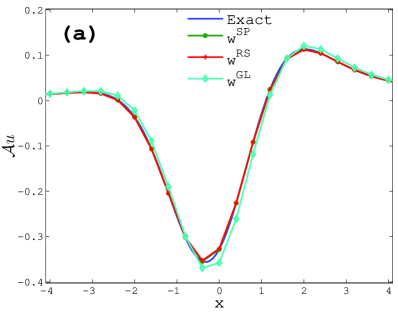
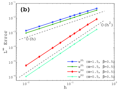
Figure 1: (a) Different approximations of $\mathcal{A}u$ for $u(x)=\frac{1}{\sqrt{2\pi}}e^{-x^{2}/2}$, and $\alpha=0.5,\beta=0.5$ with grid size $h=0.4$; (b) the convergence of the schemes with Grünwald-Letnikov weights and regularised spectral weights of the same approximations with different grid size $h$.

Different approximations to $\mathcal{A}u$ (with $\alpha=0.5,\beta=0.5$) for the Gaussian $u(x)=\frac{1}{\sqrt{2\pi}}e^{-x^{2}/2}$ on a grid size $h=0.4$ are shown in Figure 1(a), where the ’exact’ approximation is computed using high order numerical quadrature for the inverse Fourier transform. While small error could still be observed when the Grünwald-Letnikov weights are used, the approximations are almost indistinguishable from the exact value $\mathcal{A}u$ for the spectral weights and regularised spectral weights, even on a coarse grid with $h=0.4$. The above analysis about the order of accuracy is further verified in Figure 1(b), when the $L^{\infty}$ error (computed on the interval $[-4,4]$) decreases with the expected order as the grid size $h$ is refined. The spectral convergence for $w^{SP}$ is omitted in the figure, because the error is already less than $10^{-6}$ on a grid size $h=0.4$.

Notice that the above convergence rates are only expected under certain restrictions: the function $u(x)$ should be smooth enough such that the integral $\int_{|\xi|>\pi/h}\psi(-\xi)\hat{u}(\xi)e^{ix\xi}{\rm d}\xi$ can be safely ignored; care must be taken to avoid introducing any error when the infinite sum in the convolution of the scheme (10) is truncated.

4.2 Application to mean exit time

In practice, we are more interested in solutions to non-local differential equations with the generator $\mathcal{A}$, rather than approximations of the operator alone. For example, the mean exit time appears in many systems driven by various random noises [2, 6, 17]. Let the first exit time starting at $x$ from a bounded domain $\Omega$ is defined as $\tau{(\omega,x)}:=\inf\{t\geq 0,X_{0}=x,X_{t}(\omega,x)\notin\Omega\}$, and the mean first exit time (in short, mean exit time) is $u(x)=\mathbb{E}[\tau(\omega,x)].$ If $X_{t}$ is an $\alpha$-stable Lévy motion, such that $\mathbb{E}\big{(}\exp(i\xi(X_{t}-X_{0}))\big{)}=\exp(t\psi(\xi))$ with

$$\psi(\xi)=\begin{cases}-|\xi|^{\alpha}\big{(}1-i\beta\operatorname{sgn}(\xi)\tan(\alpha\pi/2)\big{)},\qquad&\alpha\neq 1,\cr-|\xi|\big{(}1-i2\beta\operatorname{sgn}(\xi)\ln|\xi|/\pi\big{)},&\alpha=1,\end{cases}$$

then the mean exit time satisfies the following nonlocal partial differential equation [5]

$$\mathcal{A}u(x) =-1,\quad\text{for}\;x\in\Omega,$$ (19)

subject to the Dirichlet-type exterior condition $u(x)\equiv 0$ for $x\in\Omega^{c}$.

Because of the zero boundary condition outside the domain, $u_{j}\equiv 0$ for $|j|\geq 1/h$ and the unknowns $\{u_{j}\}$ are governed by a linear system of equations

$$\sum_{|k|<1/h}w_{j-k}u_{k}=-1,\quad|j|<1/h.$$

This system is Toeplitz and can usually be solved very efficiently [18].

    

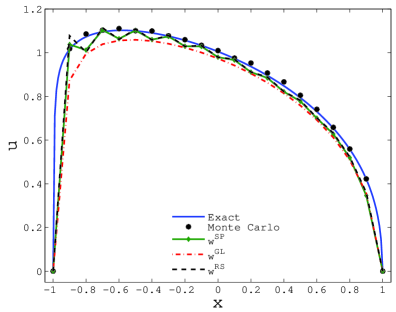
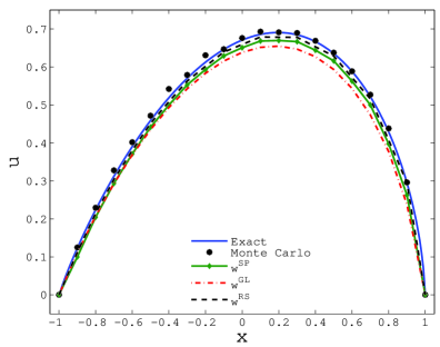
Figure 2: The solution to the mean exit problem on $\Omega=[-1,1]$, where the results from different schemes are compared with the time estimated from Monte Carlo simulations: $\alpha=0.5,\beta=0.5$ (left figure) and $\alpha=1.5,\beta=0.5$(right figure). The grid size $h$ is $0.1$ and the ’exact’ solution is obtained from the numerical solution on a refined grid $h=0.001$ using Grünwald-Letnikov weights.

The numerical solutions for $\alpha=0.5$ and $\alpha=1.5$ ($\beta=0.5$ in both cases) are show in Figure 2 with grid size $h=0.1$. As a comparison, mean exit time estimated from Monte Carlo simulation (see [16] for related random number generation) is also plotted, with 10000 sample paths for each process starting at $x$ and time step $0.0001$ for advancing the evolution. While all numerical solutions agree with the Monte Carlo simulation to some degree, new problems arise as a result of the non-smoothness of the solution $u$ near the boundaries $x=\pm 1$. For instance, the mean exit time $u(x)$ for the symmetric operator behaves like $\mbox{dist}(x,\partial\Omega)^{\alpha/2}$ near the boundary [21], which is not even Lipschitz continuous for any $\alpha\in(0,2)$. Because of this loss of regularity, the order of convergence derived in the previous subsection for each scheme no longer holds. Moreover, because of the appearance of negative weights, the numerical solutions become oscillatory, which is more pronounced when $\alpha$ is less than one, or when $|\beta|$ is close to one.

The situation is even worse for evolutionary problems when schemes with negative weights (except $w_{0}$, which is always negative yet does not affect the stability) are used—probability densities  could become negative during the evolution. In cases the underlying process is genuinely asymmetric ($\beta\neq 0$), it is common to have negative weights, because the magnitude of the integral $\int_{0}^{\pi}M_{o}(\xi)\sin(j\xi){\rm d}\xi$ usually decays to zero slower than that of $\int_{0}^{\pi}M_{e}(\xi)\cos(j\xi){\rm d}\xi$. In this regard, only the scheme with Grünwald-Letnikov weights has the desired stability property for all $\beta\in[-1,1]$.

5 Conclusion

In this paper, we proposed several difference schemes of the general form (10) for the infinitesimal generator of the $\alpha$-stable Lévy process, mainly based on the corresponding representations under the semi-discrete Fourier transform, such that the exact multiplier is properly approximated. The scheme with spectral weights $\{w_{j}^{SP}\}$ is spectrally accurate for smooth functions, but the accuracy becomes degenerate for non-smooth functions, and the solutions show spurious oscillations in the discretization of practical problems. The scheme with classical Grünwald-Letnikov weights $\{w_{j}^{GL}\}$ exhibits good numerical stability, but it is only first order accurate and a “singularity” appears when $\alpha$ approaches one. A compromise between accuracy and stability is reached in the scheme with regularised spectral weights $\{w_{j}^{RS}\}$: the accuracy is second order, adequate for most problems, while non-physical oscillations are not as pronounced as those when the spectral weights are used. The construction of high order schemes with good stability stability remains a challenging task. In practice, if the function under consideration does not decay to zero fast enough, the accuracy of the scheme could be reduced when the discrete operator $\mathcal{A}_{h}$ is just truncated to finite sums. The next order may still be recovered in many circumstances, by combining far-field asymptotic behaviour of the function and the integral representation in (2), in a similar way as in [13, Section 5]. However, this treatment of boundary condition requires certain information like the decay rate of the function that may demand deep theoretical analysis.

Appendix A The generalised hypergeometric function

The generalised hypergeometric function appears at several places in this paper, and near the origin, it is defined as a series

$${}_{p}F_{q}\big{(}a_{1},a_{2},\cdots,a_{p};b_{1},b_{2},\cdots,b_{q};z\big{)}=\sum_{n=0}^{\infty}\frac{(a_{1})_{n}(a_{2})_{n}\cdots(a_{p})_{n}}{(b_{1})_{n}(b_{2})_{n}\cdots(b_{q})_{n}n!}z^{n},$$ (20)

where $(a)_{n}=a(a+1)\cdots(a+n-1)$ is the Pochhammer symbol. The most common ones include Kummer’s confluent hypergeometric function ${}_{1}F_{1}$ and Gauss’s hypergeometric function ${}_{2}F_{1}$. From the series representation (20), it is easy to verify that

$$\frac{\mathrm{d}}{\mathrm{d}z}{}_{p}F_{q}\big{(}a_{1},a_{2},\cdots,a_{p};b_{1},b_{2},\cdots,b_{q};z\big{)}\cr=\frac{a_{1}a_{2}\cdots a_{p}}{b_{1}b_{2}\cdots b_{q}}{}_{p}F_{q}\big{(}a_{1}+1,a_{2}+1,\cdots,a_{p}+1;b_{1}+1,b_{2}+1,\cdots,b_{q}+1;z\big{)}.$$ (21)

Appendix B Special definite integrals

In the simplification of the function $\psi(\xi)$ when the Lévy measure is given by (3), the following special definite integrals are used (see [12, p.436-437]):

$$\int_{0}^{\infty}x^{-\alpha}\sin x\ \mathrm{d}x =\Gamma(1-\alpha)\cos\left(\frac{\pi\alpha}{2}\right),\qquad 0<\alpha<2$$ (22a)

$$\int_{0}^{\infty}x^{-\alpha}\cos x\ \mathrm{d}x =\Gamma(1-\alpha)\sin\left(\frac{\pi\alpha}{2}\right),\qquad 0<\alpha<1,$$ (22b)

together with other variants like

$$\int_{0}^{\infty}x^{-\alpha}(1-\cos x)\mathrm{d}x=-\Gamma(1-\alpha)\sin\left(\frac{\pi\alpha}{2}\right),\qquad 1<\alpha<3,$$ (22c)

and

$$\int_{0}^{1}\frac{\sin x-x}{x^{2}}\mathrm{d}x+\int_{1}^{\infty}\frac{\sin x}{x^{2}}\mathrm{d}x=1-\gamma,$$ (22d)

where $$\gamma$$ is the Euler-Mascheroni constant.

Appendix C Evaluation of the integrals in the weights $w^{RS}_{j}$

Here explicit expressions of the weights $\{w_{j}^{RS}\}$ associated with the regularised multipliers $M_{e}(\xi)=M_{o}(\xi)=\big{(}2-2\cos\xi)^{\alpha/2}$ are derived. In fact, $M_{e}(\xi)=M_{o}(\xi)=2^{\alpha}\sin^{\alpha}\left(\frac{\xi}{2}\right)$, and we can verify the following indefinite integral

$$\int\sin^{\alpha}\left(\frac{\xi}{2}\right)e^{ij\xi}{\rm d}\xi=\frac{i^{\alpha+1}}{2^{\alpha}(\alpha/2-j)}e^{i(j-\alpha/2)\xi}{}_{2}F_{1}\left(-\alpha,j-\frac{\alpha}{2};j+1-\frac{\alpha}{2};e^{i\xi}\right).$$ (23)

First, using (21) for the derivative of generalised hypergeometric functions, we get

$$\ \frac{e^{-i(j-\alpha/2)\xi}}{i(j-\alpha/2)}\frac{{\rm d}}{{\rm d}\xi}e^{i(j-\alpha/2)\xi}{}_{2}F_{1}\left(-\alpha,j-\frac{\alpha}{2};j+1-\frac{\alpha}{2};e^{i\xi}\right)=\cr{}_{2}F_{1}\left(-\alpha,j-\frac{\alpha}{2};j+1-\frac{\alpha}{2};e^{i\xi}\right)-\frac{\alpha e^{i\xi}}{j+1-\alpha/2}{}_{2}F_{1}\left(1-\alpha,j+1-\frac{\alpha}{2};j+2-\frac{\alpha}{2};e^{i\xi}\right).$$ (24)

By the series representation of ${}_{2}F_{1}$, the right hand side of (24) becomes

$$\quad 1+(j-\alpha/2)\sum_{n=1}^{\infty}\frac{(-\alpha)_{n}}{n!(j+n-\alpha/2)}e^{in\xi}-\alpha\sum_{n=0}^{\infty}\frac{(1-\alpha)_{n}}{n!(j+1+n-\alpha/2)}e^{i(n+1)\xi}$$

$$=1+(j-\alpha/2)\sum_{n=1}^{\infty}\frac{(-\alpha)_{n}}{n!(j+n-\alpha/2)}e^{in\xi}-\alpha\sum_{n=1}^{\infty}\frac{(1-\alpha)_{n-1}}{(n-1)!(j+n-\alpha/2)}e^{in\xi}$$

$$=1+\sum_{n=1}^{\infty}\frac{(-\alpha)_{n}}{n!}e^{in\xi},$$

which is exactly $(1-e^{i\xi})^{\alpha}$. Therefore, the indefinite integral (23) is established by

$$\quad\frac{{\rm d}}{{\rm d}\xi}\left[\frac{i^{\alpha+1}}{2^{\alpha}(\alpha/2-j)}e^{i(j-\alpha/2)\xi}{}_{2}F_{1}\left(-\alpha,j-\frac{\alpha}{2};j+1-\frac{\alpha}{2};e^{i\xi}\right)\right]\cr=\left(\frac{i}{2}\right)^{\alpha}e^{-i\alpha\xi/2}(1-e^{i\xi})^{\alpha}e^{ij\xi}=\left[\frac{e^{i\xi/2}-e^{-i\xi/2}}{2i}\right]^{\alpha}e^{ij\xi}=e^{ij\xi}\sin^{\alpha}\left(\frac{\xi}{2}\right),$$

while in the last step the principal branch of the fractional power is taken with $\xi$ assumed to be in the interval $[0,\pi]$.

Extract the real and the imaginary parts of the following integral

$$\int_{0}^{\pi}\big{(}2-2\cos\xi\big{)}^{\alpha/2}e^{ij\xi}{\rm d}\xi=\frac{i^{\alpha+1}}{\alpha/2-j}\left[e^{i(j-\alpha/2)\pi}{}_{2}F_{1}\left(-\alpha,j-\frac{\alpha}{2};j+1-\frac{\alpha}{2};-1\right)\right.\cr\left.-{}_{2}F_{1}\left(-\alpha,j-\frac{\alpha}{2};j+1-\frac{\alpha}{2};1\right)\right],$$

we get

$$\int_{0}^{\pi}\big{(}2-2\cos\xi\big{)}^{\alpha/2}\cos(j\xi){\rm d}\xi=-\frac{\Gamma(j-\alpha/2)\Gamma(1+\alpha)}{\Gamma(j+1+\alpha/2)}\sin\frac{\alpha\pi}{2},$$

and

$$\int_{0}^{\pi}\big{(}2-2\cos\xi\big{)}^{\alpha/2}\sin(j\xi){\rm d}\xi=\frac{\Gamma(j-\alpha/2)\Gamma(1+\alpha)}{\Gamma(j+1+\alpha/2)}\cos\frac{\alpha\pi}{2}\cr+\frac{(-1)^{j}}{\alpha/2-j}{}_{2}F_{1}\left(-\alpha,j-\frac{\alpha}{2};j+1-\frac{\alpha}{2};-1\right),$$

where are simplified by Gauss’s identity

$${}_{2}F_{1}\left(-\alpha,j-\frac{\alpha}{2};j+1-\frac{\alpha}{2};1\right)=\frac{\Gamma(j+1-\alpha/2)\Gamma(1+\alpha)}{\Gamma(j+1+\alpha/2)}.$$

References

- [1] D. Applebaum. Lévy processes and stochastic calculus, volume 116 of Cambridge Studies in Advanced Mathematics. Cambridge University Press, Cambridge, second edition, 2009.
- [2] Jean Bertoin. On the first exit time of a completely asymmetric stable process from a finite interval. Bull. London Math. Soc., 28(5):514–520, 1996.
- [3] K. Diethelm, N. J. Ford, A. D. Freed, and Y. Luchko. Algorithms for the fractional calculus: a selection of numerical methods. Comput. Methods Appl. Mech. Engrg., 194(6):743–773, 2005.
- [4] J. Droniou. A numerical method for fractal conservation laws. Math. Comp., 79(269):95–124, 2010.
- [5] J. Duan. An introduction to stochastic dynamics. Cambridge Texts in Applied Mathematics. Cambridge University Press, New York, 2015.
- [6] B. Dybiec, E. Gudowska-Nowak, and P. Hänggi. Lévy-brownian motion on finite intervals: Mean first passage time analysis. Phys. Rev. E, 73:046104, Apr 2006.
- [7] T. Gao, J. Duan, X. Li, and R. Song. Mean exit time and escape probability for dynamical systems driven by Lévy noises. SIAM J. Sci. Comput., 36(3):A887–A906, 2014.
- [8] R. Gorenflo, G. D. Fabritiis, and F. Mainardi. Discrete random walk models for symmetric lévy–feller diffusion processes. Physica A: Statistical Mechanics and its Applications, 269(1):79–89, 1999.
- [9] R. Gorenflo and F. Mainardi. Random walk models for space-fractional diffusion processes. Fract. Calc. Appl. Anal., 1(2):167–191, 1998.
- [10] R. Gorenflo and F. Mainardi. Random walk models approximating symmetric space-fractional diffusion processes. In Problems and methods in mathematical physics (Chemnitz, 1999), volume 121 of Oper. Theory Adv. Appl., pages 120–145. Birkhäuser, Basel, 2001.
- [11] R. Gorenflo, F. Mainardi, D. Moretti, G. Pagnini, and P. Paradisi. Discrete random walk models for space–time fractional diffusion. Chemical Physics, 284(1–2):521 – 541, 2002.
- [12] I. S. Gradshteyn and I. M. Ryzhik. Table of integrals, series, and products. Academic Press, Inc., San Diego, CA, seventh edition, 2007.
- [13] Y. Huang and A. Oberman. Numerical methods for the fractional Laplacian: a finite difference-quadrature approach. SIAM Journal on Numerical Analysis, 52(6):3056–3084, 2014.
- [14] Y. Huang and A. Oberman. Finite difference methods for fractional laplacians, 2016. preprint.
- [15] A. Iserles and S. P. Nørsett. On quadrature methods for highly oscillatory integrals and their implementation. BIT, 44(4):755–772, 2004.
- [16] A. Janicki and A. Weron. Simulation and chaotic behavior of -stable stochastic processes, volume 178 of Monographs and Textbooks in Pure and Applied Mathematics. Marcel Dekker, Inc., New York, 1994.
- [17] T. Koren, A. V. Chechkin, and J. Klafter. On the first passage time and leapover properties of Lévy motions. Phys. A, 379(1):10–22, 2007.
- [18] Michael K. Ng. Iterative methods for Toeplitz systems. Numerical Mathematics and Scientific Computation. Oxford University Press, New York, 2004.
- [19] R. H. Nochetto, E. Otárola, and A. J. Salgado. A PDE approach to fractional diffusion in general domains: a priori error analysis. Found. Comput. Math., 15(3):733–791, 2015.
- [20] K. B. Oldham and Jerome S. The fractional calculus. Academic Press [A subsidiary of Harcourt Brace Jovanovich, Publishers], New York-London, 1974.
- [21] Xavier Ros-Oton and Joaquim Serra. The dirichlet problem for the fractional laplacian: Regularity up to the boundary. Journal de Mathématiques Pures et Appliquées, 101(3):275 – 302, 2014.
- [22] S. G. Samko, A. A. Kilbas, and O. I. Marichev. Fractional integrals and derivatives. Gordon and Breach Science Publishers, Yverdon, 1993.
- [23] G. Samorodnitsky and M. S. Taqqu. Stable non-Gaussian random processes. Stochastic Modeling. Chapman & Hall, New York, 1994. Stochastic models with infinite variance.
- [24] K. Sato. Lévy processes and infinitely divisible distributions, volume 68 of Cambridge Studies in Advanced Mathematics. Cambridge University Press, Cambridge, 2013.
- [25] L. N. Trefethen. Spectral methods in MATLAB, volume 10 of Software, Environments, and Tools. Society for Industrial and Applied Mathematics (SIAM), Philadelphia, PA, 2000.
- [26] X. Wang, J. Duan, X. Li, and Y. Luan. Numerical methods for the mean exit time and escape probability of two-dimensional stochastic dynamical systems with non-Gaussian noises. Appl. Math. Comput., 258:282–295, 2015.
- [27] A. Zoia, A. Rosso, and M. Kardar. Fractional Laplacian in bounded domains. Phys. Rev. E (3), 76(2):021116, 11, 2007.