Exact solution for the force-extension relation of a semiflexible polymer under compression

Abstract

Exact solutions for the elastic and thermodynamic properties for the wormlike chain model are elaborated in terms of Mathieu functions. The smearing of the classical Euler buckling instability for clamped polymers is analyzed for the force-extension relation. Interestingly, at strong compression forces the thermal fluctuations lead to larger elongations than for the elastic rod. The susceptibility defined as the derivative of the force-extension relation displays a prominent maximum at a force that approaches the critical Euler buckling force as the persistence length is increased. We also evaluate the excess entropy and heat capacity induced by the compresssion and find that they vary non-monotonically with the load. These findings are corroborated by pseudo-Brownian simulations.

I Introduction

The elasticity of biopolymers such as actin, microtubuli, or intermediate filaments is responsible for the mechanical and structural stability of cells, their motility and intracellular transport processes Sackmann (1994); Brangwynne et al. (2006); Bausch and Kroy (2006); Fletcher and Mullins (2010); Lieleg et al. (2010); Nolting et al. (2014). Networks of these cytoskeletal polymers connected by regulatory proteins are exposed to mechanical stresses, thereby exhibiting striking nonlinear elastic behavior MacKintosh et al. (1995); Kroy and Frey (1996); Storm et al. (2005); Claessens et al. (2006); Chaudhuri et al. (2007); Huisman et al. (2008); Carrillo et al. (2013); Razbin et al. (2015); Amuasi et al. (2015); Plagge et al. (2016). An adequate characterization of the mechanical properties of these biological assemblies constitutes a fundamental step toward the future design and synthesis of artificial biomimetic materials Ratner et al. (2004); Ratner and Bryant (2004). Since the macroscopic behavior of these filamentous materials strongly depends on the properties of their constituents, a profound knowledge on the nature of single filaments is necessary to fully understand the elasticity of these networks Hugel and Seitz (2001).

Due to their semiflexibility, biopolymers show a peculiar response to external forces Ott et al. (1993); Broedersz and MacKintosh (2014); Razbin et al. (2016), where the static and dynamic properties are dominated by their enthalpic elasticity, but conformational entropy still plays a significant role. Experimental techniques such as optical Ashkin (1997); Mehta et al. (1999) and magnetic tweezers Gosse and Croquette (2002), transmission electron microscopy Kuzumaki and Mitsuda (2006), and (atomic) force spectroscopy Janshoff et al. (2000); Hugel and Seitz (2001) have been used to quantify the mechanical properties in terms of force-extension relations Saleh (2015). These capture the nonlinear effects emerging in the stretching and buckling of semiflexible polymers such as DNA Marko and Siggia (1995); Bouchiat et al. (1999); Bustamante et al. (2000), actin Liu and Pollack (2002), and synthetic carbon nanotubes Kuzumaki and Mitsuda (2006), but also single molecules such as titin Kellermayer et al. (1997), which is an important component in striated muscle tissues, and collagen Sun et al. (2002), present in, e.g., skin and bones.

To characterize theoretically the physics of the nonlinear elastic behavior of semiflexible polymers, the wormlike chain (WLC), also referred to as Kratky-Porod model Kratky and Porod (1949) has been analyzed in terms of the end-to-end distribution function in the weakly-bending approximation  Wilhelm and Frey (1996) as well as in terms of the exact low-order moments Hamprecht et al. (2004); Spakowitz et al. (2004); Spakowitz and Wang (2005); Mehraeen et al. (2008). The WLC model has been shown to be a reliable model for semiflexible polymers, as it reproduces, e.g., the mechanical behavior of DNA Marko and Siggia (1995) and actin Liu and Pollack (2002), while for microtubuli internal shearing of adjacent protofilaments leads to an apparent length dependence of the elastic moduli Taute et al. (2008); Pampaloni et al. (2006). In these studies, approximate solutions of the force-extension relation of stretched polymers have been compared to experimental data in order to determine mechanical properties such as the persistence length.

The approximations have been complemented by exact expressions for stretched polymers in the plane Prasad et al. (2005), while force-extension relations of polymers under a compressive load have so far only been analyzed within the regime of stiff polymers Baczynski et al. (2007); Emanuel et al. (2007); Lee et al. (2007); Bedi and Mao (2015). Therefore, a characterization of the buckling behavior for a broad range of semiflexible polymers is needed to predict elastic properties within experimental observations.

Here, we provide an exact analytical solution for the force-extension relation of a compressed semiflexible polymer within the framework of the WLC model and compare the results for polymers with different rigidity to computer simulations. Boundary conditions imposed within the experimental setup play a crucial role for the response of polymers to external forces, as has been discussed earlier for stretched polymers Ghosh et al. (2007). To quantify this effect, we also compare the force-extension relations with two clamped ends, one free and one clamped end, and two free ends. Thermodynamic properties, such as the in principle measurable excess heat capacity of the semiflexible polymers induced by the compression, are also discussed.

II The wormlike chain model

For the elastic properties of a semiflexible polymer, we rely on the WLC model Kratky and Porod (1949), where the bending energy of an inextensible semiflexible polymer is expressed by its squared curvature,

$$\mathcal{H}_{0} =\frac{\kappa}{2}\int_{0}^{L}\mathrm{d}s\ \Bigl{(}\frac{\mathrm{d}\mathbf{u}(s)}{\mathrm{d}s}\Bigr{)}^{2}.$$ (1)

Here, $s$ is the arc length, $\mathbf{u}(s)=\mathrm{d}\mathbf{r}(s)/\mathrm{d}s$ denotes the tangent vector of the polymer along its contour $\mathbf{r}(s)$, $\kappa$ the bending stiffness of the polymer, and $L$ its contour length. The corresponding partition sum $Z_{0}(\mathbf{u}_{L},L|\mathbf{u}_{0},0)$ of the polymer with initial orientation $\mathbf{u}_{0}$ and final orientation $\mathbf{u}_{L}$ is obtained as a sum of Boltzmann weights over all possible configurations,

$$Z_{0}(\mathbf{u}_{L},L|\mathbf{u}_{0},0) =\int_{\mathbf{u}(0)=\mathbf{u}_{0}}^{\mathbf{u}(L)=\mathbf{u}_{L}}\mathcal{D}[\mathbf{u}(s)]\exp(-\mathcal{H}_{0}/k_{\text{B}}T),$$ (2)

where the inextensibility constraint $|\mathbf{u}(s)|=1$ has to be fulfilled. In addition, if the polymer is subject to a constant external force $\mathbf{F}$, the stretching energy,

$$\mathcal{H}_{\text{force}} =-\int_{0}^{L}\mathrm{d}s\ \mathbf{F}\cdot\mathbf{u}(s),$$ (3)

has to be added to the bending energy. Here, the force acts along a fixed direction $\mathbf{e}$ with strength $F$ such that $\mathbf{F}=F\mathbf{e}$. Collecting terms, the full Hamiltonian of the system reads

$$\frac{\mathcal{H}}{k_{\text{B}}T} =\int_{0}^{L}\mathrm{d}s\ \Bigl{[}\frac{\kappa}{2k_{\text{B}}T}\Bigl{(}\frac{\mathrm{d}\mathbf{u}(s)}{\mathrm{d}s}\Bigr{)}^{2}-f\mathbf{e}\cdot\mathbf{u}(s)\Bigr{]},$$ (4)

where $f=F/k_{\text{B}}T$ is the reduced force with units of an inverse length. The persistence length $\ell_{\text{p}}=\kappa/k_{\text{B}}T$ for 3D, respectively $\ell_{\text{p}}=2\kappa/k_{\text{B}}T$ for 2D, corresponds to the decay length of the tangent-tangent correlations of the polymer and permits a classification of polymers into three categories: polymers with $\ell_{\text{p}}/L\ll 1$ are referred to as flexible and therefore more coil-like structured, $\ell_{\text{p}}/L\sim 1$ are semiflexible, and $\ell_{\text{p}}/L\gg 1$ are stiff, hence, rodlike Doi and Edwards (1986); Broedersz and MacKintosh (2014). The partition sum $Z(\mathbf{u}_{L},L|\mathbf{u}_{0},0)$ of such a polymer subject to an external force is given by the path integral over all weighted, accessible chain configurations. In particular, except for the prefactor $Z_{0}\equiv Z_{0}(\mathbf{u}_{L},L|\mathbf{u}_{0},0)$, the partition sum can be viewed as the generating function of a semiflexible polymer:

$$Z(\mathbf{u}_{L},L|\mathbf{u}_{0},0) =\int_{\mathbf{u}(0)=\mathbf{u}_{0}}^{\mathbf{u}(L)=\mathbf{u}_{L}}\mathcal{D}[\mathbf{u}(s)]\exp(-\mathcal{H}/k_{\text{B}}T),$$ (5)

$$=Z_{0}\left\langle\exp\left(\int_{0}^{L}\mathrm{d}sf\mathbf{e}\cdot\mathbf{u}\right)\right\rangle.$$ (6)

The corresponding thermodynamic potential is the Gibbs free energy defined by

$$G(T,F) =-k_{\text{B}}T\ln[Z(\mathbf{u}_{L},L|\mathbf{u}_{0},0)],$$ (7)

with fundamental relation

$$\mathrm{d}G =-S\mathrm{d}T-\langle X\rangle\mathrm{d}F,$$ (8)

where $S=S(T,F)$ denotes the entropy of the polymer and $\langle X\rangle:=\int_{0}^{L}\mathrm{d}s\ \langle\mathbf{e}\cdot\mathbf{u}(s)\rangle$ is the mean end-to-end distance projected onto the direction of the force.

Hence, the mean projected end-to-end distance is obtained by

$$\langle X\rangle =-\left(\frac{\partial G}{\partial F}\right)_{T}=-\frac{1}{k_{\text{B}}T}\left(\frac{\partial G}{\partial f}\right)_{T}.$$ (9)

In particular, the response of the polymer to the applied force is encoded in the isothermal susceptibility,

$$\chi =\left(\frac{\partial\langle X\rangle}{\partial F}\right)_{T}=\frac{1}{k_{\text{B}}T}\left(\frac{\partial\langle X\rangle}{\partial f}\right)_{T},$$ (10)

which characterizes the strength of the response with respect to the applied force. Furthermore it serves as an indicator for the buckling force of semiflexible polymers in analogy to the critical Euler buckling force for stiff rods Landau and Lifshitz (1986).

We can also obtain the linear susceptibility $\chi$ in terms of the fluctuation-response theorem Doi and Edwards (1986) for the semiflexible polymer,

$$\chi(T,F) =\frac{1}{k_{\text{B}}T}\left\langle\left(X-\langle X\rangle\right)^{2}\right\rangle.$$ (11)

In addition to these elastic properties, we obtain the change in the entropy with respect to the force at constant temperature by using the Maxwell relation:

$$\left(\frac{\partial S}{\partial F}\right)_{T} =\left(\frac{\partial\langle X\rangle}{\partial T}\right)_{F}.$$ (12)

Thus, the excess entropy $\Delta S(T,F)=S(T,F)-S(T,F=0)$ can then be evaluated by

$$\Delta S(T,F) =\int_{0}^{F}\mathrm{d}F^{\prime}\left(\frac{\partial\langle X\rangle}{\partial T}\right)_{F^{\prime}}.$$ (13)

Similarly, the experimentally accessible excess heat capacity $\Delta C_{F}(T,F)=C_{F}(T,F)-C_{F}(T,F=0)$ is obtained by

$$\Delta C_{F}(T,F) =\int_{0}^{F}\mathrm{d}F^{\prime}\ T\left(\frac{\partial^{2}\langle X\rangle}{\partial T^{2}}\right)_{F^{\prime}}.$$ (14)

II.1 Analytic solution

To determine the elastic and thermodynamic properties, the partition sum has to be computed by solving for the path integral [Eq. (5)]. Therefore, we discretize the path integral in terms of the arc-length Kleinert (2009) and find that the partition sum obeys an equation of the Schrödinger type, describing the evolution of the partition sum along the contour of the polymer,

$$\partial_{s}Z(\mathbf{u},s|\mathbf{u}_{0},0) =[f\mathbf{e}\cdot\mathbf{u}+\frac{k_{\text{B}}T}{2\kappa}\Delta_{\mathbf{u}}]Z(\mathbf{u},s|\mathbf{u}_{0},0),$$ (15)

where $\Delta_{\mathbf{u}}$ denotes the angular part of the Laplacian, and with initial condition

$$Z(\mathbf{u},s=0|\mathbf{u}_{0},0) =\delta(\mathbf{u},\mathbf{u_{0}}),$$ (16)

such that the delta function $\delta(\cdot,\cdot)$ enforces both orientations to coincide.

Here we restrict the discussion to a polymer confined to a plane. Consequently, the inextensibility constraint of the orientation can be parametrized in terms of a polar angle, $\mathbf{u}=(\cos\varphi,\sin\varphi)^{T}$, were the angle $\varphi$ is measured with respect to the direction of the applied force. Thus, the evolution of the partition sum along the arc length reads

$$\partial_{s}Z(\varphi,s|\varphi_{0},0) =\left[f\cos(\varphi)+\frac{1}{\ell_{\text{p}}}\partial^{2}_{\varphi}\right]Z(\varphi,s|\varphi_{0},0),$$ (17)

subject to the initial condition

$$Z(\varphi,s=0|\varphi_{0},0) =\delta(\varphi-\varphi_{0}\text{ mod }2\pi).$$ (18)

The Fokker-Planck equation [Eq. (17)] is reminiscent of the Schrödinger equation of a quantum pendulum Aldrovandi and Ferreira (1980) and can be solved analytically by separation of variables in terms of appropriate angular eigenfunctions, $\exp(-\lambda s)z(\varphi)$. Inserting this ansatz into Eq. (17), we obtain

$$\left[\lambda+f\cos\varphi+\frac{1}{\ell_{\text{p}}}\frac{\mathrm{d}^{2}}{\mathrm{d}\varphi^{2}}\right]z(\varphi) =0.$$ (19)

Here we focus on a polymer exposed to a compressive load, in particular, we rewrite the reduced force as $f=-|f|$. A change of variables $x=\varphi/2$ and rearranging terms, leads to the equation

$$\left[\frac{\mathrm{d}^{2}}{\mathrm{d}x^{2}}+\left(a-2q\cos(2x)\right)\right]z(x)=0,$$ (20)

which is known as the Mathieu equation DLMF ; Olver et al. (2010) with deformation parameter $q=2|f|\ell_{\text{p}}$ and eigenvalue $a=4\ell_{\text{p}}\lambda$. Thus, the general solution is expressed as a linear combination of $\pi$-periodic even and odd Mathieu functions $\text{ce}_{2n}(q,x)$ and $\text{se}_{2n+2}(q,x)$ with corresponding eigenvalues $a_{2n}\equiv a_{2n}(q)=4\ell_{\text{p}}\lambda_{n}$ and $b_{2n+2}\equiv b_{2n+2}(q)=4\ell_{\text{p}}\lambda_{n}$ DLMF ; Olver et al. (2010), respectively. Note that in the case of a polymer under tension, where the sign of the force is positive, $f=|f|$, a different change of variables $x=\pi/2-\varphi/2$ has to be used in order to arrive at the Mathieu equation Prasad et al. (2005).

The Mathieu functions are essentially deformed sines and cosines:

$$\text{ce}_{2n}(q,x) =\sum_{m=0}^{\infty}A_{2m}^{2n}(q)\cos(2mx),$$ (21)

$$\text{se}_{2n+2}(q,x) =\sum_{m=0}^{\infty}B_{2m+2}^{2n+2}(q)\sin\bigl{(}(2m+2)x\bigr{)}.$$ (22)

The coefficients $A_{2m}^{2n}(q)$ and $B_{2m+2}^{2n+2}(q)$ are determined by recurrence relations, which result from inserting the Fourier series into Eq. (20):

$$a_{2n}A_{0}^{2n}-qA_{2}^{2n} =0,$$ (23)

$$(a_{2n}-4)A_{2}^{2n}-q(2A_{0}^{2n}+A_{4}^{2n}) =0,$$ (24)

$$(a_{2n}-4m^{2})A_{2m}^{2n}-q(A_{2m-2}^{2n}+A_{2m+2}^{2n}) =0,\quad m\geq 2,$$ (25)

and similar relations hold for the coefficients $B_{2m+2}^{2n+2}(q)$ DLMF ; Olver et al. (2010). The Mathieu functions constitute a complete, orthogonal and normalized set of eigenfunctions: $\int_{0}^{2\pi}\mathrm{d}x\ \text{ce}_{2n}(q,x)\text{ce}_{2m}(q,x)=\delta_{nm}\pi$ and similarly for $\text{se}_{2n+2}(q,x)$. Hence, the full solution of Eq. (17) in terms of the eigenfunctions reads

$$Z(\varphi_{L},L|\varphi_{0},0)=$$

$$\frac{1}{2\pi}\sum_{n=0}^{\infty}\bigl{[}\text{ce}_{2n}(q,\varphi_{0}/2)\text{ce}_{2n}(q,\varphi_{L}/2)e^{-a_{2n}(q)L/4\ell_{\text{p}}}$$

$$+\text{se}_{2n+2}(q,\varphi_{0}/2)\text{se}_{2n+2}(q,\varphi_{L}/2)e^{-b_{2n+2}(q)L/4\ell_{\text{p}}}\bigr{]}.$$ (26)

Since the eigenvalues are ordered with increasing $n$, $a_{0}(q)<b_{2}(q)<a_{2}(q)<b_{4}(q)<...$, the series expansion converges and can be evaluated numerically, which is discussed in more detail in Appendix A.

We impose boundary conditions, that reflect different experimental setups accounting for clamped or free orientations at the ends of the polymer. The presented partition sum [Eq. (26)] represents the case of a clamped polymer with given initial and final orientation. This can be complemented by two or more scenarios. First, we look at a half-clamped polymer, where the initial orientation is clamped and the final one is free. The corresponding partition sum $Z(L|\varphi,0)$ is obtained via integration over all final angles,

$$Z(L|\varphi_{0},0)=\int_{0}^{2\pi}\mathrm{d}\varphi_{L}Z(\varphi_{L},L|\varphi_{0},0),$$

$$=\sum_{n=0}^{\infty}A_{0}^{2n}(q)\text{ce}_{2n}(q,\varphi_{0}/2)\exp[-a_{2n}(q)L/4\ell_{\text{p}}],$$ (27)

where $A_{0}^{2n}(q)$ results from the integral over the even Mathieu functions and the odd Mathieu functions do not contribute anymore.

Further, integrating also over the initial angle the partition sum corresponding to a free polymer reduces to

$$Z(L) =2\pi\sum_{n=0}^{\infty}[A_{0}^{2n}(q)]^{2}\exp[-a_{2n}(q)L/4\ell_{\text{p}}].$$ (28)

Interestingly, the same result occurs for the semiflexible polymer under tension Prasad et al. (2005), which reflects that the polymer is free to align with the external force. To evaluate the partition sums in Eqs. (26) and (27) numerically, we rely on an implementation of the Mathieu functions in a computer algebra system Wolfram Research (2016). However, to determine the Fourier coefficients $A_{0}^{2n}(q)$ in Eqs. (27) and (28) it is more efficient to solve numerically the eigenvalue problem of the recurrence relations [Eq. (23)-(25)].

II.2 Linear response

The linear response $\chi(T,F=0)$ of the semiflexible polymer to the compression force can also be obtained exactly by expanding the full solution in Eqs. (26), (27), and (28) to second order in the force. For a clamped polymer we use the expansions of the Mathieu functions for $\varphi_{0}=\varphi_{L}=0$ and the corresponding eigenvalues up to second order in the deformation parameter $q$ from Refs. DLMF ; Olver et al. (2010):

$$a_{0}(q) =-\frac{q^{2}}{2},\ a_{2}(q)=4+\frac{5q^{2}}{12},$$ (29)

$$a_{2n}(q) =4n^{2}+\frac{q^{2}}{2(4n^{2}-1)},$$ (30)

$$\text{ce}_{0}(q,0) =\frac{1}{\sqrt{2}}\left(1-\frac{q}{2}-\frac{q^{2}}{32}\right),$$ (31)

$$\text{ce}_{2}(q,0) =1+\frac{q}{6}-\frac{73q^{2}}{1152},$$ (32)

$$\text{ce}_{2n}(q,0) =1-\frac{q}{2-8n^{2}}+\frac{(8n^{2}+1)q^{2}}{32\left(1-4n^{2}\right)^{2}\left(n^{2}-1\right)}.$$ (33)

Note that for $\varphi_{0}=\varphi_{L}=0$ the odd Mathieu functions do not contribute to the partition sum. Inserting these expansions into the full solution [Eq. (26)] one can derive both the projected mean end-to-end distance as well as the force-free susceptibility [Eq. (11)]. The explicit expressions are rather lengthy for arbitrary parameters $L$ and $\ell_{\text{p}}$ and will not be shown here, but we will discuss them for a clamped polymer in Sec. III, Fig. 3.

For the half-clamped polymer ($\varphi_{0}=0$) only the first three terms, $n=0,1,2,$ contribute to the order considered to the partition sum in Eq. (27). Here, we use the expansions up to second order in $q$ of the Fourier coefficients $A_{0}^{0}(q)=(1-q^{2}/16)/\sqrt{2}$, $A_{0}^{2}(q)=q/4$ and $A_{0}^{4}(q)=q^{2}/96$ obtained from Refs. DLMF ; Olver et al. (2010), and inserted these together with the expansions from Eqs.(29)-(33) into the full solution [Eq. (27)]. Thus, the partition sum reads

$$Z (L|\varphi_{0}=0,0)=\pi+\pi\ell_{\text{p}}\frac{|F|}{k_{\text{B}}T}\left(e^{-L/\ell_{\text{p}}}-1\right)$$

$$+\frac{\pi}{24}\ell_{\text{p}}^{2}\left(\frac{|F|}{k_{\text{B}}T}\right)^{2}\Bigl{(}\frac{12L}{\ell_{\text{p}}}-9+8e^{-L/\ell_{\text{p}}}+e^{-4L/\ell_{\text{p}}}\Bigr{)}$$

$$+\mathcal{O}\left(|F|^{3}\right),$$ (34)

which results in a projected mean end-to-end distance

$$\langle X\rangle =\left(\ell_{\text{p}}-\ell_{\text{p}}e^{-L/\ell_{\text{p}}}\right)+\frac{\ell_{\text{p}}|F|}{12k_{\text{B}}T}\Bigl{\{}\ell_{\text{p}}\Bigl{[}e^{-4L/\ell}\Bigl{(}12e^{2L/\ell}$$

$$\ \ \ -32e^{3L/\ell}-1\Bigr{)}+21\Bigr{]}-12L\Bigr{\}}+\mathcal{O}\left(|F|^{2}\right),$$ (35)

and linear susceptibility

$$\chi(T,F=0) =\frac{\ell_{\text{p}}}{12k_{\text{B}}T}\Bigl{[}\ell_{\text{p}}\Bigl{(}e^{-4L/\ell_{\text{p}}}-12e^{-2L/\ell_{\text{p}}}$$

$$\ \ \ +32e^{-L/\ell_{\text{p}}}-21\Bigr{)}+12L\Bigr{]}.$$ (36)

For the free polymer only the first two terms contribute and the partition sum in Eq. (28) is evaluated similar to the partition sum of a half-clamped polymer [Eq. (34)]. It reduces to

$$Z(L) =\pi^{2}+\frac{\pi^{2}}{2}\ell_{\text{p}}^{2}\left(\frac{|F|}{k_{\text{B}}T}\right)^{2}\left(e^{-L/\ell_{\text{p}}}+\frac{L}{\ell_{\text{p}}}-1\right)+\mathcal{O}\left(|F|^{3}\right).$$ (37)

Here the projected mean end-to-end distance vanishes for zero force after averaging over the initial and final angles,

$$\langle X\rangle =\frac{\ell_{\text{p}}|F|}{k_{\text{B}}T}\left[\ell_{\text{p}}\left(1-e^{-L/\ell_{\text{p}}}\right)-L\right]+\mathcal{O}\left(|F|^{2}\right),$$ (38)

and the linear susceptibility reads

$$\chi(T,F=0) =\frac{\ell_{\text{p}}}{k_{\text{B}}T}\left[\ell_{\text{p}}\left(e^{-L/\ell_{\text{p}}}-1\right)+L\right].$$ (39)

II.3 Pseudodynamics

To validate our analytical results, we also simulate the semiflexible polymer under compression. To generate a set of representative conformations of the polymer in equilibrium, we rely on Brownian dynamics simulations that yield the canonical ensemble as stationary state. Since we are not interested in the dynamic properties here, features such as hydrodynamic interactions, anisotropic friction, and the overall translational motion are ignored. Thus the purpose of the pseudodynamics is merely to reproduce the equilibrium properties.

We first discretize equidistantly the contour $L$ of the polymer in terms of the positions of the beads $\{\mathbf{R}_{i}\}_{i=0}^{N}$ and corresponding tangent vectors $\{\mathbf{u}_{i}\}_{i=0}^{N-1}$, where $\mathbf{u}_{i}=(\mathbf{R}_{i+1}-\mathbf{R}_{i})N/L$ is of unit length, $|\mathbf{u}_{i}|=1$.

The pseudodynamics for the orientation of the $i$th bead is prescribed by the Langevin equation in the It$\bar{\text{o}}$ sense,

$$\mathrm{d} \mathbf{u}_{i}(t)=-\hat{D}_{\text{rot}}\mathbf{u}_{i}(t)\mathrm{d}t+\hat{D}_{\text{rot}}\mathbf{u}_{i}^{\perp}(t)\Bigl{(}\frac{N}{L}\frac{\ell_{\text{p}}}{2}\mathbf{u}_{i}^{\perp}(t)\cdot[\mathbf{u}_{i-1}(t)$$

$$+\mathbf{u}_{i+1}(t)]-\frac{L}{N}|f|\mathbf{u}^{\perp}_{i}(t)\cdot\mathbf{e}\Bigr{)}\mathrm{d}t+\sqrt{2\hat{D}_{\text{rot}}}\mathbf{u}_{i}^{\perp}(t)\mathrm{d}\omega_{i}(t),$$ (40)

for $i=1,\dotsc,N-2$ and appropriately modified Langevin equations at the boundary, $i=0,N-1$. Here $\mathbf{u}_{i}^{\perp}(t)$ is the unit orientation rotated clockwise by an angle of $\pi/2$, i.e. $\mathbf{u}_{i}^{\perp}(t)\cdot\mathbf{u}_{i}(t)=0$ and $\det[\left(\mathbf{u}_{i}(t),\mathbf{u}_{i}^{\perp}(t)\right)]=1$. Furthermore $\omega_{i}(t)$ is a Gaussian white noise process with zero mean and variance $\langle\omega_{i}(t)\omega_{j}(t^{\prime})\rangle=\delta_{ij}\delta(t-t^{\prime})$ for $i,j=0,\dotsc,N-1$. The scaled rotational diffusion of the orientations $\hat{D}_{\text{rot}}$ sets only the time scale in our case. We show in Appendix B that the Langevin equations [Eq. (40)] in fact reproduce the canonical ensemble of the semiflexible polymer problem.

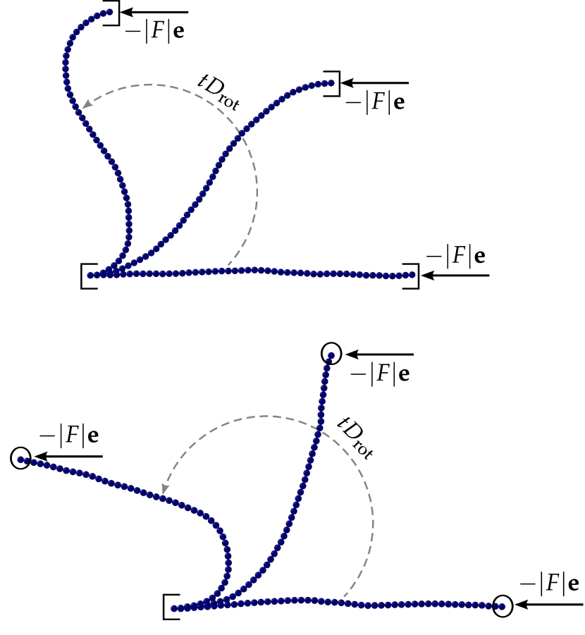
Figure 1: Typical time evolution in simulation of a clamped (top) and a half-clamped (bottom) polymer starting from a straight configuration. The simulation is for a rather stiff polymer, $\ell_{\text{p}}=10L$, subject to a strong compression force $|F|=2F_{c}$.

The boundary conditions for a clamped polymer are set by fixed initial and final orientation chosen into the direction antiparallel to the compression force, in particular, $\mathbf{u}_{0}(t)=\mathbf{u}_{N-1}(t)=-\mathbf{e}$ for all times $t$. A half-clamped polymer fulfills the same boundary condition for the initial orientation, $\mathbf{u}_{0}(t)=-\mathbf{e}$, whereas the final orientation can freely rotate.

Simulation snapshots [Fig. 1] reveal that a semiflexible polymer shows qualitatively different buckling behavior with respect to the boundary conditions. Since clamped polymers cannot rotate their ends, they exhibit an S-shaped configuration under a compressive load. In contrast, if the second end of the polymer is free to rotate, it can align with the direction of the applied force and a hook-shape configuration is observed. Considering two free ends the polymer will just rotate under the force and thus its behavior is expected to be identical to that of a polymer under tension.

To obtain reliable statistics in equilibrated configurations we have conducted $120$ realizations of a polymer with $N=300$ segments and a time step of $10^{-5}/\hat{D}_{\text{rot}}$ over a time horizon of $10^{3}/\hat{D}_{\text{rot}}$. Measurements are taken after the polymer has reached equilibrium. For a free polymer the simulations have been performed over a longer time horizon of $10^{4}/\hat{D}_{\text{rot}}$, however, with fewer realizations, since the free rotation of the polymer requires long transients to reach equilibrium at low forces.

In addition we have performed Monte Carlo simulations, similar to Ref. Baczynski et al. (2007), to crosscheck the results. They confirm our analytical predictions for clamped polymers, but they start to fail in terms of convergence and statistics when refining the discretization to capture the semiflexibility of the polymers and also the simulation of a free polymer has been demanding.

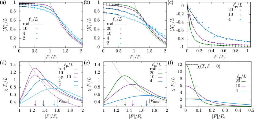
Figure 2: End-to-end distance in the direction of the applied force (top) and susceptibility (bottom) of polymers with different persistence lengths and boundary conditions, clamped (a) and (d), half-clamped (b) and (e), and free ends (c) and (f). The black dashed lines indicate the linear response and the gray dashed line corresponds to the classical Euler buckling, $F_{c}$ is the classical Euler buckling force $F_{c}=\pi^{2}\kappa/(\gamma L)^{2}$. In (c) and (f) we use $\gamma=2$ in $F_{c}$ to normalize the forces. The forces $|F_{\text{max}}|$ are extracted from the maxima of the susceptibility. In Fig. (d) the dashed line (ap. 10) represents the approximate susceptibility derived from the solution in Ref. Baczynski et al. (2007). Theory and pseudodynamics simulations are shown with lines and dots, respectively.

II.4 Classical Euler buckling

A stiff rod under compression at small forces does not yield at all but starts to buckle at a critical force that is known as the Euler buckling instability Landau and Lifshitz (1986). The critical force is determined by the rigidity $\kappa$ and the contour length $L$ by

$$F_{c} =\frac{\pi^{2}\kappa}{(\gamma L)^{2}},$$ (41)

where $\gamma$ accounts for the different boundary conditions. In the case of a clamped rod, $\gamma=1$, with one end fixed and one translationally free; however, if one end of the rod is clamped and one orientationally and translationally free, $\gamma=2$ Landau and Lifshitz (1986).

For small temperatures the Fokker-Planck equation [Eq. (17)] of the partition sum can be approximated for a stiff rod by an Eikonal approximation Kleinert (2009). Here we set the partition sum $Z=\exp(-G/k_{\text{B}}T)$, neglect terms of higher order in the inverse temperature, and consequently obtain the approximate equation for the Gibbs free energy,

$$\partial_{s}G-|F|\cos\varphi\ G+\frac{1}{2\kappa}\left(\partial_{\varphi}G\right)^{2} =0.$$ (42)

Using the method of characteristics leads to the equation of motion for the angle,

$$\kappa\frac{\mathrm{d}^{2}\varphi(s)}{\mathrm{d}s^{2}}+|F|\sin\varphi(s) =0,$$ (43)

which is as anticipated reminiscent of the equation of motion of a classical pendulum Aldrovandi and Ferreira (1980). The same equation results as Euler-Lagrange equation minimizing the total energy [Eq. (4)]. Starting from this equation, the force-extension relation for $|F|>F_{c}$ of a clamped and half-clamped rod is well known Landau and Lifshitz (1986); Baczynski et al. (2007),

$$\langle X\rangle =\sqrt{\frac{2\kappa}{|F|}}\int_{0}^{\varphi_{L/2}}\mathrm{d}\varphi\ \frac{\cos\varphi}{\sqrt{\cos\varphi-\cos\varphi_{L/2}}}.$$ (44)

These results will be compared to the elastic properties of semiflexible polymers confined to two dimensions.

III Elastic properties

In this section we provide a discussion of the analytic solution and simulation results for the force-extension relation and the associated susceptibility.

Clamped polymer: The mean projected end-to-end distance $\langle X\rangle$ of a clamped polymer is obtained by numerical differentiation of the Gibbs free energy [Eq. (9)]. We find a smooth monotone crossover from an almost stretched to a buckled configuration with increasing compression force, in contrast to the classical Euler buckling instability, where the first yielding takes place at the critical force $F_{c}$ [Fig. 2 (a)]. Due to thermal fluctuations already for vanishing forces, semiflexible polymers display undulations, hence, their projected end-to-end distance is shorter than their contour length, $\langle X\rangle<L$. As anticipated, in the regime of small forces higher flexibility leads to shorter mean end-to-end distances, which approach zero for completely flexible polymers, $\ell_{\text{p}}/L\ll 1$. Qualitatively, the linear response behavior appears to be correct up to forces comparable to the classical Euler buckling force (see Figs. 2  (a) and (b)). Interestingly, for increasing forces, $|F|>F_{c}$, the end-to-end distance of semiflexible polymers intersects with that of a stiff rod, indicating a stiffening of the polymer due to thermal fluctuations. A similar trend occurs when comparing different persistence lengths, hence, initially more flexible polymers yield more strongly while for large forces they resist harder than stiffer polymers.

Furthermore we compare the susceptibility $\chi$ of semiflexible polymers in response to the compression force to the susceptibility of a stiff rod [Fig. 2 (d)]. The latter vanishes for forces smaller than the critical Euler buckling force, reflecting that a classical rod does not yield. Directly at the transition the classical susceptibility assumes the value $\chi(F_{c}+0)=2L/F_{c}$ and decreases monotonically for larger forces. In contrast the susceptibility of semiflexible polymers initially increases starting from $\chi(T,F=0)$ as predicted from the linear response (not shown), then displays a maximum at a force $|F_{\text{max}}|$, which exceeds the Euler buckling force, $|F_{\text{max}}|>F_{c}$. Increasing the stiffness, this force approaches the critical buckling force $|F_{\text{max}}|\downarrow F_{c}$, which suggests to use $|F_{\text{max}}|$ as a measure to charactzerize the smooth transition for fluctuating semiflexible polymers. For simplicity, we refer to $|F_{\text{max}}|$ as the buckling force also in the case of non-zero temperature. Interestingly, for stronger forces the projected end-to-end distance becomes even negative (see Fig. 3), which reflects the S-shaped configuration in Fig. 1.

Half-clamped polymer: Here, the force-extension relation behaves similarly to the one for clamped polymers (see Fig. 2 (b)). Nevertheless half-clamped polymers yield more strongly even after taking into account that the classical buckling force is reduced by a factor of $\gamma^{2}=4$ due to the different boundary conditions. In fact, the data demonstrate that the semiflexibility becomes more important for half-clamped polymers.

Qualitatively, the monotonous transition from the straightened to the buckled configuration of these polymers remains unchanged, intersections with the end-to-end distance of a stiff rod persist also here. The corresponding susceptibilities [Fig. 2 (e)] are less pronounced in comparison to clamped polymers of the same stiffness [Fig. 2 (d)]. Also, here we characterize the transition by a buckling force $|F_{\text{max}}|$ taken as the maximum of the susceptibility. For half-clamped ends the approach $|F_{\text{max}}|\downarrow F_{c}$ is slower than for clamped ends.

Free polymer: In contrast to clamped polymers, the force-extension relation of a free polymer exhibits qualitatively different behavior (see Fig. 2 (c)). Direct inspection of the configurations (not shown) reveals that the polymer essentially rotates and aligns with the direction of the force. Thus, rather than compressing, the force in fact stretches the polymer in the reverse direction, in particular, the projected end-to-end distances are all negative. The analytic solution for the case of pulling has been provided before Prasad et al. (2005), however, only an approximate solution for rather flexible polymers of length $L>4\ell_{\text{p}}$ has been discussed in more detail. Thermal undulations prevent the polymer to be in a completely straight configuration. Stiffer polymers react to smaller forces than more flexible polymers, and extend nearly to their full contour length. For free ends the force-extension relations approach monotonically the case of a fully aligned rod as the stiffness increases, in contrast to the other two boundary conditions. Similarly, the susceptibility [Fig. 2 (f)], is always maximal at vanishing forces, where it assumes the value $\chi(T,F=0)$ as predicted by linear response theory, and is larger for increasing stiffness. Correspondingly, no characteristic buckling force is extracted for this case, since after all the polymer stretches rather than buckles in this case.

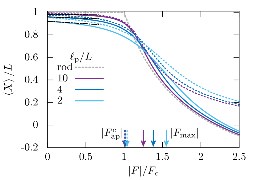
Figure 3: Comparison of our analytic results to the approximate solution (dashed lines) of Ref. Baczynski et al. (2007) for different persistence lengths. $|F_{\text{max}}|$ denotes the force at maximal susceptibility from the analytic theory and $|F_{\text{ap}}^{c}|$ the critical force for the onset of buckling, taken from Ref. Baczynski et al. (2007). The black dashed line indicates the linear response, and the gray dashed line corresponds to the classical Euler buckling.

Approximate Solution: An approximate solution of the force-extension relation in the regime of rather stiff polymers has been presented by Baczynski et al. Baczynski et al. (2007) by integrating out short wavelength fluctuations. Their results predict qualitatively similar behavior for clamped polymers in terms of the smooth buckling transition. Yet, already in the regime for small forces $|F|\lesssim F_{c}$ deviations to our analytic theory become apparent (see Fig. 3). The differences decrease as stiffer polymers are considered. Their approximate solution for stiff polymers exhibits far weaker buckling than the predicted analytic solution and in addition the force-extension relation remains positive for all forces. This finding is not in agreement with the analytic solution for semiflexible polymers as well as with the behavior of a classical stiff rod, which both predict a negative projected end-to-end distance for large forces, $|F|\gg F_{c}$. Hence, the effect, that the polymer assumes and S-shaped configuration in response to the applied force is not captured within the approximate theory.

For both the analytic and the approximate solution, the force-extension curves of a stiff rod and the semiflexible polymers intersect. The corresponding intersection force of the force-extension has been computed in Ref. Baczynski et al. (2007) and confirms that this intersection takes place in the vicinity of the Euler-buckling instability. In contrast to the critical buckling force $|F_{\text{max}}|$ defined by the maximal susceptibility, the critical buckling force $|F_{\text{ap}}^{c}|$ of Ref. Baczynski et al. (2007) has been defined as the onset of the buckling of the polymer, shown in Fig. 3. Similar to our analysis, it exceeds the critical Euler buckling force, but always remains smaller than the maximal buckling force $|F_{\text{ap}}^{c}|<|F_{\text{max}}|$. Furthermore, the susceptibility extracted from the approximate theory deviates significantly from our analytic solution, yet, the force at the maximal susceptibility remains similar (see Fig. 2(d)).

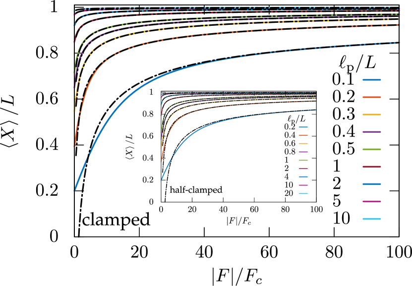
Figure 4: End-to-end distance in the direction of the force for pulling of clamped and half-clamped (inset) polymers with different persistence lengths. We use the critical buckling force $F_{c}$ to normalize the forces. The black-dashed lines indicate the weakly-bending approximation.

Pulled polymer: We have also evaluated numerically for the first time the force-extension relation of a pulled polymer. The case of free ends under pulling is up to a sign identical to compression, as discussed above (see Fig. 2(c)). In Fig. 4 we evaluate the analytic solution provided by Ref. Prasad et al. (2005) and compare it to the weakly-bending approximations Smith et al. (1992); Marko and Siggia (1995) for a clamped polymer,

$$\frac{\langle X\rangle}{L} =1+\frac{k_{\text{B}}T}{4L|F|}-\frac{\coth\left(L\sqrt{2|F|/\ell_{\text{p}}k_{\text{B}}T}\right)}{2\sqrt{2|F|\ell_{\text{p}}/k_{\text{B}}T}},$$ (45)

and a half-clamped polymer,

$$\frac{\langle X\rangle}{L} =1-\frac{\tanh\left(L\sqrt{2|F|/\ell_{\text{p}}k_{\text{B}}T}\right)}{2\sqrt{2|F|\ell_{\text{p}}/k_{\text{B}}T}};$$ (46)

see Appendix C for a derivation. These approximations accurately reproduce the force-extension relation of pulled stiff polymers. However, the weakly-bending assumption is not fulfilled for more flexible polymers at small forces, which display deviations from the exact solution (see Fig. 4). The force-extension relation of a (half-) clamped polymer exhibits qualitatively similar behavior to that of a free polymer, and aligns along the direction of the applied force.

IV Thermodynamic properties

In addition to the elastic behavior, we discuss the thermodynamic properties in terms of the excess entropy

$$\Delta S(T,F) =-\frac{\partial}{\partial T}\left[G(T,F)-G(T,F=0)\right],$$ (47)

and the excess heat capacity $\Delta C_{F}=T(\partial\Delta S/\partial T)_{F}$ in terms of our exact solution.

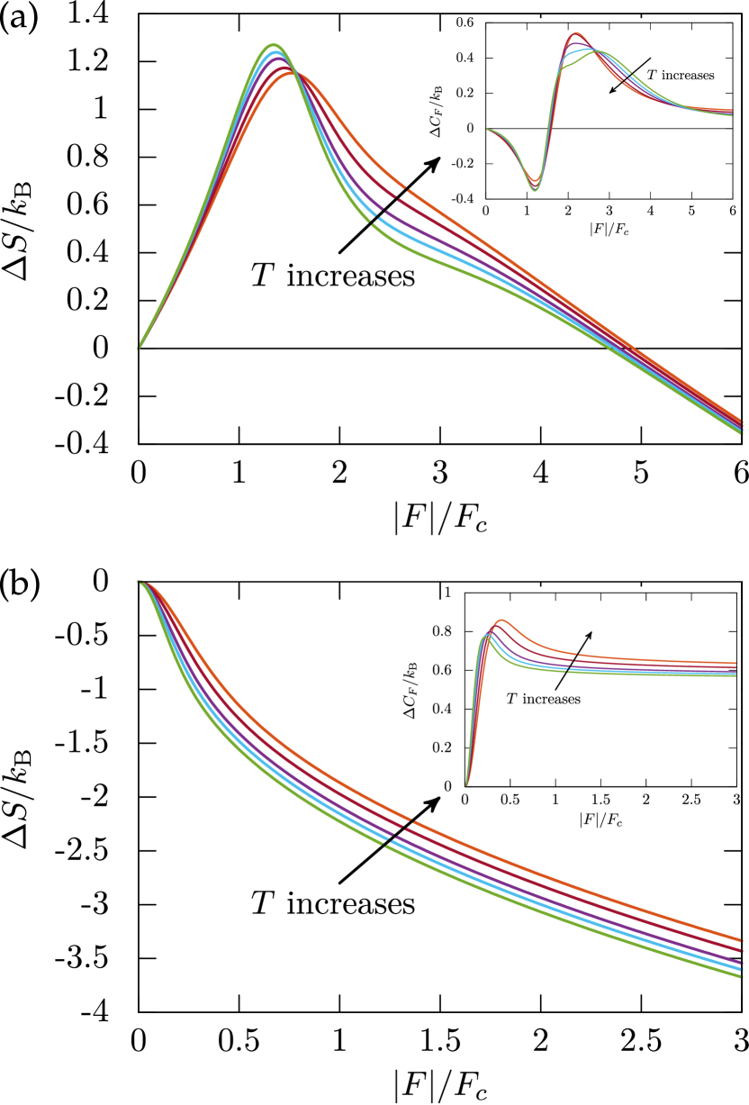
Figure 5: Excess entropy $\Delta S$ and excess heat capacity $\Delta C_{F}$ (inset) for (a) clamped and (b) free polymers as a function of the force $|F|/F_{c}$. Temperature enters via $\ell_{\text{p}}/L=2\kappa/Lk_{\text{B}}T=1.4,\ 1.7,\ 2.0,\ 2.2,\ 2.5$.

For clamped polymers, we observe an increase of the excess entropy $\Delta S$ at small forces and a decrease at forces exceeding the Euler buckling force $|F|\gtrsim F_{c}$ (see Fig. 5 (a)). Thus, by applying a small force the number of accessible configurations of the polymer is increased, which reflects that by the S-shaped configurations the fluctuations in the direction perpendicular to the force become more important. Yet, for strong forces the excess entropy decreases again and eventually even becomes negative. In fact, the simulations show that for these strong forces the clamping suppresses the undulations of the contour.

The temperature dependence of the excess entropy is encoded in the heat capacity $C_{F}(T,F)$. We find that the excess heat capacity is negative for forces $|F|\lesssim F_{c}$, whereas it becomes positive and displays a maximum for larger forces; see Fig. 5 (a) (inset). Thus, the initial increase of fluctuations upon compression is less important for more flexible polymers, while the suppression for large forces is more relevant for stiffer polymers.

Qualitatively similar results are obtained for half-clamped polymers both for the excess entropy and the excess heat capacity (not shown).

In contrast, free polymers behave qualitatively differently in terms of their thermodynamic properties. In particular, the excess entropy $\Delta S$ always decreases monotonically with increasing force (see Fig. 5 (b)). Here the polymer reverses direction and is effectively under tension, such that the force suppresses the thermal undulations and the polymer straightens out. The corresponding excess heat capacity $\Delta C_{F}$ increases and displays a prominent maximum before approaching a constant value for very large forces. As corroborated by the simulations this reflects that for more flexible polymers the thermal fluctuations are less suppressed than for stiffer ones (see Fig. 5 (b) (inset)).

V Summary and Conclusion

We have derived an analytic expression for the partition sum of a semiflexible polymer under compression within the framework of the WLC model for arbitrary stiffnesses. The partition sum is represented as an expansion in terms of Mathieu functions, which are the eigenfunctions of the associated Fokker-Planck equation. Since the eigenvalues form an ascending series to infinity, the infinite sum of decaying exponentials can be evaluated numerically (see Appendix A). Elastic properties such as the force-extension relation, the susceptibility, and thermodynamic properties in terms of the excess entropy and excess heat capacity of the polymers with different persistence lengths, have been obtained as derivatives of the exact Gibbs free energy. These properties have been discussed for different boundary conditions reflecting various experimental setups.

Our results for the force-extension relation of (half-) clamped polymers predict a smooth crossover from an equilibrated, almost straight rod to a buckled configuration. Interestingly, the force-extension curves intersect in the vicinity of the classical Euler buckling instability. Therefore, stiffer polymers resist more strongly for small forces, yet at forces larger than the buckling force they yield more strongly than flexible ones. Furthermore, the susceptibilities display a maximum in the vicinity of the classical Euler buckling force and by the fluctuation-response theorem this implies that the fluctuations of the projected mean end-to-end distance become most important here. Our analysis reveals that for large forces the weakly-bending approximation breaks down, as is apparent already for a classical elastic rod. Therefore the weakly-bending approximation remains valid only for large persistence lengths $\ell_{\text{p}}\gg L$ but is also restricted to small compression forces $|F|\lesssim F_{c}$.

In contrast, a free polymer cannot resist a compression force, rather it rotates and aligns with the applied force. Therefore, our solution for this case reproduces the well-studied setup of a semiflexible polymer under tension.

Apart from the weakly-bending approximation Baczynski et al. (2007), also different approximation schemes have been elaborated earlier to understand the behavior of rather stiff polymers close to the buckling transition. These studies have incorporated corrections by thermal fluctuation to the theory of the classical Euler buckling instability Lee et al. (2007); Emanuel et al. (2007), which capture quantitatively the force-extension relation for forces much smaller and much larger than the critical Euler buckling force $F_{c}$ and compare it to simulations of semiflexible polymers modeled by a bead-spring chain Emanuel et al. (2007). Including the lowest-order quartic mode in the fluctuations predict qualitatively the same behavior as our analytical theory for planar inextensible polymers close to the critical Euler buckling instability Lee et al. (2007). In addition, the buckling behavior of extensible polymers is also predicted to delay the buckling transition within the regime of small thermal fluctuations Bedi and Mao (2015). Alternatively to existing literature, one can also start from the probability distribution of a semiflexible polymer, which has been elaborated in the weakly-bending regime Wilhelm and Frey (1996) and within a mean-field approach for filament inextensibility Blundell and Terentjev (2009a), to compute approximately the force-extension relation.

However, these approximations Wilhelm and Frey (1996); Baczynski et al. (2007); Lee et al. (2007); Emanuel et al. (2007); Bedi and Mao (2015) remain valid for stiff polymers or away from the buckling transition only, as thermal fluctuations increase drastically for more flexible polymers at the maximum of the susceptibility. In contrast, our analytical theory provides the force-extension relation for the full range of semiflexible polymers.

Also for pulled semiflexible polymers a lot of work has been done in elaborating the force-extension relation Meng and Terentjev (2017), ranging from weakly-bending approximations Smith et al. (1992); Marko and Siggia (1995) to various approaches to account for the inextensibility of a wormlike chain MacKintosh et al. (1995); Ha and Thirumalai (1997); Palmer and Boyce (2008); Blundell and Terentjev (2009b). Here, we have evaluated for the first time the force-extension relation of pulled polymers using the analytical solution provided by Ref. Prasad et al. (2005), where up to now only approximations of the fore-extension relations of rather flexible polymers have been discussed. As we have shown in Appendix A, for flexible polymers the numerical evaluation of the partition sum reduces to a few terms, and can therefore be approximated due to the properties of the eigenvalues by the first term only, as has been observed earlier Prasad et al. (2005). However, for increasing stiffness of the polymer more terms contribute to the partition sum, the approximation fails and the full solution is required to accurately reproduce these elastic properties. In the limiting case of stiff polymers, we find excellent agreement with the weakly-bending approximation for all forces (see Fig. 4).

We anticipate, that our results serve as a reference for experimentally measured force-extension relations, and allow determining the persistence length for a broad range of semiflexible polymers. We have provided tables (see Supplemental Material [SeeSupplementalMaterialat\url{http://link.aps.org/supplemental/10.1103/PhysRevE.95.052501}fortablesoftheforce-extensionrelations]supplement) containing the numerical evaluation of the force-extension relation for semiflexible polymers subject to compression as well as pulling forces, in order to make the developed theory accessible and applicable to experimental observations.

Mathematically, the partition sum can be viewed as the Laplace transform of the distribution of the projected end-to-end distance. Therefore, the distribution can be obtained in principle by an inverse Laplace transform; however, this is numerically an ill-posed problem. Consequently, one should rather consider the characteristic function, i.e., the Fourier transform of the distribution, which is obtained formally by analytic continuation in the force to complex values. The Mathieu functions and the eigenvalues in this case can still be obtained numerically by solving a matrix eigenvalue problem. This approach has been applied recently for the mathematical analog of a self-propelled particle Kurzthaler et al. (2016).

Our solution method is not restricted to the plane but can be extended to three dimensions. There the Mathieu functions of the eigenvalue problem are replaced by generalized spheroidal wave functions Leitmann et al. (2016); Kurzthaler et al. (2016). Similarly, our approach can be extended in principle to account for a spontaneous curvature such that the classical reference system consists of a circular arc.

The equilibrium single-polymer behavior under tension or compression plays a crucial role as input for elastic properties of networks, and the regime of strong compression close to buckling may be useful to characterize the mechanical stability of such networks MacKintosh et al. (1995); Kroy and Frey (1996); Storm et al. (2005); Claessens et al. (2006); Chaudhuri et al. (2007); Huisman et al. (2008); Carrillo et al. (2013); Razbin et al. (2015); Amuasi et al. (2015); Plagge et al. (2016). In particular, networks are often modeled as entangled solutions of single semiflexible polymers with entanglement points, where they cross or loop each other, branching points or cross-links MacKintosh et al. (1995); Kroy and Frey (1996); Storm et al. (2005); Huisman et al. (2008); Carrillo et al. (2013); Razbin et al. (2015); Amuasi et al. (2015); Plagge et al. (2016). Already in equilibrium, single polymers experience a stretching or compression force induced by the surrounding network, and consequently the mean distance between, for example, two cross-links differs from the contour length of the polymers. Here, our theoretical predictions for the elastic properties of semiflexible polymers subject to different boundary conditions, which depend on the properties of the entanglement points or cross-links, allow adequate modeling and predict the equilibrium properties of polymer networks. Furthermore, exposing the network to mechanical stresses strongly depends on the force-extension relation of these individual filaments and crucially determines their elastic response. Up to now only approximate force-extension relations have been applied in the analysis of networks MacKintosh et al. (1995); Kroy and Frey (1996); Storm et al. (2005); Huisman et al. (2008); Carrillo et al. (2013); Amuasi et al. (2015), whereas our characterization of (half-)clamped and free semiflexible polymers allows analyzing the elasticity of inhomogeneous networks composed of filaments with arbitrary stiffnesses. In particular, the clamped boundary conditions might serve as a starting point for modeling polymers connected by crosslinks, where their orientation is fixed due to the specific bonds. Differently, weaker entanglements can be accounted for by applying half-clamped boundary conditions, where one end of the polymer is allowed to rotate freely. Hence, the theoretical predictions can be incorporated by using the tables provided in the Supplemental Material sup in further modeling studies of networks, which would not alter the computational cost of simulations significantly.

Similarly, the equilibrium behavior in free space constitutes the reference for the relevant case of semiflexible polymers immersed in a dense crowded medium Schöbl et al. (2014); Keshavarz et al. (2016); Leitmann et al. (2016). Furthermore, the equilibrium properties should serve as the basis also for dynamic studies Hallatschek et al. (2007a, b); Obermayer et al. (2009), in particular, the pseudodynamics we have derived here constitutes a convenient starting point to investigate the relaxation of undulation modes in the regime where the weakly-bending approximation is no longer valid.

Appendix A Numerical evaluation

Here, we discuss the numerical evaluation of the partition sums in Eqs. (26), (27), and (28), which are sums of relaxing exponentials with respect to the length $L$. Yet, the coefficients, i.e. the Mathieu functions ($\text{ce}_{2n}(q,x)$ and $\text{se}_{2n+2}(q,x)$), as well as the exponents, i.e. the eigenvalues of the Mathieu functions ($a_{2n}(q)$ and $b_{2n+2}(q)$), are non-monotonic functions with respect to the force $F$; see Fig. 6.

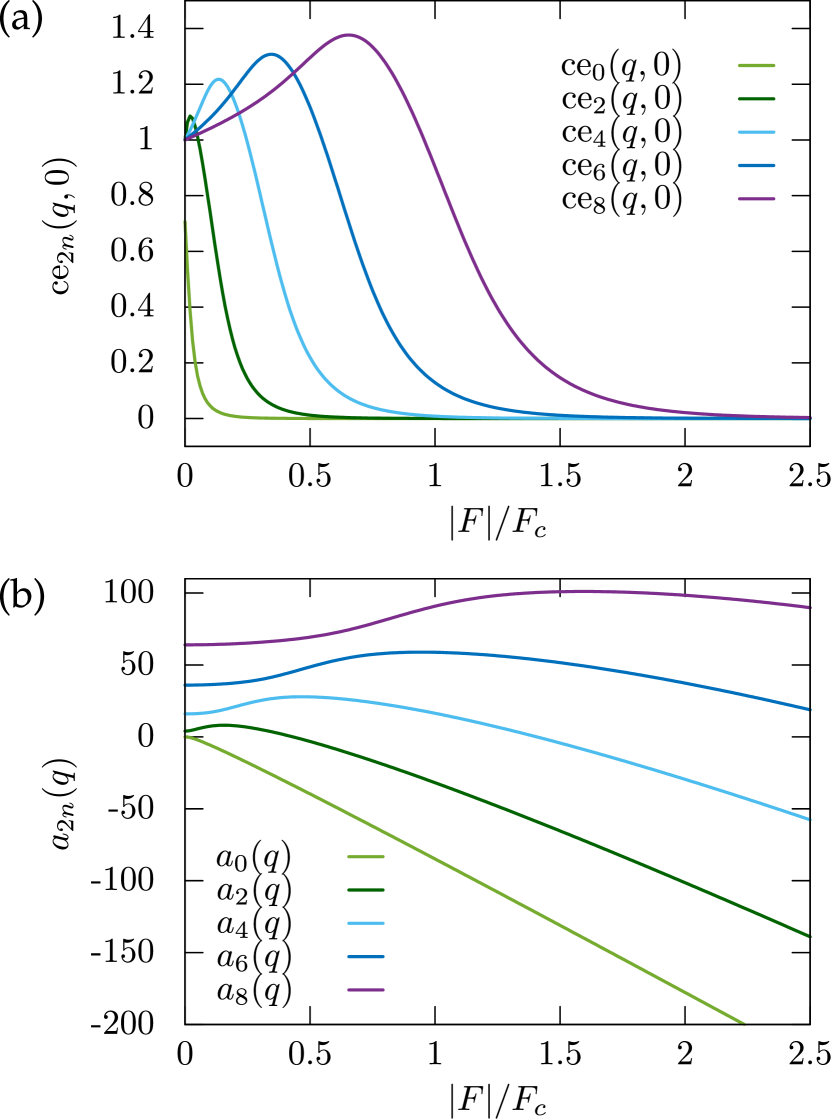
Figure 6: (a) Even Mathieu functions $\text{ce}_{2n}(q,0)$ and (b) corresponding eigenvalues $a_{2n}(q)$ with deformation parameter $q=2|f|\ell_{\text{p}}$, reduced force $f=F/k_{\text{B}}T$, and persistence length $\ell_{\text{p}}=10L$. Here, $F_{c}=\pi^{2}\kappa/L^{2}$ denotes the critical Euler buckling force of a clamped polymer.

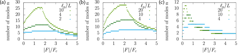
Figure 7: Number of modes $n$ required to achieve an accuracy of $|\langle X\rangle_{n+1}-\langle X\rangle_{n}|/L<10^{-8}$ with respect to the force $F$ for a clamped (a), half-clamped (b), and free polymer (c) of different persistence lengths $\ell_{\text{p}}$. Here, $F_{c}=\pi^{2}\kappa/(\gamma L)^{2}$ denotes the critical Euler buckling force. In (c) we use $\gamma=2$ in $F_{c}$ to normalize the forces.

In particular, we find, that the zeroth eigenvalue, $a_{0}(q)$, remains negative for all forces, whereas the second, $a_{2}(q)$, and fourth eigenvalues, $a_{4}(q)$, change sign within the parameter range considered. The other eigenvalues remain positive and increase with increasing mode $n$ for all relevant forces (see Fig. 6 (b)). Consequently, the higher modes of the partition sum become exponentially suppressed, and therefore induce a natural cut-off of the infinite series [Eqs. (26), (27), and (28)].

Moreover, with increasing mode $n$ the Mathieu functions become more important at intermediate and larger forces (see Fig. 6 (a)), and therefore many modes are expected to contribute to the partition sum. Interestingly, we observe that the number of modes necessary to achieve a desired accuracy of the elastic properties highly depends on the force.

As an example, we consider the mean end-to-end distance $\langle X\rangle$, and determine the number of modes necessary to obtain the accuracy $|\langle X\rangle_{n+1}-\langle X\rangle_{n}|/L<10^{-8}$, where $\langle X\rangle_{n}$ denotes the mean end-to-end distance with $n$ included modes. For a clamped and a half-clamped polymer, the number of modes increases and assumes a maximum in the vicinity of the critical Euler buckling force, and decreases again for larger forces; see Figs. 7(a) and (b). Similarly, for a free polymer the number of modes also increases, yet at smaller forces, and decreases for large forces [Fig. 7(c)].

In addition, the number of modes rises drastically for stiffer polymers, which makes numerical evaluation more tedious. Furthermore, the number of modes for half-clamped boundary conditions is largest, whereas about half the modes are required for a free polymer.

Appendix B Derivation of the pseudo dynamics

In general, equations of motion in terms of stochastic differential equations can be derived from the Fokker-Planck equation of the stochastic process Gardiner (2009). At this stage, only the equilibrium distribution of the polymer subject to an external compression force is known and an equation of motion for the probability density needs to be formulated. Therefore, we construct a Fokker-Planck equation starting with the requirement that the known equilibrium distribution of the WLC model coincides with the stationary distribution of the stochastic process. Therefore, we discretize the polymer equidistantly in terms of the positions of the beads $\{\mathbf{R}_{i}\}_{i=0}^{N}$ and corresponding tangent vectors $\{\mathbf{u}_{i}\}_{i=0}^{N-1}$, where $\mathbf{u}_{i}=(\mathbf{R}_{i+1}-\mathbf{R}_{i})N/L$ with unit length $|\mathbf{u}_{i}|=1$. The discretized Hamiltonian takes the form

$$\frac{\mathcal{H}(\{\mathbf{u}_{i}\}_{i=0}^{N-1})}{k_{\text{B}}T} =\frac{\hat{\ell}_{\text{p}}}{4}\sum_{i=0}^{N-2}(\mathbf{u}_{i+1}-\mathbf{u}_{i})^{2}-\hat{f}\sum_{i=0}^{N-1}\mathbf{e}\cdot\mathbf{u}_{i},\$$ (48)

where $\hat{\ell}_{\text{p}}=\ell_{\text{p}}N/L$ and $\hat{f}=fL/N$ denote the scaled persistence length and force ($\hat{f}>0$ for tension and $\hat{f}<0$ for compression), respectively.

To fulfill the inextensibility constraint, we parametrize the orientation $\mathbf{u}_{i}=(\cos\varphi_{i},\sin\varphi_{i})^{T}$ in terms of the polar coordinates $\{\varphi_{i}\}\equiv\{\varphi_{i}\}_{i=0}^{N-1}$ measured relative to the fixed direction $\mathbf{e}$ of the force. Therefore, the probability density in equilibrium is given by

$$\mathbb{P}_{\text{eq}}(\{\varphi_{i}\}) =Z^{-1}\exp\left(-\frac{\mathcal{H}(\{\varphi_{i}\})}{k_{\text{B}}T}\right),$$ (49)

such that $\int\left[\prod_{i=0}^{N-1}\mathrm{d}\varphi_{i}\right]\mathbb{P}_{\text{eq}}(\{\varphi_{i}\})=1$.

The discretized Hamiltonian in polar coordinates reads

$$\frac{\mathcal{H}(\{\varphi_{i}\})}{k_{\text{B}}T} =\frac{\hat{\ell}_{p}}{2}\sum_{i=0}^{N-2}[1-\cos(\varphi_{i+1}-\varphi_{i})]-\hat{f}\sum_{i=0}^{N-1}\cos\varphi_{i},$$ (50)

Next we derive the Fokker-Planck equation describing the time evolution of the conditional probability density $\mathbb{P}\equiv\mathbb{P}(\{\varphi_{i}\},t|\{\varphi_{i}^{0}\})$ to find a discretized polymer with orientations $\{\varphi_{i}\}$ at time $t$, given that it was oriented with $\{\varphi_{i}^{0}\}$ at time $t=0$. It is expressed by

$$\partial_{t}\mathbb{P}=-\sum_{i=0}^{N-1}\partial_{\varphi_{i}}[U^{i}(\{\varphi_{i}\})\mathbb{P}],$$ (51)

where the velocity of the probability current is obtained by the friction law, $U^{i}(\{\varphi_{i}\})=\sum_{k}K^{ik}(\{\varphi_{i}\})F_{k}(\{\varphi_{i}\})$. We choose for simplicity $\mathbf{K}=N\xi_{r}^{-1}\mathbb{I}$, which denotes the rotational mobility tensor and $\mathbf{F}$ the forces,

$$F_{k} =-\partial_{\varphi_{k}}\mathcal{H}-k_{\text{B}}T\partial_{\varphi_{k}}\ln\mathbb{P}.$$ (52)

Here, the first term corresponds to the mechanical forces while the second accounts for the thermal Brownian forces. Thus one verifies that the equilibrium distribution $\mathbb{P}_{\text{eq}}$ corresponds to the stationary distribution, $\partial_{t}\mathbb{P}_{\text{eq}}=0$. Collecting results we find for the time evolution of the conditional probability density,

$$\partial_{t}\mathbb{P} =\hat{D}_{\text{rot}}\sum_{i=0}^{N-1}\Bigl{\{}\partial_{\varphi_{i}}\Bigl{[}\frac{\hat{\ell}_{\text{p}}}{2}\left(\sin(\varphi_{i}-\varphi_{i-1})-\sin(\varphi_{i+1}-\varphi_{i})\right)$$

$$+\hat{f}\sin\varphi_{i}\Bigr{]}\mathbb{P}+\partial^{2}_{\varphi_{i}}\mathbb{P}\Bigr{\}},$$ (53)

with scaled rotational diffusion coefficient $\hat{D}_{\text{rot}}=Nk_{\text{B}}T/\xi_{\text{r}}$ and initial condition

$$\mathbb{P}(\{\varphi_{i}\},t=0|\{\varphi_{i}^{0}\},0) =\prod_{i=0}^{N-1}\delta(\varphi_{i}-\varphi_{i}^{0}\text{ mod }2\pi).$$ (54)

Starting from the Fokker-Planck equation [Eq. 53] standard methods Gardiner (2009) are used to obtain the Langevin equations for the angles, governing the pseudodynamics of a semiflexible, discretized polymer,

$$\mathrm{d} \varphi_{i}(t)=-\hat{D}_{\text{rot}}\Bigl{[}\frac{\hat{\ell}_{\text{p}}}{2}\left(\sin(\varphi_{i}-\varphi_{i-1})-\sin(\varphi_{i+1}-\varphi_{i})\right)$$

$$+\hat{f}\sin\varphi_{i}\Bigr{]}\mathrm{d}t+\sqrt{2\hat{D}_{\text{rot}}}\mathrm{d}\omega_{i}(t),$$ (55)

where $\mathrm{d}\omega_{i}(t)$ is the increment of a Gaussian white noise process $\omega_{i}(t)$ with zero mean $\langle\omega_{i}(t)\rangle=0$ and delta-correlated variance $\langle\omega_{i}(t)\omega_{j}(s)\rangle=\delta_{ij}\delta(t-s)$ for $i,j=0,\ldots,N-1$. These equations can be transformed by It$\bar{\text{o}}$’s lemma Gardiner (2009) to the equations for the tangent vectors in Eq. (40).

Appendix C Force-extension relation for a pulled polymer in the weakly-bending regime

In the weakly-bending regime of a pulled polymer, $f=|f|$, we can approximate Eq. (17) by

$$\partial_{s}Z(\varphi,s|\varphi_{0},0) =\left[\frac{1}{\ell_{\text{p}}}\partial^{2}_{\varphi}+|f|(1-\frac{1}{2}\varphi^{2})\right]Z(\varphi,s|\varphi_{0},0),$$ (56)

and use the Gaussian ansatz

$$Z(\varphi,s|\varphi_{0},0)=\exp\left[-M(s)\varphi^{2}/2+\Gamma(s)\right].$$ (57)

Then the inverse variance $M(s)$ and the normalization $\Gamma(s)$ have to fulfill the equations of motion

$$\frac{\mathrm{d}}{\mathrm{d}s}M(s) =|f|-2\frac{M(s)^{2}}{\ell_{\text{p}}},$$ (58)

$$\frac{\mathrm{d}}{\mathrm{d}s}\Gamma(s) =|f|-\frac{M(s)}{\ell_{\text{p}}}.$$ (59)

Using the initial condition $Z(\varphi,s=0|\varphi_{0}=0,0)=\delta(\varphi)$, the solutions of these differential equations read

$$M(s) =\sqrt{\frac{|f|\ell_{\text{p}}}{2}}\coth\left(\sqrt{\frac{2|f|}{\ell_{\text{p}}}}s\right),$$ (60)

$$\Gamma(s) =|f|s-\frac{1}{2}\ln\sinh\left(\sqrt{\frac{2|f|}{\ell_{\text{p}}}}s\right)+\frac{1}{4}\ln\left(\frac{\ell_{\text{p}}|f|}{8\pi^{2}}\right).$$ (61)

To obtain the partition sum for a half-clamped polymer with contour length $L$, we average over the final orientation,

$$Z(L|\varphi_{0},0) \approx\int_{-\infty}^{\infty}\mathrm{d}\varphi_{L}\exp\left[-M(L)\varphi_{L}^{2}/2+\Gamma(L)\right]$$

$$=\exp\left[\Gamma(L)\right]\sqrt{\frac{2\pi}{M(L)}},$$ (62)

which is correct if the angular fluctuations are small, $M(s)\gg 1$. This is fulfilled for stiff polymers $L/\ell_{\text{p}}\ll 1$ or strong pulling $\ell_{\text{p}}|f|\gg 1$. Finally, we obtain the force-extension relations for (half-) clamped polymers in the weakly-bending regime by taking the derivative of the Gibbs free energy [Eq. (7)] with respect to the force (see Sec. II).

References

- Sackmann (1994) E. Sackmann, Macromolecular Chemistry and Physics 195, 7 (1994).
- Brangwynne et al. (2006) C. P. Brangwynne, F. C. MacKintosh, S. Kumar, N. A. Geisse, J. Talbot, L. Mahadevan, K. K. Parker, D. E. Ingber, and D. A. Weitz, The Journal of cell biology 173, 733—741 (2006).
- Bausch and Kroy (2006) A. Bausch and K. Kroy, Nature Physics 2, 231 (2006).
- Fletcher and Mullins (2010) D. A. Fletcher and R. D. Mullins, Nature 463, 485 (2010).
- Lieleg et al. (2010) O. Lieleg, M. M. A. E. Claessens, and A. R. Bausch, Soft Matter 6, 218 (2010).
- Nolting et al. (2014) J.-F. Nolting, W. Möbius, and S. Köster, Biophysical Journal 107, 2693 (2014).
- MacKintosh et al. (1995) F. C. MacKintosh, J. Käs, and P. A. Janmey, Phys. Rev. Lett. 75, 4425 (1995).
- Kroy and Frey (1996) K. Kroy and E. Frey, Phys. Rev. Lett. 77, 306 (1996).
- Storm et al. (2005) C. Storm, J. J. Pastore, F. C. MacKintosh, T. C. Lubensky, and P. A. Janmey, Nature 435, 191 (2005).
- Claessens et al. (2006) M. Claessens, R. Tharmann, K. Kroy, and A. Bausch, Nature Physics 2, 186 (2006).
- Chaudhuri et al. (2007) O. Chaudhuri, S. H. Parekh, and D. A. Fletcher, Nature 445, 295 (2007).
- Huisman et al. (2008) E. M. Huisman, C. Storm, and G. T. Barkema, Phys. Rev. E 78, 051801 (2008).
- Carrillo et al. (2013) J.-M. Y. Carrillo, F. C. MacKintosh, and A. V. Dobrynin, Macromolecules 46, 3679 (2013).
- Razbin et al. (2015) M. Razbin, M. Falcke, P. Benetatos, and A. Zippelius, Physical Biology 12, 046007 (2015).
- Amuasi et al. (2015) H. Amuasi, C. Heussinger, R. Vink, and A. Zippelius, New Journal of Physics 17, 083035 (2015).
- Plagge et al. (2016) J. Plagge, A. Fischer, and C. Heussinger, Phys. Rev. E 93, 062502 (2016).
- Ratner et al. (2004) B. Ratner, A. Hoffman, F. Schoen, and J. Lemons, Biomaterials Science: An Introduction to Materials in Medicine (Elsevier Academic Press, San Diego, London, 2004).
- Ratner and Bryant (2004) B. D. Ratner and S. J. Bryant, Annual Review of Biomedical Engineering 6, 41 (2004).
- Hugel and Seitz (2001) T. Hugel and M. Seitz, Macromolecular Rapid Communications 22, 989 (2001).
- Ott et al. (1993) A. Ott, M. Magnasco, A. Simon, and A. Libchaber, Phys. Rev. E 48, R1642 (1993).
- Broedersz and MacKintosh (2014) C. P. Broedersz and F. C. MacKintosh, Rev. Mod. Phys. 86, 995 (2014).
- Razbin et al. (2016) M. Razbin, P. Benetatos, and A. Zippelius, Phys. Rev. E 93, 052408 (2016).
- Ashkin (1997) A. Ashkin, Proceedings of the National Academy of Sciences 94, 4853 (1997).
- Mehta et al. (1999) A. D. Mehta, M. Rief, J. A. Spudich, D. A. Smith, and R. M. Simmons, Science 283, 1689 (1999).
- Gosse and Croquette (2002) C. Gosse and V. Croquette, Biophysical Journal 82, 3314 (2002).
- Kuzumaki and Mitsuda (2006) T. Kuzumaki and Y. Mitsuda, Japanese Journal of Applied Physics 45, 364 (2006).
- Janshoff et al. (2000) A. Janshoff, M. Neitzert, Y. Oberdörfer, and H. Fuchs, Angewandte Chemie International Edition 39, 3212 (2000).
- Saleh (2015) O. A. Saleh, The Journal of chemical physics 142, 194902 (2015).
- Marko and Siggia (1995) J. F. Marko and E. D. Siggia, Macromolecules 28, 8759 (1995).
- Bouchiat et al. (1999) C. Bouchiat, M. Wang, J.-F. Allemand, T. Strick, S. Block, and V. Croquette, Biophysical Journal 76, 409 (1999).
- Bustamante et al. (2000) C. Bustamante, S. B. Smith, J. Liphardt, and D. Smith, Current Opinion in Structural Biology 10, 279 (2000).
- Liu and Pollack (2002) X. Liu and G. H. Pollack, Biophysics Journal 83, 2705 (2002).
- Kellermayer et al. (1997) M. S. Z. Kellermayer, S. B. Smith, H. L. Granzier, and C. Bustamante, Science 276, 1112 (1997).
- Sun et al. (2002) Y.-L. Sun, Z.-P. Luo, A. Fertala, and K.-N. An, Biochemical and Biophysical Research Communications 295, 382 (2002).
- Kratky and Porod (1949) O. Kratky and G. Porod, Recueil des Travaux Chimiques des Pays-Bas 68, 1106 (1949).
- Wilhelm and Frey (1996) J. Wilhelm and E. Frey, Phys. Rev. Lett. 77, 2581 (1996).
- Hamprecht et al. (2004) B. Hamprecht, W. Janke, and H. Kleinert, Physics Letters A 330, 254 (2004).
- Spakowitz et al. (2004) A. J. Spakowitz, , and Z.-G. Wang, Macromolecules 37, 5814 (2004).
- Spakowitz and Wang (2005) A. J. Spakowitz and Z.-G. Wang, Phys. Rev. E 72, 041802 (2005).
- Mehraeen et al. (2008) S. Mehraeen, B. Sudhanshu, E. F. Koslover, and A. J. Spakowitz, Phys. Rev. E 77, 061803 (2008).
- Taute et al. (2008) K. M. Taute, F. Pampaloni, E. Frey, and E.-L. Florin, Phys. Rev. Lett. 100, 028102 (2008).
- Pampaloni et al. (2006) F. Pampaloni, G. Lattanzi, A. Jonáš, T. Surrey, E. Frey, and E.-L. Florin, Proceedings of the National Academy of Sciences 103, 10248 (2006).
- Prasad et al. (2005) A. Prasad, Y. Hori, and J. Kondev, Phys. Rev. E 72, 041918 (2005).
- Baczynski et al. (2007) K. Baczynski, R. Lipowsky, and J. Kierfeld, Phys. Rev. E 76, 061914 (2007).
- Emanuel et al. (2007) M. Emanuel, H. Mohrbach, M. Sayar, H. Schiessel, and I. M. Kulić, Phys. Rev. E 76, 061907 (2007).
- Lee et al. (2007) N. K. Lee, A. Johner, and S. C. Hong, The European Physical Journal E 24, 229 (2007).
- Bedi and Mao (2015) D. S. Bedi and X. Mao, Phys. Rev. E 92, 062141 (2015).
- Ghosh et al. (2007) A. Ghosh, J. Samuel, and S. Sinha, Phys. Rev. E 76, 061801 (2007).
- Doi and Edwards (1986) M. Doi and S. F. Edwards, The Theory of Polymer Dynamics (Oxford Science Publications, 1986).
- Landau and Lifshitz (1986) L. D. Landau and E. Lifshitz, Course of Theoretical Physics 7 (1986).
- Kleinert (2009) H. Kleinert, Path Integrals in Quantum Mechanics, Statistics, Polymer Physics, and Financial Markets, EBL-Schweitzer (World Scientific, Singapore, 2009).
- Aldrovandi and Ferreira (1980) R. Aldrovandi and P. L. Ferreira, American Journal of Physics 48, 660 (1980).
- (53) DLMF, “NIST Digital Library of Mathematical Functions,” http://dlmf.nist.gov/, Release 1.0.13 of 2016-09-16, online companion to Olver et al. (2010).
- Olver et al. (2010) F. W. J. Olver, D. W. Lozier, R. F. Boisvert, and C. W. Clark, eds., NIST Handbook of Mathematical Functions (Cambridge University Press, New York, NY, 2010) print companion to DLMF .
- Wolfram Research (2016) I. Wolfram Research, “Mathematica 10.4,” (2016).
- Smith et al. (1992) S. B. Smith, L. Finzi, and C. Bustamante, Science 258, 1122 (1992).
- Blundell and Terentjev (2009a) J. R. Blundell and E. M. Terentjev, Soft Matter 5, 4015 (2009a).
- Meng and Terentjev (2017) F. Meng and E. M. Terentjev, Polymers 9, 52 (2017).
- Ha and Thirumalai (1997) B.-Y. Ha and D. Thirumalai, The Journal of chemical physics 106, 4243 (1997).
- Palmer and Boyce (2008) J. S. Palmer and M. C. Boyce, Acta Biomaterialia 4, 597 (2008).
- Blundell and Terentjev (2009b) J. Blundell and E. Terentjev, Macromolecules 42, 5388 (2009b).
- (62) .
- Kurzthaler et al. (2016) C. Kurzthaler, S. Leitmann, and T. Franosch, Scientific Reports 6, 36702 (2016).
- Leitmann et al. (2016) S. Leitmann, F. Höfling, and T. Franosch, Phys. Rev. Lett. 117, 097801 (2016).
- Schöbl et al. (2014) S. Schöbl, S. Sturm, W. Janke, and K. Kroy, Phys. Rev. Lett. 113, 238302 (2014).
- Keshavarz et al. (2016) M. Keshavarz, H. Engelkamp, J. Xu, E. Braeken, M. B. J. Otten, H. Uji-i, E. Schwartz, M. Koepf, A. Vananroye, J. Vermant, R. J. M. Nolte, F. De Schryver, J. C. Maan, J. Hofkens, P. C. M. Christianen, and A. E. Rowan, ACS Nano 10, 1434 (2016).
- Hallatschek et al. (2007a) O. Hallatschek, E. Frey, and K. Kroy, Phys. Rev. E 75, 031905 (2007a).
- Hallatschek et al. (2007b) O. Hallatschek, E. Frey, and K. Kroy, Phys. Rev. E 75, 031906 (2007b).
- Obermayer et al. (2009) B. Obermayer, W. Möbius, O. Hallatschek, E. Frey, and K. Kroy, Physical Review E 79, 021804 (2009).
- Gardiner (2009) C. Gardiner, Stochastic Methods: A Handbook for the Natural and Social Sciences, Springer Series in Synergetics (Springer Berlin Heidelberg, 2009).