The origin of fine structure in magnetization curve of $\alpha$-CoV₂O₆

Abstract

Multiple field-induced plateaus in $\alpha$-CoV₂O₆ at low temperatures were revealed earlier by M. Lenertz et al. [J. Phys. Chem. C 115, 17190 (2011)] and carefully investigated recently by M. Nandi and P. Mandal [J. Appl. Phys. 119, 133904 (2016)]. Four equidistant steps were observed in the magnetization curve. We present a model to describe this phenomenon. A magnetic structure of this substance is formed by highly anisotropic triangular lattice of Ising chains running along the $\bf{b}$ axis. Due to a three-fold degeneracy of three-sublattice magnetic ordering, domain boundaries appear. Their transformation under magnetic field variation leads to two additional steps in the 1/3 magnetization plateau and gives rise to complex magnetic behavior observed experimentally. The domain structure in $\alpha$-CoV₂O₆ occurs to be strongly anisotropic because a lifetime of the metastable states depends greatly on the configuration orientation. A strong dependence of the magnetization curve on magnetic field sweep time is predicted.

Ising spin-chain compounds have drawn considerable attention due to unusual magnetic behavior Kudasov et al. (2012); Mekata (1977); Maignan et al. (2004); Hardy et al. (2006). A complicated hierarchy of magnetic interactions determines main features of these systems. The strongest of them act along the chains. That is why in the framework of the rigid-chain model Kudasov (2006) the chains are considered as elements of the magnetic structure with two possible magnetization states. Weak antiferromagnetic (AFM) interchain interactions in the triangular lattice of chains lead to the geometric frustration and complex phase diagram. At high temperatures a partially disordered antiferromagnetic (PDA) phase appears Mekata (1977). Very weak next-to-the-nearest interchain interactions or anisotropy partially lift the degeneracy of the ground state and produce various low-temperature magnetic structures: the three-sublattice (3SL) one in CsCoCl₃ and related compounds, stripes in Sr₅Rh₄O₁₂ Cao et al. (2007); Kudasov (2008), and strongly disordered Wannier’s state Wannier (1950) in Ca₃Co₂O₆ Maignan et al. (2004); Hardy et al. (2004); Kudasov et al. (2008).

One of the most striking features observed in the spin-chain compounds is a multi-step magnetization curve in Ca₃Co₂O₆ Maignan et al. (2004); Hardy et al. (2004) and Sr₃HoCrO₆ Hardy et al. (2006). The plateau 1/3 at high temperatures is related to transition to the 3SL phase. At low temperatures two additional steps appear at the plateau. They are assumed to be a consequence of a three-fold degeneracy of the 3SL configuration which gives rise to a domain structure Kudasov et al. (2012, 2011). This is a long-lived metastable state which determines a slow magnetic dynamics in Ca₃Co₂O₆ Kudasov et al. (2012); Hardy et al. (2004).

In this Brief Report we discuss the multi-step behavior in CoV₂O₆ revealed in Ref. Lenertz et al. (2011) and thoroughly investigated recently Nandi and Mandal (2016). This compound crystallizes in the two allotropic forms Lenertz et al. (2011): the branneritelike monoclinic structure with the space group C2/m which is schematically shown in Fig. 1 ($\alpha$-phase) and the triclinic structure with the P-1 space group ($\gamma$-phase). They have rather similar magnetic behavior, however in the present article we discuss the $\alpha$-CoV₂O₆ only. Magnetic Co²⁺ ions in the $\alpha$ phase are placed in the well separated chains made up of edge-sharing distorted CoO₆ octahedra. The chains run along the $\bf{b}$ axis. Pentavalent vanadium ions are nonmagnetic and located in edge-shared VO₅ square-pyramids between the chains being involved in interchain magnetic interactions.

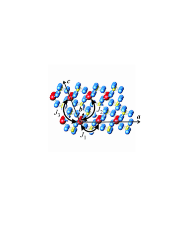
Figure 1: (color online) The crystal structure of $\alpha$-CoV₂O₆. The large red, smaller blue, and the smallest yellow spheres denote the Co²⁺, O^2-, and V⁵⁺ ions correspondingly. The arrows show interchain interactions.

Magnetic measurements of $\alpha$-CoV₂O₆ revealed an Ising-type anisotropy with the easy axis along $\bf{c}$ axis He and Cheng (2014). It arises from cooperative effects of the crystal electric field of the distorted octahedra and spin-orbit coupling Kim et al. (2012). This combination also leads to unusually high orbital moment of Co²⁺ ions. The magnetic structure is formed by the strong ferromagentic (FM) in-chain coupling between the Co²⁺ ions, and weak AFM interchain interactions. They lead to the AFM state below $T_{N}=15$ K. The lattice of the chains can be considered as a distorted 2D triangular lattice with three AFM coupling constants between the nearest neighboring chains $J_{1}$, $J_{2}$, and $J_{3}$ which act along $[100]$, $[101]$, and $[001]$ directions, respectively (see Fig. 1). The values of $J_{1}$, $J_{3}$ although are different but comparable, $J_{2}$ is much weaker than $J_{1}$ and $J_{3}$. According to Ref. Lenertz et al. (2012) the estimations of the coupling constant are $J_{1}=0.356$ meV, $J_{2}=0.051$ meV, and $J_{3}=0.463$ meV. As was shown in Ref. Saul et al. (2013) interactions between the next to the nearest neighbor are rather weak and can be omitted.

Magnetization curves of $\alpha$-CoV₂O₆ below $T_{N}$ demonstrated two steps separating plateaus with zero magnetization ($M=0$) at low magnetic field, one third of the saturation magnetization ($M=1/3$), and the saturated state ($M=1$). This structure was observed from 12 K to 5 K. The neutron scattering Markkula et al. (2012); Lenertz et al. (2012) and Monte Carlo simulation showed that the first plateau corresponds to the stripe magnetic structure, and the 1/3 plateau does to three sublattices (3SL) configurations. The Monte Carlo simulation by the Metropolis algorithm in some cases gave additional features in the 1/3 plateau. However, it should be mentioned that this technique fails to relax correctly a trial state into the equilibrium state on the AFM triangular Ising model and the Wang-Landau algorithm should be applied instead Qin et al. (2009). The Wang-Landau simulation produces the flat 1/3 plateau in case of $\alpha$-CoV₂O₆ Yao (2012).

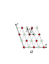
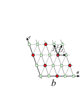
Figure 2: (color online) Magnetic structures of stripe (a) and 3SL phases. The solid (red) and dash (blue) circles denote spin-down and spin-up (along the magnetic field) chain states, repectively.

Two additional steps steps in the 1/3 plateau were revealed at very low temperatures below 5 K Lenertz et al. (2011). The four magnetization steps are equidistant on the magnetic field (1.6, 2.2, 2.8, and 3.4 T) Lenertz et al. (2011); Nandi and Mandal (2016) similarly to Ca₃Co₂O₆ despite the fact the 2D lattice of chains is strongly anisotropic. This phenomenon is worthy of thorough investigation.

The rigid-chain model for $\alpha$-CoV₂O₆ was formulated by Yao as following Yao (2012)

$$\hat{H}=\sum_{<ij>}{J_{ij}\sigma_{i}\sigma_{j}}-hM$$ (1)

where $\sigma_{i}=\pm 1$ is the $c$-axis projection of the $i$-th chain magnetic moment, $M=\sum_{i}{\sigma_{i}}$ is the total magnetization, $<\ldots>$ denotes the summation over the nearest neighboring chains only, $J_{ij}$ is a positive constant which assumes values $J_{1}$, $J_{2}$, or $J_{3}$ ($J_{1}\approx J_{3}$, $J_{2}<J_{1}$, $J_{2}<J_{3}$) depending on the bond orientation, $h$ is the magnetic field.

At the zero magnetic field the equilibrium state is the stripe structure oriented along the $[101]$ direction as shown in the Fig. 2a. While magnetic field increasing a first order transition to the 3SL phase occur at the first critical magnetic field Yao (2012)

$$h_{c1}=2(J_{1}+J_{3})-4J_{2}.$$ (2)

The 3SL structure is shown in Fig. 2b. Further increase of the magnetic field leads to the second transition to the saturated FM state at the second critical magnetic field Yao (2012)

$$h_{c2}=2(J_{1}+J_{3}+J_{2}).$$ (3)

These two critical magnetic fields form the two steps in the equilibrium magnetization curve (Fig. 3) which was observed in the temperature range between 5 and 15 K.

To discuss the multi-step behavior at low temperatures one should take into account frozen metastable states. Necessary conditions of the metastability at the zero temperature have the following form Kim et al. (2003); Kudasov (2006)

$$\sigma_{i}h_{i}\leq 0$$ (4)

where $h_{i}=\sum_{j(i)}{J_{ij}\sigma_{j}}-h$ is the effective field for the $i$-th chain. This condition should be satisfied for all the chains.

At finite temperatures the lifetime $\tau$ of a metastable state can be estimated by the Glauber theory Glauber (1963) extended to 2D and 3D lattices Buendía et al. (2004); Kudasov et al. (2012). Following to it one assumes that the chains interact not only with the nearest neighbors and external magnetic field but also with a heat reservoir. It was shown that a hard type of the Glauber dynamics describes well the slow dynamics in frustrated spin-chain system Kudasov et al. (2012, 2011); Buendía et al. (2004). In this case the probability of a spin flip of the $i$-th chain per time unit can be written down as

$$W_{i}=\frac{\alpha}{2}\left[1-\sigma_{i}\cdot\tanh\left(-\frac{h_{i}}{k_{B}T}\right)\right]$$ (5)

where $\alpha$ is the constant of the interaction of a chain with the heat reservoir, $k_{B}$ is the Boltzmann constant, $T$ is the temperature. Then the lifetime of the $i$-th chain state is $\tau_{i}=W_{i}^{-1}$. If $\tau\sim\alpha^{-1}$ the state is unstable, and $\tau>>\alpha^{-1}$ corresponds to a metastable (or stable) state.

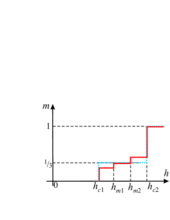
Figure 3: (color online) A schematic view of the magnetization curves of $\alpha$-CoV₂O₆ in the increasing magnetic field: the dotted (blue) and the solid (red) lines correspond to the equilibrium and metastable regimes.

There are two basic causes for the metastability just above $h_{c1}$. Firstly, using the condition Eq. (4) it is easy to show that the stripe phase still exist as a metastable state up to the magnetic field

$$h_{m1}=2(J_{1}+J_{3})-2J_{2}.$$ (6)

The 3SL structure is three-fold degenerate, and when it starts growing from few nucleation centers domain boundaries appear. Let us consider the domain boundaries lying in the (101) planes. The possible configurations are shown in Fig. 4. Since the FM bonds for the spin-down chains in domain boundaries (A and B positions) are along the $[101]$ direction with the weakest AFM coupling constant $J_{2}$ this orientation makes the most stable domain boundaries. We discuss this point below. The configurations in Fig. 4a give an excess of spin-down chains as compared with monodomain 3SL structure. That is why just above $h_{c1}$ the magnetization of the metastable state is less than that of the equilibrium one. The chains in the position B become unstable at the magnetic field determined by Eq. (6) that causes the additional step in the magnetization curve (see Fig. 3).

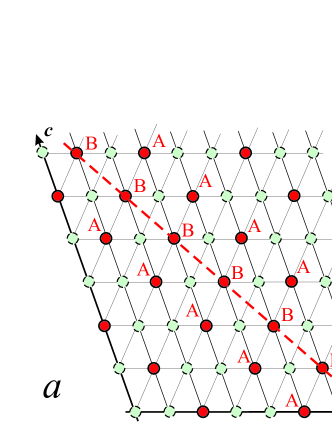
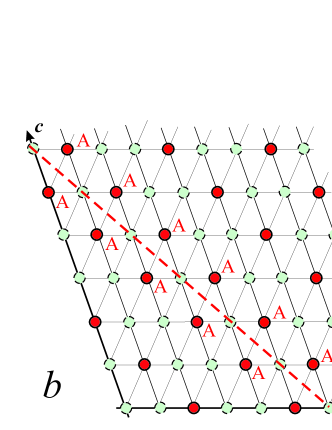
Figure 4: (color online) Two possible structures of the domain boundaries in the 3SL phase in the (101) planes. A and B denote positions of spin-down chains with two different types of the nearest-neighbor environment.

The spin-down chains in the position A in Fig. 4b remain stable up to another critical field

$$h_{m2}=2(J_{1}+J_{3}).$$ (7)

At this point half of the spin-down chains in the A-A pairs (Fig. 3) flips to the spin-up state. This gives rise to an excess of spin-up chains. Therefore, there appears a magnetization step at $h_{m2}$ and the plateau with the magnetization greater than the equilibrium one. In the range between $h_{m2}$ and $h_{c2}$ spin-down chains are stable only in case of all the six nearest neighbors are in the spin-up state.

Until now we discussed the domain boundaries lying in the $(101)$ plane. Let us consider the ones in other planes, e.g. $(100)$, and more generally other types of metastable states. Then we investigate the stability of the chain in the down state similar to the B position but with two nearest neighbors in the down positions along the $[100]$ direction (B^′ position see Fig. 5). The corresponding critical magnetic fields can be calculated by a coupling constants permutation. Then the equation Eq. (6) is replaced by $h^{\prime}_{m1}=2(J_{2}+J_{3})-2J_{1}$. If $h^{\prime}_{m1}<h_{c1}$ the B^′ states are unstable, that is they exist only if $J_{2}>2/3J_{1}$.

Let us compare the lifetime for different metastable states. The additional steps at the 1/3 plateau are observed at very low temperatures only when $k_{B}T$ is much less than any of $J_{1}$, $J_{2}$, and $J_{3}$. Then one can estimate the lifetime from Eq. (5) as $\tau_{i}\approx\alpha^{-1}\exp{(|h_{i}|/k_{B}T)}$. Therefore the lifetime is large as compared to $\alpha^{-1}$ in all the area of the metastablity except a narrow region in the vicinity of the critical field where $|h_{i}|$ is close to or less than $k_{B}T$. Applying this expression we obtain that the lifetime of a chain in the B position larger than that in the B^′ one by a factor of $\exp\left[2(J_{1}-J_{2})/(k_{B}T)\right]>>1$.

After a similar reasoning one can show that if a chain in the down state has one or two nearest neighbors in the down states then any configuration, which differs from A or B positions (e.g. A^′ or B^′ in Fig. 5), has exponentially small lifetime and therefore can be neglected.

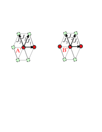
Figure 5: (color online) Examples of possible short-lived metastable configurations.

It is interesting to mention that the four-step structure in the magnetization curve can appear in the two cases only: perfect triangular lattice (Ca₃Co₂O₆) and strongly anisotropic triangular lattice ($\alpha$-CoV₂O₆). If the anisotropy is weak the critical fields for different orientation of domain boundaries slightly differ from one another. This should smear the additional steps at the plateau 1/3.

It is possible to get a new relation between the coupling constants from the model developed above:

$$\frac{h_{c2}-h_{c1}}{h_{m2}}=\frac{3J_{2}}{J_{1}+J3}.$$ (8)

From here one can see that the value of $J_{2}$ obtained in Ref. Lenertz et al. (2012) and mentioned above is underestimated by a factor of 3.4 as compared to $J_{1}$ and $J_{3}$.

In conclusion, there are very few magnetic systems which demonstrate the four-step magnetization curves (e.g. Ca₃Co₂O₆ Maignan et al. (2004); Hardy et al. (2004) and Sr₃HoCrO₆ Hardy et al. (2006)). The $\alpha$ phase of CoV₂O₆ is the only one among them with the first step of the four-step structure shifted from the zero to finite magnetic field. The nature of the additional steps in the plateau 1/3 observed in this compound stems from metastable states induced by domain boundaries in the 3SL phase. In contrast to Ca₃Co₂O₆ the lattice of chains in $\alpha$-CoV₂O₆ is strongly anisotropic. This leads to various possible metastable configurations with particular critical fields. However only few of them with the special orientation have the large lifetime which is sufficient for observation. It is exponentially small for the other configurations and therefore they can be neglected. That is why the domain structure in the 3SL phase should be highly anisotropic, i.e. the domain boundaries of the types shown in Fig. 4 lie in the (101) plane only. It is important to investigate the dependence of the magnetization curve at low temperatures on the magnetic field sweep rate in detail similarly to Ca₃Co₂O₆. A simulation of the magnetization dynamics in the framework of Glauber’s theory would be also useful for deep insight into the magnetic phenomena in $\alpha$-CoV₂O₆. We assume that at very slow magnetic field variation the magnetization curve should tend to the two-step structure with the flat plateau 1/3. In the opposite case of large sweep rate the four-step magnetization curve also could be broken by the short-lived metastable states.

References

- Kudasov et al. (2012) Y. B. Kudasov, A. S. Korshunov, V. N. Pavlov, and D. A. Maslov, Phys. Usp. 55, 1169 (2012).
- Mekata (1977) M. Mekata, J. Phys. Soc. Jpn. 42, 76 (1977).
- Maignan et al. (2004) A. Maignan, V. Hardy, Hébert, M. Drillon, M. R. Lees, O. Petrenko, D. M. K. Paul, and D. Khomskii, J. Mater. Chem. 14, 1231 (2004).
- Hardy et al. (2006) V. Hardy, C. Martin, G. Martinet, and G. André, Phys. Rev. B 74, 064413 (2006).
- Kudasov (2006) Y. B. Kudasov, Phys. Rev. Lett. 96, 27212 (2006).
- Cao et al. (2007) G. Cao, V. Durairaj, S. Chikara, S. Parkin, and P. Schlottmann, Phys. Rev. B 75, 134402 (2007).
- Kudasov (2008) Y. B. Kudasov, JETP Lett. 88, 586 (2008).
- Wannier (1950) G. H. Wannier, Phys. Rev. 79, 357 (1950).
- Hardy et al. (2004) V. Hardy, D. Flahaut, M. R. Lees, and O. A. Petrenko, Phys. Rev. B 70, 214439 (2004).
- Kudasov et al. (2008) Y. B. Kudasov, A. S. Korshunov, V. N. Pavlov, and D. A. Maslov, Phys. Rev. B 78, 132407 (2008).
- Kudasov et al. (2011) Y. B. Kudasov, A. S. Korshunov, V. N. Pavlov, and D. A. Maslov, Phys. Rev. B 83, 092404 (2011).
- Lenertz et al. (2011) M. Lenertz, J. Alaria, D. Stoeffer, S. Colis, and A. Dinia, J. Phys. Chem. C 115, 17190 (2011).
- Nandi and Mandal (2016) M. Nandi and P. Mandal, J. Appl. Phys. 119, 133904 (2016).
- He and Cheng (2014) Z. He and W. Cheng, J. Mag. Mag. Mat. 362, 27 (2014).
- Kim et al. (2012) B. Kim, B. H. Kim, K. Kim, H. C. Choi, S.-Y. Park, Y. H. Jeong, and B. I. Min, Phys. Rev. B 85, 220407 (2012).
- Lenertz et al. (2012) M. Lenertz, J. Alaria, D.Stoeffler, S. Colis, O. Mentré, G. André, F. Porcher, and E. Suard, Phys. Rev. B 86, 214428 (2012).
- Saul et al. (2013) A. Saul, D. Vodenicarevic, and G. Radtke, Phys. Rev. B 87, 024403 (2013).
- Markkula et al. (2012) M. Markkula, A. M. Arevalo-Lopez, and J. P. Attfield, J. Sol. St. Chem. 192, 390 (2012).
- Qin et al. (2009) M. H. Qin, K. F. Wang, and J. M. Liu, Phys. Rev. B 79, 172405 (2009).
- Yao (2012) X. Yao, J. Phys. Chem. A 116, 2278 (2012).
- Kim et al. (2003) E. Kim, B. Kim, and S. J. Lee, Phys. Rev. E 68, 66127 (2003).
- Glauber (1963) R. Glauber, Jour. Mat. Phys 2, 294 (1963).
- Buendía et al. (2004) G. M. Buendía, P. A. Rikvold, K. Park, and M. A. Novotny, J. Chem. Phys. 121, 4193 (2004).