Simple correlated wave-functions for excitons in 0D, quasi-1D and quasi-2D quantum dots

Abstract

We propose correlated yet extremely simple single-parameter-dependent wave-functions with a Slater-type correlation factor, to describe excitons in 0D, quasi-1D and quasi-2D semiconductor quantum dots. We provide closed-form formulas for the wave-function normalization factor, electron/hole single-particle density and the expectation value of the kinetic energy. We additionally supply fast integration procedures for the Coulomb interaction in the presence of dielectric mismatch with the surrounding medium for nanoplatelets (quasi-2D systems), and for the bare-Coulomb integral in long nanorods (quasi-1D systems).

Se me ha muerto como del rayo Claudio-Zicovich, con quien tanto queria.

1 Introduction

Semiconductor colloidal quantum dots (CQDs) have been synthesized for more than 30 years now, and their synthesis is becoming mature enough that these nanoparticles have started to be incorporated into devices.Lhuillier ; Chhowalla The control of the shape (cuboid,Protesescu plates,Lhuillier ; Akkerman ; Ithurria rods,Peng wires,Imran ; Yu ) of CQDs brings a unique way to tune the confinement, 0D, quasi-1D, or quasi-2D, of the charge carriers and as a consequence their density of states.

The key problem in the investigation of electronic and optical properties of QD’s is finding the energy spectrum of confined charge carriers and the corresponding wave functions. The Coulomb interaction between the conduction band electron and the valence band hole in the exciton influences the energy of optical absorption and photoluminescence. The dielectric mismatch at the interfaces of CQDs has also a considerable effect on the exciton energies, the dielectric enhancement of excitons being demonstrated in quantum wells, wires and dots. Fonoberov

The usual approach for obtaining the energy and eigenfunctions is based on the variational property of the expectation values of the energy. The most employed variational methodology first determines self-consistently the single particle orbitals (mean field theory) and then, the correlation energy is accounted for by means of a configuration interaction (CI) expansion. Szabo

The nature of electron-hole correlation is, though, very different from electron-electron correlation typically encountered for the ground state calculations in many-electron systems because the particles involved are oppositely charged. As a consequence of the attractive Coulomb interaction, the quality of the electron-hole wave function at small inter-particle distances becomes very important. This has relevant consequences in particular on the calculation of electron-hole (eh) recombination probability $P_{eh}$. Since $P_{eh}$ is the overlap of presence probabilities of electrons and holes, an accurate description of the electron-hole wave function at small electron-hole distances is extremely important.

It is worth to draw attention to the fact that there are systems with genuine (bare-) Coulomb interactions which are exactly solvable. For example, two interacting particles in an external harmonic-oscillator potential.Taut ; Jacek1 ; Jacek2 ; Jacek3 Independently of the development of highly efficient and sophisticated numerical approaches for solving Schrödinger equation, a search for new exact and quasiexact solutions always was and still is of interest from both practical and formal perspectives.

However, accounting for realistic spatial and dielectric confinement and Coulomb polarization in CQDs requires more sophisticated methods. As pointed out above, CI expansions for interacting particles of oppositely charged is slowly convergent. Departing from the usual CI expansion build out of self-consistent single particle orbitals can be very fruitful, allowing us to write very compact and at the same time very accurate wave functions. However it is computationally much more demanding and for this reason special care must be given to the design of an efficient method of generating and optimizing the trial wave-function. The standard way is to optimize a trial wave-function using Variational Monte Carlo VMC, either minimizing the local energy or the variance of the local energy. A popular and effective approach to building compact explicitly correlated wave-functions for many-electron systems is to multiply a determinantal wave-function by a correlation factor, the most commonly used being a Jastrow factor.Jastrow The inclusion of the Jastrow factor does not allow the analytical evaluation of the integrals, so the use of VMC is usually mandatory. The form of the wave function as a product of a sum of determinants and a generalized Jastrow factor relies on the idea that near-degeneracy correlation is most effectively described by a linear combination of low-lying determinants whereas dynamic correlation is well described by the generalized Jastrow factor. With this kind of wave-functions Filippi and Umrigar, using diffusion Monte Carlo, were able to recover 93% – 99% of the correlation energy for a set of first-row homo-nuclear diatomic molecules.Filippi

To assure a high-quality wave-function it is particularly important that the wave-function satisfy the cusp conditions,Kato ; Pack representing the behavior of the exact wave function at the coalescence of two particles. It is also important to take into account the asymptotic conditions,Patil which represent the behavior when one of the particles goes to infinity. Bertini et al.Bertini have employed explicitly correlated trial wave-functions for ground and excited states of Be and Be^- fulfilling cusp and asymptotic conditions by means a Padé factor $\exp[(ar+br^{2})/(1+cr)]$ for the electron–nucleus part and a Jastrow factor $\exp[ar/(1+cr)]$ for the inter-electronic part. The Padé factor is a good choice for the electron–nucleus part, because it is the best compromise between flexibility and small number of parameters. In fact this function goes as $\exp[ar]$ for $r\to 0$ and $\exp[(b/c)r]$ for $r\to\infty$, so with different exponents it can accommodate both the coalescence at the nucleus and the decay for large r.

Although the precise form of the correlation factor is not as important in highly accurate computations of small systems, appropriate correlation factors are essential to approach chemical accuracy in modest basis sets. It appears that a single Slater-type geminal factor $\exp[a\,r_{12}]$ is very close to optimal.Klopper1 However, the use of Gaussian-type geminal (GTG) has proved also to be successful in correlated configuration interaction.Elward The principle reason for using GTGs as opposed to Slater-type or Jastrow functions is that integrals involving GTGs are known analyticallyPersson and are much faster to compute than integrals involving Slater and Jastrow functions. Obviously, for calculations involving GTGs, the correlation function is not just a Gaussian function. In this case, the one-electron basis should be improved iteratively by adding GTGs with increasing angular momentum quantum number.Klopper2

As pointed out by Patil and Tang,Patil_book often the complexity of accurate complex variational wave-functions does not allow a transparent, compact description of the physical structure. In these cases, the global and local properties of wave functions can provide deeper insight, useful guidelines and criteria in the development of accurate and compact wave functions of many-particle systems. In this sense, PatilPatil_epjd has been able to draw simple parameter-free wave-functions for two- and three-electron atoms and ions yielding fairly accurate values for the energies, $\langle r^{2n}\rangle$, multipolar polarizabilities of two-electron atoms and ions, and for the coefficients of the asymptotic density. He has also obtained simple wave-functions for the lowest energy state and first excited state of a confined hydrogen atom just relaying on a simple coalescence property near the center, and an inflexion property at the boundary and nodal points, the predictions for the energies and multipolar polarizabilities calculated being in close agreement with accurate, numerically obtained, values.Patil_jpb

All the same, Prendergast et al.Prendergast explored the effect of the electron cusp on the convergence of the energy for CI wave functions and concluded that the description of the electron cusp as such is not a limiting factor in calculating correlation effects with configuration interaction methods. In their study, they introduced a fictitious electron-–electron interaction which, unlike the true Coulomb potential, does not diverge at electron coalescences and therefore has many-body eigenfunctions which are smooth there. The replacement of the divergent Coulomb interaction with a finite interaction leaves the convergence properties largely unchanged. Then, contrary to what is often stated in the literature (that failure of the CI expansion to reproduce the correct electron cusp, i.e., the short-range part of the Coulomb hole, is what leads to a slow convergence in the energy with respect to the number of configurations) they attributed to medium-range correlations, which are present for both types of electron interaction, the reason of the slow convergence of the CI expansion.

It should be finally mentioned that simple variational models as that by Romestain and Fishman,Romestain is able to describe a bare-Coulomb interacting exciton in a cubic 0D quantum dot using a Slater type of correlated functions and involves at most 3D integrals. Also we may quote earlier models, also restricted to bare-Coulomb interacting Hydrogenic impurity statesGarnett1 and excitons in quantum boxes.Garnett2 These models employs linear combination of Gaussian functions of the electron-hole separation as a correlation factor and numerically integrates the Coulomb interaction by means a Fourier representation of the Coulomb potential.

The aim of this paper is to introduce correlated yet extremely simple single-parameter-dependent wave functions for excitons in 0D, quasi-1D and quasi-2D CQDs. We derive closed-form formulas for the normalization factor, single-particle electron/hole density and the expectation value of the kinetic energy. Exactly solvable models are scarce and valuable as can be used to improve approximate methods. For example, Kais et al.Kais employed the analytically solvable version of the Harmonium, i.e. a two-electron atom, in which the electron-electron repulsion is Coulombic but the electron-nucleus attraction is replaced by a harmonic oscillator potential, to obtain, by inversion procedure, the exchange and correlation Kohn-Sham functionals. We provide here single-particle electron/hole density of excitons, i.e. two distinguishable particles with opposite charges and different isotropic or anisotropic masses confined in 0D, quasi-1D and quasi-2D quantum dots that can be useful just to carry out calculations on excitons and also to improve approximated methods for confined multi-excitons which are of increasing interest for a variety of high-fluence optoelectronic applications, including photovoltaic devices where low-threshold laser gain and ultrafast energy transfer are desirable.RowlandNM ; KlimovNAT We additionally provide fast integration procedures for the Coulomb interaction in typical quasi-2D nanoplatelets including polarization of the Coulomb interaction produced by the dielectric mismatch between the quantum dot and the surrounding medium, and for the bare-Coulomb integral in quasi-1D long nanorods. For nano-platelets, the original sixfold integral is reduced to some analytical and a twofold numerical integral, while a one-coordinate numerical integration is required for the bare Coulomb interaction in quasi-1D long nanorods.

The paper is organized as follows. Section II presents an illustrative 2D model calculation to show the different performance of Hartree-CI vs. functions with a variational correlated factor (Slater, Gaussian and mixed). In section III we present the models for nano-platelets (quasi-2D), long nanorods (quasi-1D) and cuboid (0D) CQDs. The paper ends with several appendixes with mathematical details.

2 2D model calculation

In this section we enclose a set of illustrative calculations on a Hamiltonian model analytically solvable to show the low convergence of the Hartree-CI vs. the good performance of simple correlated functions. The system is a 2D exciton in a uniform dielectric media confined by a Harmonic potential,

$$\hat{H}=\frac{\hat{p}_{e}^{2}}{2m_{e}}+\frac{\hat{p}_{h}^{2}}{2m_{h}}+\frac{1}{2}\omega^{2}(m_{e}r_{e}^{2}+m_{h}r_{h}^{2})-\frac{1}{\epsilon|{\mathbf{r}}_{e}-{\mathbf{r}}_{h}|}$$ (1)

In terms of center of mass and relative motion, $\hat{H}=\hat{H}_{R}+\hat{H}_{r}$ with,

$$\begin{array}[]{lll}\hat{H}_{R}&=&\frac{\hat{P}^{2}}{2M}+\frac{1}{2}M\omega^{2}R^{2}\\ \\ \hat{H}_{r}&=&\frac{\hat{p}^{2}}{2\mu}+\frac{1}{2}\mu\omega^{2}r^{2}-\frac{1}{\epsilon r}\end{array}$$ (2)

where $M$ is the total and $\mu$ the reduced mass, and $\mathbf{R}$ and $\mathbf{r}$ are the center of mass and relative motion coordinates. $\hat{H}_{R}$ is the 2D Harmonic oscillator which ground state energy and wave-function are well known: $E_{R}=\hbar\omega$ and $\Psi(R)=\frac{\beta}{\sqrt{\pi}}\exp[-\beta^{2}R^{2}/2]$ with $\beta=\sqrt{M\omega/\hbar}$. $\hat{H}_{r}$ is the harmonically confined 2D hydrogen atom that has energy and wave-functions in closed-form expressions for some particular confinementsKoscik and that we numerically solve up to the desired accuracy.

We carry a CI expansion of Hamiltonian (1) including for both, electron and hole, up to three $m=0$, two $m=\pm 1$ and one $m=\pm 2$ orbitals, where $m$ is the angular momentum quantum number. In order to get the numerical orbitals for the CI calculation we first carry out numerical self-consistent (SCF) calculations in cylindrical coordinates for the different angular momentum quantum number $m$ for electron in the presence of a ground $m=0$ hole (and for a hole in the presence of a ground $m=0$ electron). In the SCF calculation we write the $1/r_{eh}$ in terms of Bessel functions,Note1

$$\frac{1}{\sqrt{r_{e}^{2}+r_{h}^{2}-2\,r_{e}r_{h}\cos(\phi_{e}-\phi_{h})}}=$$

$$\hskip 21.33955pt=\sum_{m=-\infty}^{m=\infty}e^{im(\phi_{e}-\phi_{h})}\;\int_{0}^{\infty}J_{m}(k\,r_{e})J_{m}(k\,r_{h})dk$$ (3)

In particular, when dealing with integrals whose orbitals have angular momentum quantum numbers differing by $\Delta m=0$, we employ the following identity:

$$\int_{0}^{\infty}J_{0}(kr_{i})J_{0}(kr_{j})dk=\frac{2K(r_{j}^{2}/r_{i}^{2})}{\pi r_{i}}$$ (4)

where $r_{i}>r_{j}$ represent $r_{e}$ and $r_{h}$ and $K(x)$ is the complete elliptic integral of the first kind. In a similar way, an integral involving orbitals with angular momentum quantum numbers differing in $\Delta m=a$, then we get proper combination of elliptic functions corresponding to the integration $\int_{0}^{\infty}J_{a}(kr_{i})J_{a}(kr_{j})dk$.

An alternative approach is the use of the center-of-mass and relative motion form of the Hamiltonian, eq. (2). We may initially disregard the harmonic confinement in the relative motion and treat it later as a perturbation. The center-of-mass, as stated above, is a 2D harmonic oscillator which ground state energy is $E_{R}=\hbar\omega$, and the relative motion is just the 2D hydrogen atom, with energy $-\frac{\mu}{\epsilon^{2}}\frac{1}{2(n-1/2)^{2}},\;n=1,2,\dots$ a.u.Yang and a wave-function properly accounting for the electron-hole coalescence. Next, we consider the harmonic confinement as a perturbation and calculate the energy of the confined exciton either just as a perturbation (i.e. calculating the expectation value of the harmonic confinement) or carrying out linear variations with the eigenfunctions of the 2D hydrogen atom (for the sake of symmetry only $s$-type of orbitals are involved in this calculation). Explicit formulas for the expectation values $\langle n,\ell|r^{2}|n,\ell\rangle$ can be found in the paper by Yang et al.Yang . The rest of needed integrals can be obtained in closed form. For example, $\langle 1,0|r^{2}|2,0\rangle=-\frac{27\sqrt{3}\epsilon^{2}}{128\mu^{2}}$ a.u.

Another even simpler approach is the inclusion of a variational parameter in the Slater-type ground state eigenfunction of the 2D Hydrogen-like atom, i.e., consider the normalized wave-function $R(r)=2a\exp[-ar]$, with $a=2\alpha\mu/\epsilon$ and $\alpha$ the variational parameter. An elementary calculation yields the relationship between the confinement frequency $\omega$ and the optimal $a$ value (and therefore the relationship with the optimized variational parameter $\alpha$). In a.u. it reads:

$$\omega=\frac{1}{\mu}\sqrt{\frac{2}{3}}\sqrt{a^{4}-2\,\frac{\mu}{\epsilon}\,a^{3}}$$ (5)

We can also employ a normalized Gaussian-type variational function $R(r)=2\sqrt{b}\exp[-br^{2}]$. In this case the relationship between the confinement frequency $\omega$ and the optimal $b$ is:

$$\omega=\sqrt{\frac{2}{\mu}}\,\sqrt{\frac{2b^{2}}{\mu}-\frac{b^{3/2}\,\sqrt{2\pi}}{\epsilon}}$$ (6)

Finally, we can employ a two parameters variational function $R(r)=N\exp[-ar-br^{2}]$, with $N$ the normalization factor, that incorporates the two limit cases: the free exciton, described by the Slater function and the extremely strong confinement limit, where the Coulomb interaction is disregarded yielding a 2D harmonic oscillator-like described by a Gaussian function.

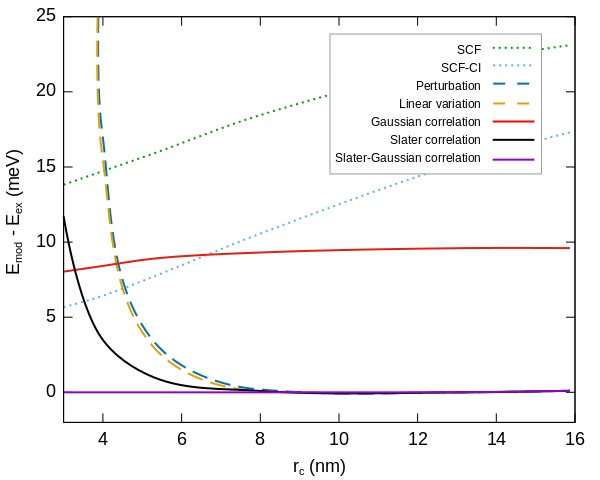
Figure 1: Energies, relative to the exact $E_{mod}-E_{ex}$, vs. confinement radius $r_{c}$, for the different approximate models of a two-dimensional exciton harmonically confined.

In figure 1 we collect the results of the different models particularized for CdSe, a typical semiconductor. In this case, the electron effective mass is isotropic, $m_{e}=0.12$, while the hole is highly anisotropic. Then, we should take the heavy hole in-plane effective mass $m_{h}=\frac{1}{\gamma_{1}+\gamma_{2}}\approx 0.15$. Finally, the dielectric constant is $\epsilon=9$.Woggon In the figure we represent the difference between the energy obtained by the different models and the exact energy vs. the confinement strength represented by the 2D harmonic oscillator confinement radius $r_{c}$. The confinement radius $r_{c}$ is related to the confining frequency $\omega$ by $\omega=\frac{2\hbar}{mr_{c}^{2}}$. Since electron and hole have different masses, in the above formula we consider $m$ to be the average $m=(m_{e}+m_{h})/2=0.135$.

Figure 1 neatly shows the different performance of the various approaches. The more sophisticated two parameter wave-function, that almost become a Slater function ($b\to 0$) in the low-confinement regime while has a larger contribution of the Gauss part in the strong confinement regime, yields an energy indistinguishable from the exact one in all confinement regimes. The one parameter Slater function does the same, except in the very strong confinement. Interestingly, the one parameter Gaussian function departs about 10 meV from the exact, independently of the confinement regime. It may be related to the fact that this particular system becomes a 2D harmonic oscillator if we remove the Coulomb term i.e., the Gaussian-like function is most suitable to describe the limit of highly strong confinement where the Coulomb contribution is negligible. The perturbation approach on the 2D hydrogen ground state eigenfunction has a performance similar to the one parameter Slater one, but deteriorates as the confinement get stronger. The addition of several s-orbitals to carry out a linear variation does not improve significantly the perturbation result. Finally, we can see that the (lower) accuracy of both SCF and SCF-CI changes depending on the confinement strength, showing then the poorest behavior amongst the different studied approaches.

The excellent behavior of the one parameter Slater function up to  5nm, which is well below typical nanoplatelets lateral dimensions,Woggon suggests it as the most suitable model for extensive yet reliable calculations. For this reason, in the following sections, all our models for excitons in 0D, quasi-1D and quasi-2D semiconductor quantum dots contain this correlation factor.

3 Models for quasi-2D, quasi-1D and 0D quantum dots

We present in Fig.2 the three systems we deal with. Building up appropriate simple one parameter variational models is the core of this paper. The goal is to reach models with simple analytical expressions for the kinetic energy (accounting for anisotropic mass) the normalization factor of the wave-function and the one-particle density (so that any one-body potential term may be calculated by means at most a 3D volume integral). In the following subsections we detail the different models for quasi-2D, quasi-1D and 0D quantum dots.

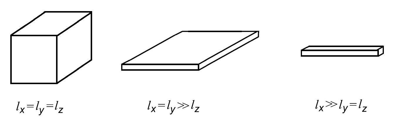
Figure 2: 0D, quasi-2D and quasi-1D quantum dots

3.1 Nanoplatelets in dielectric media: a quasi-2D system

The Hamiltonian of an exciton in a nanoplatelet reads,

$$\hat{H}=\sum_{e,h}\left[-\frac{\hbar^{2}}{2m_{\parallel,i}}\left(\frac{\partial^{2}}{\partial x^{2}}+\frac{\partial^{2}}{\partial y^{2}}\right)-\frac{\hbar^{2}}{2m_{z,i}}\frac{\partial^{2}}{\partial z^{2}}+V_{i}\right]$$

$$\hskip 19.91684pt+\;V_{c}(r_{e},r_{h})$$ (7)

where $V_{i}$ represent the sum of all possible single-particle potentials affecting particle $i$ and $V_{c}(r_{e},r_{h})$ represents the Coulomb interaction that may or not include dielectric effects. An infinite barrier is used to confine the exciton in the integration box. Please, note however that it does not mean that an infinite barrier is used to confine the exciton in the box, as the single particle $V_{i}$ potential may have a profile that mimics the band off-set between neighboring materials. At the end of the external material, where the wave function is null, we enclose the infinite wall, i.e., we assume the wave-function to be mathematically zero.

The exciton variational wave function is chosen to be a product of the electron and hole lowest-energy subband states and a Slater correlation factor.

$$\Psi(r_{e},r_{h})=N\cos kx_{e}\cos kx_{h}\cos ky_{e}\cos ky_{h}\cos\bar{k}z_{e}*$$

$$\hskip 71.13188pt*\cos\bar{k}z_{h}\;e^{-a\sqrt{(x_{e}-x_{h})^{2}+(y_{e}-y_{h})^{2}}\,}$$ (8)

where $N$ is the normalization factor, $k=\pi/L_{x}=\pi/L_{y}$ and $\bar{k}=\pi/L_{z}$. The form chosen for the wave-function gives the correct results for the ground state of the exciton in the limits of extremely high (small L) and negligible (large L) confinement. In the small-L limit the correlation factor becomes unity while in the large-L limit the correlation factor is the (2D) bulk-exciton ground-state wave function, and product of the electron and hole lowest-energy subband states are envelope functions which are slowly varying on the scale of the exciton. This wave-function is similar to that employed by BryantGarnett2 but have the advantage of using a Slater instead of a combination of Gaussian to mimic a Slater. We also provide a simple integration of the sixfold Coulomb integral, even in the presence of dielectric mismatch, only involving a twofold numerical integration.

The use of a Slater correlation factor has the additional advantage of being the unique correlation factor having a simple additive closed-form for the kinetic energy (see Appendix A for details):

$$\langle\Psi(r_{e},r_{h})|\hat{T}|\Psi(r_{e},r_{h})\rangle=\frac{\bar{k}^{2}}{2\mu_{z}}+\frac{k^{2}}{\mu_{\parallel}}+\frac{a^{2}}{2\mu_{\parallel}}$$ (9)

with $k=\pi/L_{x}=\pi/L_{y}$ and $\bar{k}=\pi/L_{z}$ and $a$ the variational parameter to be optimized.

3.1.1 The single-particle density

In this section we employ the labels 1 and 2 to refer to either particle and $L$ to refer to $L_{x}=L_{y}$. The single-particle density of particle ”1” reads,

$$\rho(r_{1})=\int|\Psi(r_{1},r_{2})|^{2}d^{3}r_{2}$$

$$=N^{2}\;\frac{L_{z}}{2}\cos^{2}\bar{k}z_{1}\cos^{2}kx_{1}\cos^{2}ky_{1}*$$

$$*\iint\displaylimits_{-L/2}^{\;\;L/2}\cos^{2}kx_{2}\cos^{2}ky_{2}\;e^{-2a\,\sqrt{(x_{2}-x_{1})^{2}+(y_{2}-y_{1})^{2}}}dx_{2}dy_{2}$$ (10)

After a rather long procedure, detailed in Appendix B, one can obtain the following closed-form for the single-particle density $\rho(r_{1})$:

$$\rho(r_{1})=N^{2}\;\frac{\pi\,L_{z}}{16}\;\cos^{2}\bar{k}z_{1}\;\cos^{2}kx_{1}\;\cos^{2}ky_{1}\;\;*$$

$$\hskip 28.45274pt*\left[\frac{1}{a^{2}}+\frac{a}{(a^{2}+k^{2})^{3/2}}\left(\cos 2kx_{1}+\cos 2ky_{1}\right)+\right.$$

$$\hskip 28.45274pt+\left.\frac{a}{(a^{2}+2k^{2})^{3/2}}\;\cos 2kx_{1}\cos 2ky_{1}\right]$$ (11)

The normalization factor, $N^{2}$ can now be obtained from the identity,

$$\int_{-L/2}^{L/2}\int_{-L/2}^{L/2}\int_{-L_{z}/2}^{L_{z}/2}\rho(x_{1},y_{1},z_{1})dx_{1}dy_{1}dz_{1}=1$$ (12)

Taking into account that $k=\pi/L$ and $\bar{k}=\pi/L_{z}$, we get:

$$N^{2}=\frac{128}{\pi\,L_{z}^{2}\,L^{2}}\;\left(\frac{1}{a^{2}}+\frac{a}{(a^{2}+k^{2})^{3/2}}+\frac{1}{4}\frac{a}{(a^{2}+2k^{2})^{3/2}}\right)^{-1}$$ (13)

3.1.2 Nanoplatelets with $L_{x}\neq L_{y}>>L_{z}$

For the sake of completeness we also enclose the case where the two in-plane dimensions are not alike. The calculation is similar to that with $L_{x}=L_{y}$. The kinetic energy is now:

$$\langle\Psi(r_{e},r_{h})|\hat{T}|\Psi(r_{e},r_{h})\rangle=\frac{k_{x}^{2}}{2\mu_{\parallel}}+\frac{k_{y}^{2}}{2\mu_{\parallel}}+\frac{k_{z}^{2}}{2\mu_{z}}+\frac{a^{2}}{2\mu_{\parallel}}$$ (14)

with $k_{x}=\pi/L_{x}$, $k_{y}=\pi/L_{y}$, $k_{z}=\pi/L_{z}$ and $a$ the variational parameter to be optimized.

The density reads:

$$\rho(r_{1})=N^{2}\;\frac{\pi\,L_{z}}{16}\;\cos^{2}k_{z}z_{1}\;\cos^{2}k_{x}x_{1}\;\cos^{2}k_{y}y_{1}\;*$$

$$*\left[\frac{1}{a^{2}}+\frac{a}{(a^{2}+k_{x}^{2})^{3/2}}\cos 2k_{x}x_{1}+\frac{a}{(a^{2}+k_{y}^{2})^{3/2}}\cos 2k_{y}y_{1}\right.$$

$$\left.\hskip 21.33955pt+\;\;\frac{a}{(a^{2}+k_{x}^{2}+k_{y}^{2})^{3/2}}\;\cos 2k_{x}x_{1}\cos 2k_{y}y_{1}\right]$$ (15)

with

$$N^{2}=\frac{128}{\pi\;L_{z}^{2}\,L_{x}\,L_{y}}\;\left[\frac{1}{a^{2}}+\frac{1}{2}\frac{a}{(a^{2}+k_{x}^{2})^{3/2}}+\right.$$

$$\hskip 21.33955pt\left.+\;\frac{1}{2}\frac{a}{(a^{2}+k_{y}^{2})^{3/2}}+\;\frac{1}{4}\frac{a}{(a^{2}+k_{x}^{2}+k_{y}^{2})^{3/2}}\right]^{-1}$$ (16)

It should be pointed out that the dimensions $L_{x}$ and $L_{y}$ should not be very different for a good performance of the model. If it was the case, in order to keep the accuracy, the correlation factor should be supplied with an additional variational parameter. Namely, $f(r_{eh})=\exp[-a\,\sqrt{(x_{e}-x_{h})^{2}+b\,(y_{e}-y_{h})^{2}}]$. A similar correlation factor has been proposed by Khramtsov et al.Khramtsov for the case of a 0D cuboid QD. However, the two-parameters model has not the simplicity of the single-parameter one so that no closed formulas for kinetic energy, density and normalization factors can be found. Then, the calculation becomes much heavier, unsuited for extensive calculations.

3.1.3 The polarized-Coulomb integral

We deal with the integral,

$$V_{c}=\int|\Psi({\bf r}_{e},{\bf r}_{h})|^{2}H_{c}\;d^{3}{\bf r}_{e}d^{3}{\bf r}_{h}$$ (17)

with $\Psi({\bf r}_{e},{\bf r}_{h})$ given in eq. (3.1) and $H_{c}$ represents the coulomb operator including the image charges originated in the dielectric mismatch of the nanoplatelet and the surrounding medium.Takagahara

$$H_{c}=-\sum_{n=-\infty}^{n=\infty}\frac{q_{n}}{\epsilon_{1}}\frac{1}{\sqrt{({\bf r}_{e,\parallel}-{\bf r}_{h,\parallel})^{2}+[z_{e}-(-1)^{n}\,z_{h}-n\,L_{z}]^{2}}}$$ (18)

where $q_{n}=(\frac{\epsilon_{1}-\epsilon_{2}}{\epsilon_{1}+\epsilon_{2}})^{|n|}$, $\epsilon_{1}$, $\epsilon_{2}$ are the nanoplatelet and surroundings dielectric constants, $L_{z}$ is the nanoplatelet height and ${\bf r}_{e,\parallel}$, ${\bf r}_{h,\parallel}$ the in-plane vector position of electron and hole. Please note that in the above equation (18) we disregard the image charges originated at the remote vertical nanoplatelet faces because their contribution is negligible and only account for those produced at the close horizontal ones located at a short $L_{z}/2$ distance. Then, integral (17) becomes,

$$V_{c}=N^{2}\;\iiiint\displaylimits_{-L/2}^{\;\;L/2}dx_{e}dx_{h}dy_{e}dy_{h}\cos^{2}kx_{e}\cos^{2}kx_{h}\;*$$

$$\hskip 14.22636pt*\;\cos^{2}ky_{e}\cos^{2}ky_{h}\;e^{-2a\sqrt{(x_{e}-x_{h})^{2}+(y_{e}-y_{h})^{2}}}*$$

$$\hskip 14.22636pt*\iint\displaylimits_{-L_{z}/2}^{\;\;\;L_{z}/2}dz_{e}dz_{h}\,H_{c}\,\cos^{2}\bar{k}z_{e}\cos^{2}\bar{k}z_{h}$$ (19)

First, we will turn the fourfold integral in $x_{e},x_{h},y_{e},y_{h}$ into a twofold one by means a double analytical integration. To this end we start by defining $kx_{e}=\xi_{e}$, $kx_{h}=\xi_{h}$ so that, since $k=\pi/L$, the original $[-L/2,L/2]$ integration limits become $[-\pi/2,\pi/2]$. Next, we define $\xi=\xi_{e}-\xi_{h}$ and $\xi^{\prime}=\xi_{e}+\xi_{h}$ so that,Romestain

$$\iint\displaylimits_{-L/2}^{\;\;L/2}dx_{e}dx_{h}\cos^{2}kx_{e}\cos^{2}kx_{h}\,f(|x_{e}-x_{h}|)=$$

$$\hskip 11.38092pt=\;\frac{1}{k^{2}}\iint\displaylimits_{-\pi/2}^{\;\;\pi/2}d\xi_{e}d\xi_{h}\cos^{2}\xi_{e}\cos^{2}\xi_{h}\,f(|\xi_{e}-\xi_{h}|)$$

$$\hskip 11.38092pt=\;\frac{1}{4k^{2}}\int_{0}^{\pi}d\xi\,[(\pi-\xi)(2+\cos 2\xi)+\frac{3}{2}\,\sin 2\xi]\,f(\xi)$$ (20)

For details on the last step in (3.1.3) see Appendix D. We do the same tranformation to the $y$ coordinates and refer either new coordinate to as $\xi_{x}$ and $\xi_{y}$. Then, with the notation $g(\xi)=(\pi-\xi)(2+\cos 2\xi)+\frac{3}{2}\,\sin 2\xi$, the Coulomb integral (3.1.3) can be rewritten as:

$$V_{c}=\frac{N^{2}}{16}\frac{1}{k^{4}}\iint\displaylimits_{0}^{\;\;\pi}g(\xi_{x})\,g(\xi_{y})\exp[-\frac{2a}{k}\sqrt{\xi_{x}^{2}+\xi_{y}^{2}}]\,*\,{\bf I}_{2}$$ (21)

with

$${\bf I}_{2}=\iint\displaylimits_{-L_{z}/2}^{\;\;L_{z}/2}dz_{e}dz_{h}\,H_{c}(\xi_{x},\xi_{y},z_{e},z_{h})\,\cos^{2}\bar{k}z_{e}\cos^{2}\bar{k}z_{h}$$

$$=\;\frac{1}{\bar{k}^{2}}\iint\displaylimits_{-\pi/2}^{\;\;\pi/2}d\xi_{ze}d\xi_{zh}\,\,H_{c}(\xi_{x},\xi_{y},\xi_{ze},\xi_{zh})\,\,\cos^{2}\xi_{ze}\cos^{2}\xi_{zh}$$ (22)

where now the n-th $H_{c}$ term reads:

$$\frac{q_{n}}{\epsilon_{1}}\,\frac{1}{\sqrt{(1/k^{2})(\xi_{x}^{2}+\xi_{y}^{2})+(1/\bar{k}^{2})\,[\xi_{ze}-(-1)^{n}\,\xi_{zh}-n\pi]^{2}}}.$$ (23)

The integral ${\bf I}_{2}$ cannot be calculated analytically. We then calculate ${\bf I}_{2}$ semi-analytically. To this end we consider that

$$\int_{a}^{b}f(x)g(x)dx=\sum_{i=1}^{N-1}g(a+(i-1/2)\Delta)\;\int_{a+(i-1)\Delta}^{a+i\,\Delta}f(x)dx$$ (24)

where $g(x)$ is a smooth function while $f(x)$ may have regions with sharp gradients. This strategy is in the core of the envelope function $k\cdot p$ model widely employed to describe semiconductor heterostructures and quantum dots.Bastard

In our case the smooth function is the product of cosines. Then, should we withdraw this product the resulting integral has primitive:

$$P(\xi_{ze},\xi_{zh})=\iint\frac{d\xi_{ze}d\xi_{zh}}{\sqrt{a^{2}+[\xi_{ze}-(-1)^{n}\,\xi_{zh}-n\pi]^{2}}}\;=$$

$$\hskip 2.84544pt=\;(-1)^{n}\left\{\sqrt{a^{2}+(n\pi-\xi_{ze}+(-1)^{n}\,\xi_{zh})^{2}}\right.+$$

$$\hskip 14.22636pt+\;(-1)^{n}\,\xi_{zh}\,\log\left[-n\pi+\xi_{ze}-(-1)^{n}\,\xi_{zh}+\right.$$

$$\hskip 56.9055pt\left.+\;\sqrt{a^{2}+(n\pi-\xi_{ze}+(-1)^{n}\,\xi_{zh})^{2}}\right]$$

$$\hskip 14.22636pt+\;(\xi_{ze}-n\pi)\,\log\left[n\pi-\xi_{ze}+(-1)^{n}\,\xi_{zh}+\right.$$

$$\hskip 56.9055pt\left.\left.+\;\sqrt{a^{2}+(n\pi-\xi_{ze}+(-1)^{n}\,\xi_{zh})^{2}}\right]\right\}$$ (25)

Then, we divide symmetrically the interval $[-\pi/2,\pi/2]$ in a pair number $N$ of subintervals and in each subinterval we replace the smooth function $g(x)$ by its value at the center of it $g(a+(i-1/2)\Delta)$ and write the integral with limits $[a,b]$ as a sum of $N$ analytical functions. In our case, after labeling as $\xi_{ze}^{(i)},\xi_{ze}^{(f)},\xi_{zh}^{(i)},\xi_{zh}^{(f)}$ the limits of the subinterval, the result of the integral in it is:

$$\cos^{2}[\frac{1}{2}(\xi_{ze}^{(f)}+\xi_{ze}^{(i)})]\cos^{2}[\frac{1}{2}(\xi_{zh}^{(f)}+\xi_{zh}^{(i)})]\;*$$

$$\hskip 28.45274pt*\;\left[P(\xi_{ze}^{(f)},\xi_{zh}^{(f)})+P(\xi_{ze}^{(i)},\xi_{zh}^{(i)})\right.-$$

$$\hskip 56.9055pt\left.-\,P(\xi_{ze}^{(f)},\xi_{zh}^{(i)})-P(\xi_{ze}^{(i)},\xi_{zh}^{(f)})\right].$$ (26)

The result of integration in $z$ is then a sum of terms only dependent on $\xi_{x},\xi_{y}$ that we refer to as $Z(\xi_{x},\xi_{y})$. The usefulness of the application of (24) in our case is that $Z(\xi_{x},\xi_{y})$ and then the Coulomb integral is highly convergent with the number $N$ of subintervals.Movilla

From the above algebra, the sixfold Coulomb integral turns into the following numerical twofold one:

$$V_{c}=\frac{N^{2}}{16}\frac{1}{k^{4}}\iint\displaylimits_{0}^{\;\;\;\;\pi}d\xi_{x}d\xi_{y}\,g(\xi_{x})g(\xi_{y})Z(\xi_{x},\xi_{y})e^{-\frac{2a}{k}\sqrt{\xi_{x}^{2}+\xi_{y}^{2}}}$$ (27)

In the case of a rectangular nanoplatelet we proceed in a similar way, just taking into account that now instead of a unique $k=\pi/L$ we have $k_{x}=\pi/L_{x}$ and $k_{y}=\pi/L_{y}$.

3.2 Long nanorods: a quasi-1D system

The exciton variational wave function is also chosen to be a product of the electron and hole lowest-energy subband states and a Slater correlation factor.

$$\Psi(r_{e},r_{h})=N\cos kx_{e}\cos kx_{h}\cos\bar{k}y_{e}\cos\bar{k}y_{h}\;*$$

$$\hskip 85.35826pt\cos\bar{k}z_{e}\cos\bar{k}z_{h}\;e^{-a|x_{e}-x_{h}|}$$ (28)

Where $N$ is the normalization factor, $k=\pi/L_{x}$ and $\bar{k}=\pi/L_{y}=\pi/L_{z}$. This wave-function also gives the correct results for the ground state of the exciton in the limits of extremely high (small $L_{x}$) and negligible (large $L_{x}$) confinement.

As above, the use of a Slater correlation factor has the advantage of having a simple additive closed-form for the kinetic energy (see Appendix A for details):

$$\langle\Psi(r_{e},r_{h})|\hat{T}|\Psi(r_{e},r_{h})\rangle=\frac{\bar{k}^{2}}{2\mu_{z}}+\frac{\bar{k}^{2}}{2\mu_{\parallel}}+\frac{k^{2}}{2\mu_{\parallel}}+\frac{a^{2}}{2\mu_{\parallel}}$$ (29)

with $k=\pi/L_{x}$ and $\bar{k}=\pi/L_{y}=\pi/L_{z}$ and $a$ the variational parameter to be optimized.

3.2.1 The single-particle density

In this section we also employ the labels 1 and 2 to refer to either particle and $L$ to refer to $L_{y}=L_{z}$. In Appendix C we enclose the value of the integrals employed to derive the kinetic energy, density and norm of the above wave-function. The single-particle density of particle ”1” reads,

$$\rho(r_{1}) = \int|\Psi(r_{1},r_{2})|^{2}d^{3}r_{2}=N^{2}\;(\frac{L}{2})^{2}\cos^{2}\bar{k}y_{1}\cos^{2}\bar{k}z_{1}\;*$$ (30)

$$* \int_{-L_{x}/2}^{L_{x}/2}\cos^{2}kx_{1}\cos^{2}kx_{2}e^{-2a\,|x_{2}-x_{1}|}\;dx_{2}$$

Since (see Appendix C)

$$\int_{-L_{x}/2}^{L_{x}/2}\cos^{2}kx_{2}\;e^{-2a\,|x_{2}-x_{1}|}\;dx_{2}\;=$$

$$\hskip 85.35826pt=\;\frac{1}{2a}+\frac{a}{2\,(a^{2}+k^{2})}\cos 2kx_{1}$$ (31)

the single-particle density results:

$$\rho(r_{1})=N^{2}\;(\frac{L}{2})^{2}\;\left[\frac{1}{2a}+\frac{a}{2\,(a^{2}+k^{2})}\cos 2kx_{1}\right]\;*$$

$$\hskip 85.35826pt*\;\cos^{2}\bar{k}y_{1}\;\cos^{2}\bar{k}z_{1}\;\cos^{2}kx_{1}$$ (32)

Finally, by integrating $\rho(r_{1})$, we get the norm:

$$N^{2}=(\frac{2}{L})^{4}\,(\frac{2}{L_{x}})\,\frac{8a\,(a^{2}+k^{2})}{6a^{2}+4k^{2}}$$ (33)

3.2.2 The bare-Coulomb integral

We show here that the sixfold integral,

$$V_{c}=\int\frac{|\Psi({\bf r}_{e},{\bf r}_{h})|^{2}}{\epsilon\,|{\bf r}_{e}-{\bf r}_{h}|}\;d^{3}{\bf r}_{e}d^{3}{\bf r}_{h}$$ (34)

where $\Psi({\bf r}_{e},{\bf r}_{h})$ is given in eq. (3.2), can be reduced up to a one-coordinate numerical integration. To this end we first turn the sixfold integral in $x_{e},x_{h},y_{e},y_{h},z_{e},z_{h}$ into a threefold one by using the set of variables $\xi_{x}$, $\xi^{\prime}_{x}$,$\xi_{y}$, $\xi^{\prime}_{y}$,$\xi_{z}$, $\xi^{\prime}_{z}$, with $\xi_{x}=k(x_{e}-x_{h})$, $\xi^{\prime}_{x}=k(x_{e}+x_{h})$ $\dots$ $\xi^{\prime}_{z}={\bar{k}}(z_{e}+z_{h})$, and carry out analytical integrations over $\xi^{\prime}_{i}\,$Romestain yielding (see Appendix D for details),

$$V_{c}=\frac{N^{2}}{2^{6}}\frac{1}{k^{2}\,\bar{k}^{4}}\frac{1}{\epsilon}\iiint\displaylimits_{0}^{\hskip 8.5359pt\pi}d\xi_{x}d\xi_{y}d\xi_{z}\,g(\xi_{x})g(\xi_{y})g(\xi_{z})\;*$$

$$\hskip 71.13188pt*\;e^{-\frac{2a}{k}\,\xi_{x}}\;\frac{\bar{k}}{\sqrt{(\bar{k}/k)^{2}\,\xi_{x}^{2}+\xi_{y}^{2}+\xi_{z}^{2}}}$$ (35)

with $g(\xi_{i})=(\pi-\xi_{i})(2+\cos 2\xi_{i})+\frac{3}{2}\,\sin 2\xi_{i}$.

Now, we may numerically integrate this threefold integral. Alternatively, we can consider the primitive $P(\xi_{y},\xi_{z})$ of the next integral,

$$P(\xi_{y},\xi_{z})=\iint\frac{d\xi_{y}d\xi_{z}}{\sqrt{a^{2}+\xi_{y}^{2}+\xi_{z}^{2}}}=-\xi_{y}+a\,\arctan\frac{\xi_{y}}{a}\;-$$

$$-a\,\arctan\frac{\xi_{y}\xi_{z}}{a\,\sqrt{a^{2}+\xi_{y}^{2}+\xi_{z}^{2}}}+\xi_{z}\log(\xi_{y}+\sqrt{a^{2}+\xi_{y}^{2}+\xi_{z}^{2}}\;)\;+$$

$$+\xi_{y}\log(\xi_{z}+\sqrt{a^{2}+\xi_{y}^{2}+\xi_{z}^{2}}\;)$$ (36)

where $a=\frac{\bar{k}}{k}\,\xi_{x}$, that can also be written as,

$$P(\xi_{y},\xi_{z})=\iint\frac{d\xi_{z}d\xi_{y}}{\sqrt{a^{2}+\xi_{y}^{2}+\xi_{z}^{2}}}=-\xi_{z}+a\,\arctan\frac{\xi_{z}}{a}\;-$$

$$-a\,\arctan\frac{\xi_{y}\xi_{z}}{a\,\sqrt{a^{2}+\xi_{y}^{2}+\xi_{z}^{2}}}+\xi_{z}\log(\xi_{y}+\sqrt{a^{2}+\xi_{y}^{2}+\xi_{z}^{2}}\;)\;+$$

$$+\xi_{y}\log(\xi_{z}+\sqrt{a^{2}+\xi_{y}^{2}+\xi_{z}^{2}}\;).$$ (37)

Please note that for any square interval of limits $\{[\xi_{y}^{(i)},\xi_{y}^{(f)}]$, $[\xi_{z}^{(i)},\xi_{z}^{(f)}]\}$, the definite integral $[P(\xi_{y}^{(f)},\xi_{z}^{(f)})+P(\xi_{y}^{(i)},\xi_{z}^{(i)})-P(\xi_{y}^{(f)},\xi_{z}^{(i)})-P(\xi_{y}^{(i)},\xi_{z}^{(f)})]$ is the same, irrespectively of using $P(\xi_{y},\xi_{z})$ according to eq. (3.2.2) or eq. (3.2.2).

This result allows to perform the integral,

$$Z(\xi_{x})=\iint\displaylimits_{0}^{\;\;\;\;\;\;\pi}d\xi_{y}d\xi_{z}\,g(\xi_{y})\,g(\xi_{z})\,\frac{\bar{k}}{\sqrt{(\bar{k}/k)^{2}\,\xi_{x}^{2}+\xi_{y}^{2}+\xi_{z}^{2}}}$$ (38)

as a sum of terms like:

$$g[\frac{1}{2}(\xi_{z}^{(i)}+\xi_{z}^{(f)})]\,g[\frac{1}{2}(\xi_{y}^{(i)}+\xi_{y}^{(f)})]\;[P(\xi_{y}^{(f)},\xi_{z}^{(f)})+$$

$$\hskip 21.33955pt+\;P(\xi_{y}^{(i)},\xi_{z}^{(i)})-P(\xi_{y}^{(f)},\xi_{z}^{(i)})-P(\xi_{y}^{(i)},\xi_{z}^{(f)})].$$ (39)

Finally, we numerically obtain the bare Coulomb term by carrying out the one-coordinate integral:

$$\int_{0}^{\pi}d\xi_{x}\,g(\xi_{x})\,Z(\xi_{x})\;e^{-\frac{2a}{k}\,\xi_{x}}.$$ (40)

3.3 Cubic quantum dots: a 0D system

As in the above sections, the exciton variational wave function is chosen to be a product of the electron and hole lowest-energy subband states and a Slater correlation factor.

$$\Psi(r_{e},r_{h})=N\cos kx_{e}\cos kx_{h}\cos ky_{e}\cos ky_{h}\cos kz_{e}\;*$$

$$\hskip 28.45274pt*\,\cos kz_{h}\;e^{-a\sqrt{(x_{e}-x_{h})^{2}+(y_{e}-y_{h})^{2}++(z_{e}-z_{h})^{2}}}$$ (41)

This variational wave-function has been previously employed by Romestain and Fishman.Romestain We follow similar techniques as those employed in the previous sections to derive closed form of the kinetic energy, single-particle density and the normalization factor. We present next the model for cubic QDs. The extension to cuboid QDs is straightforward with the help of integrals in Appendix C.

3.3.1 The single-particle density

The single-particle density of particle ”1” reads,

$$\rho(r_{1})=\int|\Psi(r_{1},r_{2})|^{2}d^{3}r_{2}=N^{2}\,\cos^{2}kx_{1}\cos^{2}ky_{1}\cos^{2}kz_{1}*$$

$$\hskip 28.45274pt*\;\iiint\displaylimits_{-L/2}^{\;\;\;L/2}dx_{2}\,dy_{2}\,dz_{2}\,\cos^{2}kx_{2}\cos^{2}ky_{2}\cos^{2}kz_{2}\;*$$

$$\hskip 56.9055pt*\;e^{-2a\,\sqrt{(x_{2}-x_{1})^{2}+(y_{2}-y_{1})^{2}+(z_{2}-z_{1})^{2}}}$$ (42)

We obtain in Appendix B the following closed-form for the single-particle density:

$$\rho(r_{1})=N^{2}\,\frac{\pi}{8}\;\cos^{2}kx_{1}\;\cos^{2}ky_{1}\;\cos^{2}kz_{1}\;*$$

$$\hskip 14.22636pt*\;\left\{\frac{1}{a^{3}}+\frac{a}{(a^{2}+k^{2})^{2}}\left(\cos 2kx_{1}+\cos 2ky_{1}+\cos 2kz_{1}\right)\right.$$

$$\hskip 28.45274pt+\frac{a}{(a^{2}+2k^{2})^{2}}\left[\cos 2kx_{1}\,\cos 2ky_{1}\;+\right.$$

$$\hskip 71.13188pt\left.+\cos 2kx_{1}\,\cos 2kz_{1}+\,\cos 2ky_{1}\,\cos 2kz_{1}\right]$$

$$\hskip 28.45274pt\left.+\frac{a}{(a^{2}+3k^{2})^{2}}\;\cos 2kx_{1}\,\cos 2ky_{1}\,\cos 2kz_{1}\right\}$$ (43)

The integration of $\rho(r_{1})$ from $-L/2$ up to $L/2$ in all three coordinates should yield the unity. Then, since $k=\pi/L$, we get the norm:

$$N^{2}=\frac{512\,a^{3}}{\pi\,L^{3}}\;\left(8+\frac{12}{(1+(\frac{k}{a})^{2})^{2}}\,+\right.$$

$$\hskip 56.9055pt\left.+\frac{6}{(1+2\,(\frac{k}{a})^{2})^{2}}+\frac{1}{(1+3\,(\frac{k}{a})^{2})^{2}}\right)^{-1}$$ (44)

In order to extend the previous model to cuboid QDs with edges of different length we would just make use of the last two eqs. in Appendix C.2. All the same, as pointed out above, if the lengths of the cuboid QD are not similar, the use of a single variational parameter model may not be enough to reach the same accuracy than that reached for cubic QDs. In order to keep the accuracy, the correlation factor should be supplied with additional variational parameters. Namely, $f(r_{eh})=\exp[-a\,\sqrt{(x_{e}-x_{h})^{2}+b\,(y_{e}-y_{h})^{2}+c\,(z_{e}-z_{h})^{2}}]$. However, the three-parameters model has not the simplicity of the single-parameter one: no closed formulas for kinetic energy, density and normalization factors can be found in this case and, therefore, the calculation becomes much heavier, unable for extensive calculations.

4 Summary

We derive closed-form formulas for the normalization factor, single-particle density and expectation value of the kinetic energy for simple correlated exciton wave-functions chosen to be a product of the electron and hole lowest-energy subband states times a Slater correlation factor suited to describe 0D, quasi-1D and quasi-2D systems. We also provide fast integration procedures for the Coulomb integral in typical quasi-2D nanoplatelets including polarization of the Coulomb interaction, and for the bare-Coulomb integral in quasi-1D long nanorods. For nanoplatelets, the original sixfold integral is reduced to a twofold numerical integral, while a one-coordinate numerical integration is required for quasi-1D systems. This theoretical baggage should enable accurate yet reliable simulations of electronic structure in strongly correlated exciton systems of current interest.

Appendix A Deriving the expectation value of the kinetic energy for the different models

A.1 Cuboid QD and nanoplatelet

The normalized wave-function for these models is $\Psi=\Phi({\bf r}_{e},{\bf r}_{h})\chi(r_{eh})$ with $\Phi({\bf r}_{e},{\bf r}_{h})=\phi_{e}({\bf r}_{e})\,\phi_{h}({\bf r}_{h})$ and $\chi(r_{eh})$ $=\exp[-a\,r_{eh}]$. In the 0D model $r_{eh}$ is three-dimensional i.e. $r_{eh}=\sqrt{(x_{e}-x_{h})^{2}+(y_{e}-y_{h})^{2}+(z_{e}-z_{h})^{2}}$ while the the quasi-2D model it is two-dimensional i.e., $r_{eh}=\sqrt{(x_{e}-x_{h})^{2}+(y_{e}-y_{h})^{2}}$.

The most general kinetic energy operator reads,

$$\hat{T}=\sum_{i=e,h}\;\sum_{a=x,y,z}-\frac{1}{2m_{ia}}\frac{\partial^{2}}{\partial a_{i}^{2}}$$ (45)

In order to simplify the notation we define $D=\frac{\partial}{\partial a_{i}}$ and $w=\langle\Psi|D^{2}|\Psi\rangle$. We have,

$$D^{2}(F\,G)=(D^{2}\,F)\,G+2\,(DF)(DG)+F\,(D^{2}G)$$ (46)

$$w=\langle\Phi\;\chi^{2}|D^{2}\Phi\rangle+\langle\Phi^{2}\,\chi|D^{2}\chi\rangle+2A$$ (47)

with,

$$A=\langle\Phi\,\chi|(D\Phi)(D\chi)\rangle=\frac{1}{4}\,\langle(D\Phi^{2})(D\chi^{2})\rangle.$$ (48)

Since $\Phi=0$ at the integration limit, after integration by parts,

$$A=-\frac{1}{4}\;\langle\Phi^{2}|(D^{2}\chi^{2})\rangle.$$ (49)

Finally,

$$W=\langle\Psi|\hat{T}|\Psi\rangle=\langle\Phi\,\chi^{2}|\hat{T}|\Phi\rangle+\langle\Phi^{2}|\chi\,(\hat{T}\chi)-\frac{1}{2}(\hat{T}\chi^{2})\rangle.$$ (50)

We have that $\hat{T}\Phi=E\Phi$. Since $\frac{1}{m_{e}}+\frac{1}{m_{h}}=\frac{1}{\mu}$, then

$$E=\frac{k_{x}^{2}}{2\mu_{x}}+\frac{k_{y}^{2}}{2\mu_{y}}+\frac{k_{z}^{2}}{2\mu_{z}}$$ (51)

In the case of a cubic 0D QD with isotropic mass $E=\frac{3k^{2}}{2\mu}$ while $E=\frac{1}{2\mu}\,(k_{x}^{2}+k_{y}^{2}+k_{z}^{2})$ for a cuboid QD. For a platelet with anisotropic mass $E=\frac{k^{2}}{\mu_{\parallel}}+\frac{k_{z}}{2\mu_{z}}$.

We calculate next the second integral in eq. (50) for the case of an isotropic QD. To this end we use center-of-mass and relative motion coordinates: ${\bf R}=(m_{e}{\bf r}_{e}+m_{h}{\bf r}_{h})/M$, ${\bf r}={\bf r}_{e}-{\bf r}_{h}$. We have,

$$\hat{T}=\frac{P^{2}}{2M}+\frac{p^{2}}{2\mu}=\hat{T}_{R}+\hat{T}_{r}$$ (52)

Since $\chi=\exp[-ar]$, $\hat{T}\,\chi=\hat{T}_{r}\,\chi=-\frac{1}{2}\frac{1}{r^{2}}\frac{d}{dr}(r^{2}\frac{d}{dr})\;\chi$. Then,

$$\chi\,\hat{T}\,\chi-\frac{1}{2}\,\hat{T}\,\chi^{2}=\chi\,\hat{T}_{r}\,\chi-\frac{1}{2}\,\hat{T}_{r}\,\chi^{2}=\frac{a^{2}}{2\mu}\;\chi^{2}$$ (53)

and

$$W=\frac{3\,k^{2}}{2\,\mu}+\frac{a^{2}}{2\,\mu}$$ (54)

In the case of a nanoplatelet the correlation factor is two-dimensional ($r_{eh}=\sqrt{(x_{e}-x_{h})^{2}+(y_{e}-y_{h})^{2}}\;$). We follow now similar steps as above but instead of spherical we use polar $(r,\theta,z)$ coordinates. In this case,

$$\hat{T}_{r}=-\frac{1}{2\mu_{\parallel}}\;(\frac{\partial^{2}}{\partial r^{2}}+\frac{1}{r}\frac{\partial}{\partial r})$$ (55)

and

$$\chi\,\hat{T}\,\chi-\frac{1}{2}\,\hat{T}\,\chi^{2}=\chi\,\hat{T}_{r}\,\chi-\frac{1}{2}\,\hat{T}_{r}\,\chi^{2}=\frac{a^{2}}{2\mu_{\parallel}}\;\chi^{2}$$ (56)

So that finally,

$$W=\frac{k^{2}}{\mu_{\parallel}}+\frac{k_{z}^{2}}{2\,\mu_{z}}+\frac{a^{2}}{2\,\mu_{\parallel}}.$$ (57)

A.2 Long nanorod

The wave-function in this case, eq. (3.2), is:

$$\Psi(r_{e},r_{h})=N\cos kx_{e}\cos kx_{h}\cos\bar{k}y_{e}\cos\bar{k}y_{h}\;*$$

$$\hskip 85.35826pt*\;\cos\bar{k}z_{e}\cos\bar{k}z_{h}\;e^{-a|x_{e}-x_{h}|}$$

It is immediate to find that,

$$\frac{\langle\Psi|\hat{T}_{y}|\Psi\rangle}{\langle\Psi|\Psi\rangle}=\frac{\bar{k}^{2}}{2\mu_{\parallel}}$$ (58)

with $\hat{T}_{y}=-\frac{1}{2m_{e,\parallel}}\,\frac{\partial^{2}}{\partial y_{e}^{2}}\,-\frac{1}{2m_{h,\parallel}}\,\frac{\partial^{2}}{\partial y_{h}^{2}}$ and $\frac{1}{m_{e}}+\frac{1}{m_{h}}=\frac{1}{\mu}$.

Similarly we find that,

$$\frac{\langle\Psi|\hat{T}_{z}|\Psi\rangle}{\langle\Psi|\Psi\rangle}=\frac{\bar{k}^{2}}{2\mu_{z}}$$ (59)

For the long edge, with $\hat{T}_{x}=-\frac{1}{2m_{e,\parallel}}\,\frac{\partial^{2}}{\partial x_{e}^{2}}\,-\frac{1}{2m_{h,\parallel}}\,\frac{\partial^{2}}{\partial x_{h}^{2}}$, $\langle\Psi|\Psi\rangle=1$, we have,

$$\frac{\langle\Psi|\hat{T}_{x}|\Psi\rangle}{\langle\Psi|\Psi\rangle}=N^{2}\,\int_{-\frac{L}{2}}^{\frac{L}{2}}dy_{e}\,\cos^{2}\bar{k}y_{e}\,\int_{-\frac{L}{2}}^{\frac{L}{2}}dy_{h}\,\cos^{2}\bar{k}y_{h}\,*$$

$$\hskip 14.22636pt*\;\int_{-\frac{L}{2}}^{\frac{L}{2}}dz_{e}\,\cos^{2}\bar{k}z_{e}\,\int_{-\frac{L}{2}}^{\frac{L}{2}}dz_{h}\,\cos^{2}\bar{k}z_{h}\;*$$

$$\hskip 14.22636pt*\iint\displaylimits_{-\frac{L_{x}}{2}}^{\;\;\;\;\frac{L_{x}}{2}}dx_{e}dx_{h}\cos kx_{e}\,\cos kx_{h}\;e^{-a\,|x_{e}-x_{h}|}\;*$$

$$\hskip 71.13188pt\hat{T}_{x}\,\cos kx_{e}\,\cos kx_{h}\exp[-a\,|x_{e}-x_{h}|]$$

$$=N^{2}\,(\frac{L}{2})^{4}\;({\bf I}_{1}+{\bf I}_{2})$$ (60)

Since

$$\frac{d^{2}}{dx_{e}^{2}}\left(\cos kx_{e}\,e^{-a\,|x_{h}-x_{e}|}\right)=e^{-a\,|x_{h}-x_{e}|}\,*$$

$$\hskip 28.45274pt*\,[(a^{2}-k^{2})\,\cos kx_{e}+2ak\,\frac{|x_{h}-x_{e}|}{x_{h}-x_{e}}\,\sin kx_{e}$$

$$\hskip 99.58464pt-2a\,\cos kx_{e}\,\delta(x_{h}-x_{e})]$$ (61)

The integral ${\bf I}_{1}$ becomes split into a sum of three integrals, ${\bf I}_{1}={\bf I}_{11}+{\bf I}_{12}+{\bf I}_{13}$, where (see Appendix C.1 for the employed definite integrals),

$${\bf I}_{11} = -\frac{a^{2}-k^{2}}{2m_{e}}\,\int_{-\frac{L_{x}}{2}}^{\frac{L_{x}}{2}}dx_{e}\,\cos^{2}k_{e}\;*$$ (62)

$$\hskip 42.67912pt*\;\int_{-\infty}^{\infty}dx_{h}\,\cos kx_{h}\exp[-2a\,|x_{h}-x_{e}|]$$

$$= -\frac{a^{2}-k^{2}}{2m_{e}}\,\int_{-\frac{L_{x}}{2}}^{\frac{L_{x}}{2}}dx_{e}\,\cos^{2}k_{e}\;\left(\frac{1}{2a}+\frac{a\,\cos 2kx_{e}}{2\,(a^{2}+k^{2})}\right)$$

$$= -\frac{a^{2}-k^{2}}{2m_{e}}\,\left\{\frac{1}{2a}\,\int_{-\frac{L_{x}}{2}}^{\frac{L_{x}}{2}}dx_{e}\,\cos^{2}k_{e}\;\right.+$$

$$\hskip 28.45274pt\left.+\,\frac{a}{2\,(a^{2}+k^{2})}\,\int_{-\frac{L_{x}}{2}}^{\frac{L_{x}}{2}}dx_{e}\,\cos^{2}kx_{e}\,\cos 2kx_{e}\right\}$$

$$= -\frac{a^{2}-k^{2}}{2m_{e}}\,\frac{L_{x}}{2}\;\left(\frac{1}{2a}+\frac{a/4}{a^{2}+k^{2}}\right)$$

$${\bf I}_{12} = -\frac{a\,k}{m_{e}}\;\int_{-\frac{L_{x}}{2}}^{\frac{L_{x}}{2}}dx_{h}\,\cos^{2}kx_{h}\,*$$ (63)

$$* \int_{-\infty}^{\infty}dx_{e}\,\cos kx_{e}\,\sin kx_{e}\,\frac{|x_{h}-x_{e}|}{x_{e}-x_{h}}\;e^{-2a|x_{h}-x_{e}|}$$

Since (see Appendix C.1),

$$\int_{-\infty}^{\infty}d\bar{x}_{e}\,\sin 2k(\bar{x}_{e}+x_{h})\frac{|\bar{x}_{e}|}{\bar{x}_{e}}\;\exp[-2a|\bar{x}_{e}|]=$$

$$\hskip 99.58464pt=\;\;\frac{k}{a^{2}+k^{2}}\;\cos 2kx_{h}$$ (64)

then,

$${\bf I}_{12} = -\frac{a\,k}{m_{e}}\;\frac{1}{2}\,\frac{k}{a^{2}+k^{2}}\;\int_{-\frac{L_{x}}{2}}^{\frac{L_{x}}{2}}dx_{h}\,\cos^{2}kx_{h}\,\cos 2kx_{h}$$ (65)

$$= -\frac{a\,k^{2}}{2m_{e}}\,\frac{1}{a^{2}+k^{2}}\,\frac{L_{x}}{4}.$$

Now we integrate ${\bf I}_{13}$:

$${\bf I}_{13} = \frac{a}{m_{e}}\,\int\displaylimits_{-\frac{L_{x}}{2}}^{\;\;\;\frac{L_{x}}{2}}dx_{e}\,dx_{h}\,\;\delta(x_{h}-x_{e})\;\cos^{2}kx_{e}\;*$$ (66)

$$\hskip 85.35826pt*\;\cos^{2}kx_{h}\;e^{-2a|x_{h}-x_{e}|}$$

$$= \frac{a}{m_{e}}\;\int_{-\frac{L_{x}}{2}}^{\frac{L_{x}}{2}}dx_{e}\,\cos^{2}kx_{e}\;*$$

$$*\;\int_{-\infty}^{\infty}dx_{h}\,\cos^{2}kx_{h}\;\exp[-2a|x_{h}-x_{e}|]\;\delta(x_{h}-x_{e})$$

$$= \frac{a}{m_{e}}\;\int_{-\frac{L_{x}}{2}}^{\frac{L_{x}}{2}}dx_{e}\,\cos^{2}kx_{e}\,\cos^{2}kx_{e}$$

$$= \frac{3aL_{x}}{8m_{e}}.$$

From eqs. (62), (65) and (66), we obtain ${\bf I}_{1}$:

$${\bf I}_{1}=\frac{L_{x}}{4\,a}\left(\frac{k^{2}}{2m_{e}}+\frac{3}{2}\frac{a^{2}}{2m_{e}}\right)$$ (67)

The integral ${\bf I}_{2}$ in eq. (A.2) is like ${\bf I}_{1}$ replacing $e$ by $h$. From ${\bf I}_{1}$ and ${\bf I}_{2}$, with $\frac{1}{m_{e}}+\frac{1}{m_{h}}=\frac{1}{\mu}$, we obtain ${\bf I}_{1}+{\bf I}_{2}=\frac{L_{x}}{4a}\left(\frac{k^{2}}{2\mu_{\parallel}}+\frac{3}{2}\frac{a^{2}}{2\mu_{\parallel}}\right)$, so that:

$$\frac{\langle\Psi|\hat{T}_{x}|\Psi\rangle}{\langle\Psi|\Psi\rangle} = N^{2}\,(\frac{L}{2})^{4}\;({\bf I}_{1}+{\bf I}_{2})$$ (68)

$$= \frac{1}{2\mu_{\parallel}}\;(a^{2}+k^{2})$$

Then,

$$\frac{\langle\Psi|\hat{T}|\Psi\rangle}{\langle\Psi|\Psi\rangle}=\frac{\bar{k}^{2}}{2\mu_{\parallel}}+\frac{\bar{k}^{2}}{2\mu_{z}}+\frac{k^{2}}{2\mu_{\parallel}}+\frac{a^{2}}{2\mu_{\parallel}}.$$ (69)

Appendix B The single-particle density

B.1 The single-particle density of quasi-2D systems

We employ the labels 1 and 2 to refer to either particle and $L$ to refer to $L_{x}=L_{y}$. The single-particle density of particle ”1” reads,

$$\rho(r_{1})=\int|\Psi(r_{1},r_{2})|^{2}d^{3}r_{2}$$

$$=N^{2}\;\frac{L_{z}}{2}\cos^{2}\bar{k}z_{1}\cos^{2}kx_{1}\cos^{2}ky_{1}*$$

$$*\iint\displaylimits_{-L/2}^{\;\;L/2}\cos^{2}kx_{2}\cos^{2}ky_{2}\;e^{-2a\,\sqrt{(x_{2}-x_{1})^{2}+(y_{2}-y_{1})^{2}}}dx_{2}dy_{2}$$

$$=N^{2}\;\frac{L_{z}}{2}\cos^{2}\bar{k}z_{1}\cos^{2}kx_{1}\cos^{2}ky_{1}*\bf I$$ (70)

The identity $2\cos^{2}A=1+\cos 2A$ removes the squares in the cosines of integral $\bf I$. Next, we carry out the following change of variables: $x_{2}-x_{1}=\bar{x}_{2}$, $y_{2}-y_{1}=\bar{y}_{2}$, so that the pre-exponential factor in $\bf I$ becomes:

$$\frac{1}{4}\left[1+\cos(2k\bar{x}_{2}+2kx_{1})+\cos(2k\bar{y}_{2}+2ky_{1})+\right.$$

$$\hskip 42.67912pt\left.+\cos(2k\bar{x}_{2}+2kx_{1})\cos(2k\bar{y}_{2}+2ky_{1})\right]$$ (71)

Then the integral $\bf I$ can then be split as a sum of four integrals ${\bf I}_{i}$, $i=1,2,3,4$. Let’s consider them separately.

$${\bf I}_{1}=\frac{1}{4}\iint\displaylimits_{-L/2}^{\;\;\;L/2}e^{-2a\,\sqrt{\bar{x}_{2}^{2}+\bar{y}_{2}^{2}}\;}d\bar{x}_{2}d\bar{y}_{2}\approx$$

$$\hskip 14.22636pt\approx\frac{1}{4}\int_{0}^{\infty}\int_{0}^{2\pi}e^{-2a\bar{r}}\,\bar{r}\,d\bar{r}\,d\theta=\frac{\pi}{8a^{2}}$$ (72)

Please, note that the extension up to $\infty$ of the integral in $\bar{r}$ is a bona-fide approximation as we integrate along the long edges ($L_{x},L_{y}$) and the exponential form of the Slater correlation factor makes the probability to be null close to the borders. We have additionally checked numerically the good performance of the approximation in the week and mid-strength confinement regime, where nanoplatelets typically lie.

Let’s consider the second integral,

$${\bf I}_{2}=\frac{1}{4}\iint\displaylimits_{-L/2}^{\;\;\;L/2}\cos(2k\bar{x}_{2}+2kx_{1})\;e^{-2a\,\sqrt{\bar{x}_{2}^{2}+\bar{y}_{2}^{2}}\;}d\bar{x}_{2}d\bar{y}_{2}$$ (73)

The identity $\cos(A+B)=\cos A\cos B-\sin A\sin B$ allows us to split ${\bf I}_{2}=\frac{1}{4}({\bf I}_{21}+{\bf I}_{22})$ with,

$${\bf I}_{21} = \cos 2kx_{1}\iint\displaylimits_{-L/2}^{\;\;\;L/2}\cos 2k\bar{x}_{2}\;e^{-2a\,\sqrt{\bar{x}_{2}^{2}+\bar{y}_{2}^{2}}\;}d\bar{x}_{2}d\bar{y}_{2}$$ (74)

$$\approx \cos 2kx_{1}\int_{0}^{\infty}\bar{r}d\bar{r}\;e^{-2a\bar{r}}\int_{0}^{2\pi}\cos[2k\bar{r}\cos\theta]d\theta$$

$$= 2\pi\cos 2kx_{1}\int_{0}^{\infty}J_{0}(2k\bar{r})\;e^{-2a\bar{r}}\;\bar{r}\,d\bar{r}$$

$$= \frac{2\pi a}{4(a^{2}+k^{2})^{3/2}}\cos 2kx_{1}$$

where we have employed the identities:

$$J_{0}(2k\bar{r})=\frac{1}{2\pi}\int_{0}^{2\pi}\cos[2k\bar{r}\cos\theta]d\theta$$ (75)

and

$$\int_{0}^{\infty}J_{0}(2k\bar{r})\;e^{-2a\bar{r}}\;\bar{r}\,d\bar{r}=\frac{a}{4(a^{2}+k^{2})^{3/2}}.$$ (76)

On the other hand, in the integral ${\bf I}_{22}$ we meet the subintegral $\int_{0}^{2\pi}\sin[2k\bar{r}\cos\theta]d\theta=0$. Then, ${\bf I}_{22}=0$ so that,

$${\bf I}_{2}=\frac{\pi a}{8(a^{2}+k^{2})^{3/2}}\;\cos 2kx_{1}$$ (77)

In an analogous way, ${\bf I}_{3}=\frac{1}{4}({\bf I}_{31}+{\bf I}_{32})$, with ${\bf I}_{32}=0$ so that,

$${\bf I}_{3}=\frac{\pi a}{8(a^{2}+k^{2})^{3/2}}\;\cos 2ky_{1}$$ (78)

Finally we deal with ${\bf I}_{4}$. It is convenient to write it in terms of the original $x_{1},x_{2}$ coordinates :

$${\bf I}_{4}=\frac{1}{4}\iint\displaylimits_{-L/2}^{\;\;\;L/2}\cos 2kx_{2}\cos 2ky_{2}\;e^{-2a\,\sqrt{(x_{2}-x_{1})^{2}+(y_{2}-y_{1})^{2}}}dx_{2}dy_{2}$$ (79)

Next, we employ the identity $2\cos A\cos B=\cos(A+B)+\cos(A-B)$ that allows to split ${\bf I}_{4}$ into two integrals, ${\bf I}_{4}=\frac{1}{8}({\bf I}_{41}+{\bf I}_{42})$, and the above change of variables: $x_{2}-x_{1}=\bar{x}_{2}$, $y_{2}-y_{1}=\bar{y}_{2}$. Then, ${\bf I}_{41}$ can be written as,

$${\bf I}_{41} = \iint\displaylimits_{-L/2}^{\;\;\;L/2}\cos\left[2k(\bar{x}_{2}+\bar{y}_{2})+2k(x_{1}+y_{1})\right]*$$ (80)

$$\hskip 85.35826pt*\;\;e^{-2a\,\sqrt{\bar{x}_{2}^{2}+\bar{y}_{2}^{2}}\;}\;d\bar{x}_{2}d\bar{y}_{2}\;\approx$$

$$\approx \int_{0}^{\infty}\int_{0}^{2\pi}\left\{\cos\left[2k\bar{r}\left(\cos\theta+\sin\theta\right)\right]\cos\left[2k(x_{1}+y_{1})\right]\right.-$$

$$\hskip 14.22636pt-\left.\sin\left[2k\bar{r}\left(\cos\theta+\sin\theta\right)\right]\sin\left[2k(x_{1}+y_{1})\right]\right\}*$$

$$\hskip 99.58464pt*\;\;e^{-2a\bar{r}}\;\bar{r}\,d\bar{r}d\theta$$

In the above integrals arise the subintegrals,

$$\int_{0}^{2\pi}\cos\left[2k\bar{r}(\cos\theta+\sin\theta)\right]d\theta=2\pi\,J_{0}(2\sqrt{2}k\bar{r})$$ (81)

$$\int_{0}^{2\pi}\sin\left[2k\bar{r}(\cos\theta+\sin\theta)\right]d\theta=0$$ (82)

Then,

$${\bf I}_{41} = 2\pi\cos[2k\,(x_{1}+y_{1})]\int_{0}^{\infty}J_{0}(2\sqrt{2}k\bar{r})\;e^{-2a\bar{r}}\;\bar{r}\,d\bar{r}$$ (83)

$$= \frac{\pi\,a}{2\,(a^{2}+2k^{2})^{3/2}}\;\cos[2k(x_{1}+y_{1})]$$

In a similar way we can calculate ${\bf I}_{42}$. The addition of ${\bf I}_{41}$ and ${\bf I}_{42}$ yields:

$${\bf I}_{4}=\frac{1}{8}\frac{\pi\,a}{(a^{2}+2k^{2})^{3/2}}\;\cos 2kx_{1}\;\cos 2ky_{1}.$$ (84)

From, eqs. (B.1), (B.1), (77), (78) and (84) we get the following closed-form for the single-particle density $\rho(r_{1})$:

$$\rho(r_{1})=N^{2}\;\frac{\pi\,L_{z}}{16}\;\cos^{2}\bar{k}z_{1}\;\cos^{2}kx_{1}\;\cos^{2}ky_{1}\;\;*$$

$$\hskip 28.45274pt*\left[\frac{1}{a^{2}}+\frac{a}{(a^{2}+k^{2})^{3/2}}\left(\cos 2kx_{1}+\cos 2ky_{1}\right)+\right.$$

$$\hskip 28.45274pt+\left.\frac{a}{(a^{2}+2k^{2})^{3/2}}\;\cos 2kx_{1}\cos 2ky_{1}\right]$$ (85)

B.2 The single-particle density of 0D systems

The single-particle density of particle ”1” reads,

$$\rho(r_{1})=\int|\Psi(r_{1},r_{2})|^{2}d^{3}r_{2}=N^{2}\,\cos^{2}kx_{1}\cos^{2}ky_{1}\cos^{2}kz_{1}*$$

$$\hskip 28.45274pt*\;\iiint\displaylimits_{-L/2}^{\;\;\;L/2}dx_{2}\,dy_{2}\,dz_{2}\,\cos^{2}kx_{2}\cos^{2}ky_{2}\cos^{2}kz_{2}\;*$$

$$\hskip 56.9055pt*\;e^{-2a\,\sqrt{(x_{2}-x_{1})^{2}+(y_{2}-y_{1})^{2}+(z_{2}-z_{1})^{2}}}$$ (86)

As above, the identity $2\cos^{2}A=1+\cos 2A$ removes the squares in the cosines of the threefold integral $\bf I$ in eq. (B.2) and turn it into a sum of eight integrals:

$${\bf I}=\frac{1}{8}\left({\bf I}_{1}+{\bf I}_{21}+{\bf I}_{22}+{\bf I}_{23}+{\bf I}_{31}+{\bf I}_{32}+{\bf I}_{33}+{\bf I}_{4}\right)$$ (87)

each corresponding to the different terms arising in the product of the squared cosines,

$$\cos^{2}kx_{2}\cos^{2}ky_{2}\cos^{2}kz_{2}=1+\cos 2kx_{2}+\cos 2ky_{2}\;+$$

$$\hskip 7.11317pt+\,\cos 2kz_{2}+\cos 2kx_{2}\cos 2ky_{2}+\cos 2kx_{2}\cos 2kz_{2}\;+$$

$$\hskip 7.11317pt+\,\cos 2ky_{2}\cos 2kz_{2}+\cos 2kx_{2}\cos 2ky_{2}\cos 2kz_{2}.$$ (88)

As in previous section, in order to calculate these integrals, after changing to spherical coordinates, we extend the radial integration limit up to $\infty$ as the QD edges are large as compared to the Bohr radius of the exciton. A list of useful auxiliary integrals are collected in Appendix C.2. The different ${\bf I}_{k}$ integrals reads,

$${\bf I}_{1}=\iiint\displaylimits_{-\infty}^{\;\;\;\;\infty}e^{-2ar}\;d^{3}r=\frac{8\pi}{(2a)^{3}}$$ (89)

Integrals ${\bf I}_{21},{\bf I}_{22}$ and ${\bf I}_{23}$ are similar. For example, with the notation $d\bar{v}=d\bar{x}d\bar{y}d\bar{z}$ and considering the change of variable $x_{2}-x_{1}=\bar{x}_{2}$, $y_{2}-y_{1}=\bar{y}_{2}$ $z_{2}-z_{1}=\bar{z}_{2}$, we have,

$${\bf I}_{23} = \iiint\displaylimits_{-\infty}^{\;\;\;\;\infty}\cos[2k(\bar{z}_{2}+z_{1})]\;\exp[-2a\bar{r}]d\bar{v}$$ (90)

$$= \cos 2kz_{1}\iiint\displaylimits_{-\infty}^{\;\;\;\;\infty}\cos 2k\bar{z}_{2}\,\exp[-2a\bar{r}]\,d\bar{v}\;-$$

$$\;\;\;\;-\;\sin 2kz_{1}\iiint\displaylimits_{-\infty}^{\;\;\;\;\infty}\sin 2k\bar{z}_{2}\,\exp[-2a\bar{r}]\,d\bar{v}$$

$$= \frac{\pi\,a}{(a^{2}+k^{2})^{2}}\;\cos 2kz_{1}$$

because the integral involving the function $\sin x$ is zero by symmetry reasons.

Integrals ${\bf I}_{31},{\bf I}_{32}$ and ${\bf I}_{33}$ are alike. For example,

$${\bf I}_{31} = \iiint\displaylimits_{-\infty}^{\;\;\;\;\infty}\cos[2k(\bar{x}_{2}+x1)]\,\cos[2k(\bar{y}_{2}+y_{1})]\;\exp[-2a\bar{r}]d\bar{v}$$ (91)

$$= \cos 2kx_{1}\,\cos 2ky_{1}\iiint\displaylimits_{-\infty}^{\;\;\;\;\infty}\cos 2k\bar{x}_{2}\,\cos 2k\bar{y}_{2}\,\exp[-2a\bar{r}]\,d\bar{v}$$

$$- \cos 2kx_{1}\,\sin 2ky_{1}\iiint\displaylimits_{-\infty}^{\;\;\;\;\infty}\cos 2k\bar{x}_{2}\,\sin 2k\bar{y}_{2}\,\exp[-2a\bar{r}]\,d\bar{v}$$

$$- \sin 2kx_{1}\,\cos 2ky_{1}\iiint\displaylimits_{-\infty}^{\;\;\;\;\infty}\sin 2k\bar{x}_{2}\,\cos 2k\bar{y}_{2}\,\exp[-2a\bar{r}]\,d\bar{v}$$

$$+ \sin 2kx_{1}\,\sin 2ky_{1}\iiint\displaylimits_{-\infty}^{\;\;\;\;\infty}\sin 2k\bar{x}_{2}\,\sin 2k\bar{y}_{2}\,\exp[-2a\bar{r}]\,d\bar{v}$$

$$= \frac{\pi\,a}{(a^{2}+2\,k^{2})^{2}}\;\cos 2kx_{1}\,\cos 2ky_{1}$$

Again, the integrals involving the function $\sin x$ are zero by symmetry reasons.

Finally, out of the eight terms originated in ${\bf I}_{4}$ only the first one, that does not contain the odd function $\sin x$, remains. With the help of integrals in Appendix C.2 we have,

$${\bf I}_{4} = \iiint\displaylimits_{-\infty}^{\;\;\;\;\infty}\cos[2k(\bar{x}_{2}+x1)]\,\cos[2k(\bar{y}_{2}+y_{1})]\;*$$ (92)

$$\hskip 78.24507pt*\,\cos[2k(\bar{z}_{2}+z_{1})]\exp[-2a\bar{r}]\;d\bar{v}$$

$$= \frac{\pi\,a}{(a^{2}+3\,k^{2})^{2}}\;\cos 2kx_{1}\,\cos 2ky_{1}\,\cos 2kz_{1}$$

From eqs. (B.2,87,89-92) we obtain the following closed-form for the single-particle density:

$$\rho(r_{1})=N^{2}\,\frac{\pi}{8}\;\cos^{2}kx_{1}\;\cos^{2}ky_{1}\;\cos^{2}kz_{1}\;*$$

$$\hskip 14.22636pt*\;\left\{\frac{1}{a^{3}}+\frac{a}{(a^{2}+k^{2})^{2}}\left(\cos 2kx_{1}+\cos 2ky_{1}+\cos 2kz_{1}\right)\right.$$

$$\hskip 28.45274pt+\frac{a}{(a^{2}+2k^{2})^{2}}\left[\cos 2kx_{1}\,\cos 2ky_{1}\;+\right.$$

$$\hskip 71.13188pt\left.+\cos 2kx_{1}\,\cos 2kz_{1}+\,\cos 2ky_{1}\,\cos 2kz_{1}\right]$$

$$\hskip 28.45274pt\left.+\frac{a}{(a^{2}+3k^{2})^{2}}\;\cos 2kx_{1}\,\cos 2ky_{1}\,\cos 2kz_{1}\right\}$$ (93)

Appendix C Some useful integrals

C.1 Useful integrals for the quasi-1D model

$$\int_{-L/2}^{L/2}dx\cos^{2}(\frac{\pi}{L}x)=\frac{L}{2}$$ (94)

$$\int_{-L/2}^{L/2}dx\cos^{3}(\frac{\pi}{L}x)=\frac{4L}{3\pi}$$ (95)

$$\int_{-L/2}^{L/2}dx\cos^{4}(\frac{\pi}{L}x)=\frac{3L}{8}$$ (96)

$$\int_{-L/2}^{L/2}dx\cos^{2}(\frac{\pi}{L}x)\cos(2\;\frac{\pi}{L}x)=\frac{L}{4}$$ (97)

$$\int_{-\infty}^{\infty}d\bar{x}_{2}\cos^{2}k(\bar{x}_{2}+x_{1})\;e[{-2a|\bar{x}_{2}|}=$$

$$\hskip 85.35826pt=\,\frac{1}{2a}+\frac{1}{2}\frac{a}{a^{2}+k^{2}}\;\cos 2kx_{1}$$ (98)

$$\int_{-\infty}^{\infty}d\bar{x}_{2}\cos k(\bar{x}_{2}+x_{1})\;e^{-a|\bar{x}_{2}|}=\frac{2a}{a^{2}+k^{2}}\;\cos kx_{1}$$ (99)

$$\int_{-\infty}^{\infty}d\bar{x}\;\sin[2k(\bar{x}+x_{1})]\,\frac{|\bar{x}|}{\bar{x}}\;e^{-2a|\bar{x}|}=$$

$$\hskip 113.81102pt=\frac{k}{a^{2}+k^{2}}\;\cos 2kx_{1}$$ (100)

$$\int_{-\infty}^{\infty}dx_{2}\;\cos^{2}kx_{2}\;e^{-2a|x_{2}-x_{1}|}=$$

$$\hskip 28.45274pt=\int_{-\infty}^{\infty}d\bar{x}_{2}\;\cos^{2}k\,(\bar{x}_{2}+x_{1})\;e[{-2a|\bar{x}_{2}|}\,\,$$

$$\hskip 28.45274pt=\int_{-\infty}^{\infty}d\bar{x}_{2}\;\left(\frac{1+\cos 2k\,(\bar{x}_{2}+x_{1})}{2}\right)\;e^{-2a|\bar{x}_{2}|}$$

$$\hskip 28.45274pt=\frac{1}{2a}+\frac{a}{2\,(a^{2}+k^{2})}\;\cos 2kx_{1}$$ (101)

C.2 Useful integrals for the 0D model

In the following integrals $\xi$ represents the coordinate $x$, $y$ and $z$. $\xi_{1}\,\xi_{2}$ represents the product two different coordinates and $dv=dxdydz$:

$$\iiint\displaylimits_{-\infty}^{\;\;\;\;\infty}dv\;e^{-ar}=\frac{8\pi}{a^{3}}$$ (102)

$$\iiint\displaylimits_{-\infty}^{\;\;\;\;\infty}dv\,\cos k\xi\;e^{-ar}=\frac{8a\pi}{(a^{2}+k^{2})^{2}}$$ (103)

$$\iiint\displaylimits_{-\infty}^{\;\;\;\;\infty}dv\,\cos k\xi_{1}\,\cos k\xi_{2}\;e^{-ar}=\frac{8a\pi}{(a^{2}+2k^{2})^{2}}$$ (104)

$$\iiint\displaylimits_{-\infty}^{\;\;\;\;\infty}dv\,\cos kx\,\cos ky\,\cos kz\;e^{-ar}=\frac{8a\pi}{(a^{2}+3k^{2})^{2}}$$ (105)

$$\iiint\displaylimits_{-\infty}^{\;\;\;\;\infty}dv\,\cos k_{1}\xi_{1}\,\cos k_{2}\xi_{2}\;e^{-ar}=\frac{8a\pi}{(a^{2}+k_{1}^{2}+k_{2}^{2})^{2}}$$ (106)

$$\iiint\displaylimits_{-\infty}^{\;\;\;\;\infty}dv\,\cos k_{1}x\,\cos k_{2}y\,\cos k_{3}z\;e^{-ar}=$$

$$\hskip 99.58464pt=\;\frac{8a\pi}{(a^{2}+k_{1}^{2}+k_{2}^{2}+k_{3}^{2})^{2}}$$ (107)

Appendix D Reducing the integral multiplicity

The basic idea in the reduction of a twofold into a single numerical integration is to use a set of variables allowing for an analytical integration of one of the two variables. In our case, we deal with:

$$\iint\displaylimits_{-L/2}^{\;\;\;\;L/2}dx_{e}dx_{h}\cos^{2}kx_{e}\,\cos^{2}kx_{h}\;f(|x_{e}-x_{h}|)$$ (108)

After the cosmetic change of variables $kx_{i}=\xi_{i}$, turning the integration original limits $[-L/2,L/2]$ into $[-\pi/2,$ $\pi/2]$, we define $\xi=\xi_{e}-\xi_{h}$ and $\xi^{\prime}=\xi_{e}+\xi_{h}$. This transformation has a $1/2$ Jacobian, i.e., $dx_{e}dx_{h}\to\frac{1}{2}d\xi d\xi^{\prime}$, and turns the rectangular integration region into a rhomboidal one with the vertices of the rhombus separated a distance $\pi$ from the origin.

It should be said that a similar transformation can be employed to calculate the Coulomb integrals in the SCF calculation (section II), as we met the integral:

$$\iint\displaylimits_{0}^{\;\;\;\;2\pi}\frac{d\theta_{1}\,d\theta_{2}}{\sqrt{r_{1}^{2}+r_{2}^{2}-2r_{1}r_{2}\cos(\theta_{2}-\theta_{1})}}$$ (109)

In this case, integrand periodicity allows either to integrate in a rhombus with vertices $[(-2\pi,2\pi),$ $(0,4\pi),$ $(2\pi,2\pi),$ $(0,0)]$ or in a rectangle with $\theta\in[0,2\pi]$ and $\theta^{\prime}\in[0,4\pi]$, the second option disentangling the integration of either coordinate. The integration on $\theta^{\prime}$ just yields $4\pi$, so that the above twofold integral turns into a single coordinate integral,

$$\int_{0}^{2\pi}\frac{d\theta}{\sqrt{r_{1}^{2}+r_{2}^{2}-2r_{1}r_{2}\cos\theta}}.$$ (110)

All the same, the integrand in eq. (108) is not periodic. This is due to the fact that $f(|x_{e}-x_{h}|)$ represents the exponential function divided by the modulus of the electron-hole distance. Then, we must integrate the rhombus region. We do it by analytically integrating over $\xi^{\prime}$, keeping $\xi$ constant, between limits $[\xi-\pi,\pi-\xi]$ and then numerically integrating $\xi$ within the limits $[0,\pi]$. This actually corresponds to one half of the rhombus region, as $\xi\in[-\pi,\pi]$. However, for symmetry reasons, both half regions integration yield the same result so the required integral is just twice the one calculated.

Finally, it should be pointed out that should we enclose the Coulomb polarization, i.e., include all image charges originated by the dielectric mismatch, then, instead of an integrals of squared cosines times $f(|\xi|)$, we have a large sum of inverse of squared roots including both $\xi=\xi_{e}-\xi_{h}$ and $\xi^{\prime}=\xi_{e}+\xi_{h}$, so that the integrals over $\xi^{\prime}$ cannot be done analytically.

References

• (1) E. Lhuillier, S. Pedetti, S. Ithurria, B. Nadal, H. Heuclin and B. Dubertret, Two-dimensional colloidal metal chalcogenides semiconductors: synthesis, spectroscopy, and applications, Acc. Chem. Res. 48, 22-30 (2015).
• (2) M. Chhowalla, H. S. Shin, G. Eda, L.-J. Li, K. P. Loh and H. Zhang, The chemistry of two-dimensional layered transition metal dichalcogenide nanosheets, Nat. Chem. 5, 263-75 (2013).
• (3) L. Protesescu, S. Yakunin, M. I. Bodnarchuk, F. Krieg, R. Caputo, Ch. H. Hendon, R. Xi-Yang, A. Walsh and M. V. Kovalenko, Nanocrystals of Cesium Lead Halide Perovskites (CsPbX3, X = Cl, Br, and I): Novel Optoelectronic Materials Showing Bright Emission with Wide Color Gamut, Nano Lett. 15, 3692-3696 (2015).
• (4) Q. A. Akkerman, S. G. Motti, A. R. S. Kandada, E. Mosconi, V. D’Innocenzo, G. Bertoni, S. Marras, B. A. Kamino, L. Miranda, F De Angelis, A. Petrozza, M Prato and L. Manna, Solution Synthesis Approach to Colloidal Cesium Lead Halide Perovskite Nanoplatelets with Monolayer-Level Thickness Control, J. Am. Chem. Soc., 138, 1010-1016 (2016).
• (5) S. Ithurria and B. Dubertret, Quasi 2D Colloidal CdSe Platelets with Thicknesses Controlled at the Atomic Level, J. Am. Chem. Soc., 130, 16504-16505 (2008).
• (6) X. G. Peng, L. Manna, W. D. Yang, J. Wickham, E. Scher, A. Kadavanich, A.P. Alivisatos, Shape control of CdSe nanocrystals, Nature, 404, 59-61 (2000).
• (7) M. Imran, F. Di Stasio, Z. Dang, C. Canale, A. H. Khan, J. Shamsi, R. Brescia, M. Prato and L. Manna, Colloidal Synthesis of Strongly Fluorescent CsPbBr3 Nanowires with Width Tunable down to the Quantum Confinement Regime, Chem. Mater., 28, 6450-6454 (2016).
• (8) H. Yu, J. B. Li, R. A. Loomis, P. C. Gibbons, L. W. Wang and W. E. Buhro, Cadmium Selenide Quantum Wires and the Transition from 3D to 2D Confinement, J. Am. Chem. Soc., 125, 16168-16169 (2003).
• (9) V. A. Fonoberov, E. P. Pokatilov and A. A. Balandin, Exciton states and optical transitions in colloidal CdS quantum dots: Shape and dielectric mismatch effects, Phys. Rev. B 66, 085310.1-085310.13 (2002).
• (10) A. Szabo and N. S. Ostlund, Modern Quantum Chemistry, Dover, New York 1996.
• (11) M. Taut, Two electrons in an external oscillator potential: Particular analytic solutions of a Coulomb correlation problem, Phys. Rev. A 48, 3561-3566 (1993).
• (12) J. Karwowski and L. Cyrnek, Two interacting particles in a parabolic well: Harmonium and related systems, Comput. Meth. Sci. Tech., 9, 67-78 (2003).
• (13) J. Karwowski and L. Cyrnek, Harmonium, Ann. Phys. (Leipzig) 13, 181-193 (2004).
• (14) J. Karwowski and L. Cyrnek, A class exactly solvable Schrödinger equations, Collect. Czech. Chem. Commun. 70, 864-880 (2005).
• (15) R. Jastrow, Many-Body Problem with Strong Forces, Phys. Rev. 98, 1479-1484 (1955).
• (16) C. Filippi and C. J. Umrigar, Multiconfiguration wave functions for quantum Monte Carlo calculations of first-row diatomic molecules, J. Chem. Phys. 105, 213-226 (1996)
• (17) T. Kato, On the eigenfunctions of many-particle systems in quantum mechanics, Commun. Pure Appl. Math. 10, 151-177 (1957).
• (18) R. T. Pack and W. B. Brown, Cusp conditions for molecular wavefunctions, J. Chem. Phys. 45, 556-559 (1966).
• (19) S. H. Patil, K. T. Tang and J. P. Toennies, Boundary condition determined wave functions for the ground states of one- and two-electron homonuclear molecules, J. Chem. Phys. 111, 7278-7289 (1999).
• (20) L. Bertini, M. Mella, D. Bressanini and G. Morosi, Explicitly correlated trial wavefunctions in quantum Monte Carlo calculations of excited states of Be and Be-, J. Phys. B: At. Mol. Opt. Phys. 34, 257-266 (2001).
• (21) W. Klopper, F. R. Manby, S. Ten-No and E.Valeev, R12 methods in explicitly correlated molecular electronic structure theory, Int. Rev. Phys. Chem., 25, 427-468 (2006).
• (22) J. M. Elward, J. Hoffman, A. Chakraborty, Investigation of electron–hole correlation using explicitly correlated configuration interaction method, Chem. Phys. Lett., 535, 182-186 (2012).
• (23) B. J. Persson and P. R. Taylor, Molecular integrals over Gaussian-type geminal basis functions, Theor. Chem. Acc., 97, 240-250 (1997).
• (24) W. Klopper and W. Kutzelnigg, Gaussian basis sets and the nuclear cusp problem, J. Mol. Struct. THEOCHEM, 135, 339-356 (1986).
• (25) S.R. Patil K. T. Tang, Asymptotic Methods in Quantum Mechanics. Application to Atoms, Molecules and Nuclei. Springer-Verlag Berlin Heidelberg 2000.
• (26) S.H. Patil, Wave functions for two- and three-electron atoms and isoelectronic ions, Eur. Phys. J. D 6, 171-177 (1999).
• (27) S H Patil, Wavefunctions for the confined hydrogen atom based on coalescence and inflexion properties J. Phys. B: At. Mol. Opt. Phys. 35, 255-266 (2002).
• (28) D. Prendergast, M. Nolan, C. Filippi, S. Fahy and J. C. Greer, Impact of electron–electron cusp on configuration interaction energies, J. Chem. Phys. 115, 1626-1634 (2001).
• (29) R. Romestain and G. Fishman, Excitonic wave function, correlation energy, exchange energy, and oscillator strength in a cubic quantum dot, Phys. Rev. B 49, 1774-1781 (1994).
• (30) G. W. Bryant, Hydrogenic impurity states in quantum-well wires: Shape effects, Phys. Rev. B, 31, 7812-7818 (1985).
• (31) G. W. Bryant, Excitons in quantum boxes: Correlation effects and quantum confinement, Phys. Rev. B, 37, 8763-8772 (1988).
• (32) S. Kais, D. R. Herschbach, N. C. Handy, C. W. Murray, and G. J. Laming, Density functionals and dimensional renormalization for an exactly solvable model, J. Chem. Phys. 99, 417-425 (1993).
• (33) C. E. Rowland, I. Fedin, H. Zhang, S. K. Gray, A. O. Govorov, D. V. Talapin and R. D. Schaller, Picosecond energy transfer and multiexciton transfer outpaces Auger recombination in binary CdSe nanoplatelet solids Nature Mater. 14, 484-489 (2015)
• (34) V. I. Klimov, S. A. Ivanov, J. Nanda, M. Achermann, I. Bezel, J. A. McGuire and A. Piryatinski, Single-exciton optical gain in semiconductor nanocrystals, Nature 447, 441-446 (2007).
• (35) P. Kościk and A. Okopińska, Quasi-exact solutions for two interacting electrons in two-dimensional anisotropic dots, J. Phys. A: Math. Theor. 40, 1045-1055 (2007).
• (36) Please note that eq. (2) does not contain the factor $1/\pi$ that can be found in eq. (53) of Medina et al.Medina Unfortunately both, eq. (53) and the equivalent eq. (54) in Medina et al. have a mistake in the multiplicative factor. While this factor should not appear in eq. (53), that of eq. (54) must be $2/\pi$ instead of $1/\pi$, as it can be found e.g. in JacksonJackson or Góngora and Koo.Koo
• (37) L. Medina, E. Ley Koo, Mathematics motivated by physics: the electrostatic potential is the Coulomb integral transform of the electric charge density, Rev. Mex. Fis. E 54, 153-159 (2008)
• (38) D. J. Jackson, Classical Electrodynamics John Wiley and Sons, Berkeley 1998.
• (39) A. Góngora-T and E. Ley-Koo, On the evaluation of the magnetostatic field due to stationary currents in toroidal solenoids, Rev. Mex. Fis. 42, 151-160 (1996).
• (40) X. L. Yang, S. H. Guo, F. T. Chan, K. W. Wong and W. Y. Ching, Analytic solution of a two-dimensional hydrogen atom. I. Nonrelativistic theory, Phys. Rev. A, 43, 1186-1196 (1991) .
• (41) A. W. Achtstein, R. Scott, S. Kickhöfel, S. T. Jagsch, S. Christodoulou, G. H. V. Bertrand, A. V. Prudnikau, A. Antanovich, M. Artemyev, I. Moreels, A. Schliwa and U. Woggon, p-State Luminescence in CdSe Nanoplatelets: Role of Lateral Confinement and a Longitudinal Optical Phonon Bottleneck, Phys. Rev. Lett. 116, 116802.1- 116802.5 (2016) (and Supplementary information).
• (42) E. S. Khramtsov, P. A. Belov, P. S. Grigoryev, I. V. Ignatiev, S. Yu. Verbin, Yu. P. Efimov, S. A. Eliseev, V. A. Lovtcius, V. V. Petrov and S. L. Yakovlev, Radiative decay rate of excitons in square quantum wells: Microscopic modeling and experiment, J. Appl. Phys., 119, 184301.1-184301-13 (2016).
• (43) M. Kumagai and T. Takagahara, Excitonic and nonlinear-optical properties of dielectric quantum-well structures, Phys. Rev. B 40, 12359-12381 (1989); T. Takagahara, Effects of dielectric confinement and electron-hole interaction on excitonic states in semiconductor quantum dots, Phys. Rev. B 47, 4569-4584 (1993).
• (44) See e.g., G. Bastard, Wave mechanics applied to semiconductor heterostructures Chapter II, Appendix B, pag. 54, Les Ulis Cedex 1988.
• (45) J.L. Movilla, Private communication.