Time-dependent analysis of the mixed-field orientation of molecules without rotational symmetry

Abstract

We present a theoretical study of the mixed-field orientation of molecules without rotational symmetry. The time-dependent one-dimensional and three-dimensional orientation of a thermal ensemble of 6-chloropyridazine-3-carbonitrile molecules in combined linearly or elliptically polarized laser fields and tilted dc electric fields is computed. The results are in good agreement with recent experimental results of one-dimensional orientation for weak dc electric fields [J. Chem. Phys. 139, 234313 (2013)]. Moreover, they predict that using elliptically polarized laser fields or strong dc fields three-dimensional orientation is obtained. The field-dressed dynamics of excited rotational states is characterized by highly non-adiabatic effects. We analyze the sources of these non-adiabatic effects and investigate their impact on the mixed-field orientation for different field configurations in mixed-field-orientation experiments.

I Introduction

Directional control over complex molecules, i. e., their alignment and orientation in laboratory space, is strongly sought after for many applications, not the least in the quest for the recording of so-called molecular movies of (bio)chemical dynamics Spence and Doak (2004); Barty, Küpper, and Chapman (2013); Miller (2014). A detailed understanding of the underlying control mechanisms and the related rotational dynamics is necessary to guide experiments as well as to support the analysis of the actual imaging experiments, especially when no good experimental observables of the degree of alignment and orientation are available anymore.

Even for present day experiments with moderately small molecules the angular control strongly improves or simply enables the observation of steric effects in chemical reactions Brooks (1976); Rakitzis, van den Brom, and Janssen (2004) or in imaging experiments utilizing photoelectron angular distributions Meckel et al. (2008); Bisgaard et al. (2009); Holmegaard et al. (2010), high-order-harmonic-generation spectroscopy Itatani et al. (2004); Vozzi et al. (2011); Kraus, Baykusheva, and Wörner (2014), and X-ray and electron diffractive imaging Hensley, Yang, and Centurion (2012); Küpper et al. (2014); Yang et al. (2016). While these experiments typically have been performed for simpler molecules so far, molecules of the complexity of 6-chloropyridazine-3-carbonitrile (CPC) are within reach.

The generation as well as the basic concepts of alignment and orientation have been described beforeLoesch and Remscheid (1990); Friedrich and Herschbach (1999); Stapelfeldt and Seideman (2003). Here, we focus on mixed-field orientation, which utilizes the combined action of a strong laser field with a dc electric field Friedrich and Herschbach (1999); Holmegaard et al. (2009); Ghafur et al. (2009); Nielsen et al. (2012); Trippel et al. (2015). This approach was experimentally shown to allow for three-dimensional (3D) alignment and one-dimensional (1D) orientation of the prototypical complex molecule CPC Hansen et al. (2013), but the employed adiabatic analysis of the quantum dynamics could not reproduce the experimental findings Omiste et al. (2011); Hansen et al. (2013).

Here, we set out to accurately theoretically describe the rotational dynamics of a thermal ensemble of CPC under the combined action of laser pulses and dc electric field. We investigate the influence of the dc field strength as well as the angle between the fields as the ac field strength changes during the turn-on of the linearly and elliptically polarized laser fields. Our findings demonstrate that the rotational dynamics is very complex, and can be quantitatively described as a solution of the time-dependent Schrödinger equation.

II Theoretical Description

We consider a planar, polar, asymmetric top molecule with a polarizability tensor that is diagonal in the principle-axes-of-inertia system and an electric dipole moment (EDM) that is not parallel to any principle axis of inertia. We investigate the rotational dynamics of such a molecule in combined non-resonant laser and dc electric fields where the laser field is either linearly or elliptically polarized. The (major) polarization axis of the laser defines the $Z$-axis of the laboratory-fixed frame (LFF) ($X,Y,Z$) and for an elliptically polarized laser, the LFF $Y$-axis is defined by the minor polarization axis. The static field lies in the $YZ$-plane forming an angle $\beta$ with the $Z$-axis. The molecule-fixed frame (MFF) ($x,y,z$) is defined by the principle axes of inertia in such a way that the rotational constants satisfy $B_{z}>B_{y}>B_{x}$. The MFF is related to the LFF by the Euler angles ($\phi,\theta,\chi$).

Within the rigid rotor approximation, the Hamiltonian of the system is

$$H(t)=J^{2}_{x}B_{x}+J^{2}_{y}B_{y}+J^{2}_{z}B_{z}+H_{\text{stat}}+H_{\text{laser}}(t)$$ (1)

where $J_{i}$ are the components of the angular momentum with respect to the $i$-axis, $i\in\{{}x,y,z\}$. The interaction of the molecule with the static electric field reads

$$H_{\text{stat}}=-{\textbf{E}_{\textup{stat}}}\cdot\boldsymbol{\mu}=-\textup{E}_{\textup{stat}}\mu_{z}\cos\theta_{sz}-\textup{E}_{\textup{stat}}\mu_{y}\cos\theta_{sy}$$ (2)

with the dc field strength $\textup{E}_{\textup{stat}}$, the components $\mu_{y}$ and $\mu_{z}$ of the EDM $\boldsymbol{\mu}$ and the angles $\theta_{sz}$ and $\theta_{sy}$ between the static electric field and the MFF $z$- and $y$-axes, respectively (see ref. Hansen et al., 2013 for their relations to the Euler angles). The interaction of the molecule with the non-resonant laser field reads

$$H_{\text{laser}}(t)= -\frac{I_{ZZ}(t)}{2c\varepsilon_{0}}\left(\alpha^{zx}\cos^{2}\theta_{Zz}+\alpha^{yx}\cos^{2}\theta_{Zy}\right)$$ (3)

$$-\frac{I_{YY}(t)}{2c\varepsilon_{0}}\left(\alpha^{zx}\cos^{2}\theta_{Yz}+\alpha^{yx}\cos^{2}\theta_{Yy}\right)$$

where $I_{ZZ}(t)$ and $I_{YY}(t)$ are the time-dependent intensities along the major and minor laser-field polarization axes, respectively. For linear polarization, $I_{YY}(t)=0$ and the total intensity is given by $I(t)=I_{ZZ}(t)$; for elliptical polarization $I(t)=I_{ZZ}(t)+I_{YY}(t)$ and we assume $I_{ZZ}(t)=3I_{YY}(t)$. In (3), $\alpha^{ij}=\alpha_{ii}-\alpha_{jj}$, where $\alpha_{ii}$ are the diagonal elements of the polarizability tensor with $i,j\in\{{x,y,z}\}$. $\theta_{Pq}$ is the angle between the LFF $P$-axis and the MFF $q$-axis Hansen et al. (2013).

To investigate the rotational dynamics of the CPC molecule in combined ac and dc fields, we solve the time-dependent Schrödinger equation (TDSE) associated with the Hamiltonian (1). For the angular coordinates, we employ a basis set expansion of the wave function using linear combinations of field-free symmetric rotor states, i. e., Wigner functions Zare (1988), which respect the symmetries of the Hamiltonian. In the case of tilted fields with $\beta\neq 90\,^{\circ}$, the remaining symmetry operations of the Hamiltonian (1) are the identity $E$ and the reflection $\sigma_{YZ}$ on the $YZ$-plane, which contains the dc and ac electric fields, implying two irreducible representations. The basis used for each irreducible representation has been described elsewhere Omiste, González-Férez, and Schmelcher (2011). The time propagation is carried out using the short iterative Lanczos method Leforestier et al. (1991); Beck et al. (2000). In our calculations, the dynamics during the turn-on of the static electric field is assumed to be adiabatic and the dc field-dressed states are taken as the initial states of the time-propagation. For the adiabatic labeling of the time-dependent states, the static electric field is first turned on parallel to the LFF $Z$-axis and, thereafter, rotated by an angle $\beta$.

This work focuses on the CPC molecule Hansen et al. (2013), which has an EDM of $\mu=5.21$ D that forms an angle of $57.1\,^{\circ}$ with the most polarizable axis (MPA) of the molecule, see Fig. 1. The components of the EDM as well as the rotational constants and polarizability components of CPC are listed in Table 1.

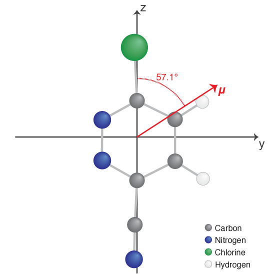
Figure 1: Sketch of the structure of the CPC molecule. The $x$-axis is perpendicular to the figure plane.

$i$	$B_{i}$ (MHz)	$\alpha_{ii}$ ($10^{-3}~{}\text{nm}^{3}$)	$\mu_{i}$ (D)
$x$	639.708	7.88	0
$y$	717.422	11.98	4.37
$z$	5905.0	22.24	2.83

Table 1: Rotational constants, polarizability components and components of the EDM of the CPC molecule Hansen et al. (2013). In the calculation of the rotational constants, the ³⁵Cl isotope was considered.

We use a field configuration equivalent to the experimental one Hansen et al. (2013), i. e., a Gaussian laser pulse with a peak intensity of $\textup{I}_{\textup{control}}=8.0\times 10^{11}~{}\text{W}/\text{cm}^{2}$ and a full-width at half maximum (FWHM) of 10 ns, and a tilted dc electric field with a field strength of 571 $\text{V}/\text{cm}$.

In the experiment Hansen et al. (2013), an inhomogeneous electric field was used to deflect the molecules according to the effective dipole moments of their rotational states Filsinger et al. (2009); Chang et al. (2015). The dispersed molecular beam then entered a velocity map imaging (VMI) spectrometer where it was crossed by the alignment and probe laser pulses. A state-selection of the sample was carried out by focusing the laser beams on the most deflected molecules, which are the ones in the lowest-energy rotational states Chang et al. (2015). The alignment and orientation of the CPC molecules was measured by Coulomb explosion imaging of ionic fragments onto a screen perpendicular to the dc electric field. The measured orientation corresponds to the average orientation of the molecules occupying different rotational states in the state-selected molecular ensemble.

The degree of orientation is experimentally quantified by the ratio $\text{N}_{\text{up}}/\text{N}_{\text{tot}}$ of Cl⁺ ions that are detected in the upper half of the screen to the total number of detected ions. In our calculations, we determine this orientation ratio by projecting the 3D probability density onto a 2D screen perpendicular to the dc electric field Omiste et al. (2011). Here, we take into account the probe selectivity for a probe pulse that is linearly polarized parallel to the screen. The volume effect due to the spatial intensity profiles of the alignment and probe lasers is not included in this work. We mimic the state-selection, which results in a non-thermal population distribution, by using a thermal ensemble at a temperature of 200 mK, which is lower than the (1 K) rotational temperature of the non-deflected molecular sample and was found to describe the non-thermal experimental ensemble well. We solve the TDSE for each state $\left|\psi_{\gamma}\right>$ in the thermal ensemble and determine the thermal orientation ratio as

$$\frac{\text{N}_{\text{up}}}{\text{N}_{\text{tot}}}=\sum_{\gamma}w^{T}_{\gamma}\frac{\text{N}_{\text{up}}^{\gamma}}{\text{N}_{\text{tot}}^{\gamma}}$$ (4)

with the thermal weights according to a Boltzmann distribution

$$w^{T}_{\gamma}=\frac{e^{-E_{\gamma}/k_{B}T}}{\sum_{\gamma}e^{-E_{\gamma}/k_{B}T}}$$ (5)

with the field-free energy $E_{\gamma}$ of the state $\left|\psi_{\gamma}\right>$. For the thermal ensemble at 200 mK, we take into account the 50 lowest lying rotational states of each irreducible representation, i. e., 100 rotational states are included in the sums (4) and (5).

III Orientation of a thermal ensemble and comparison to experimental results

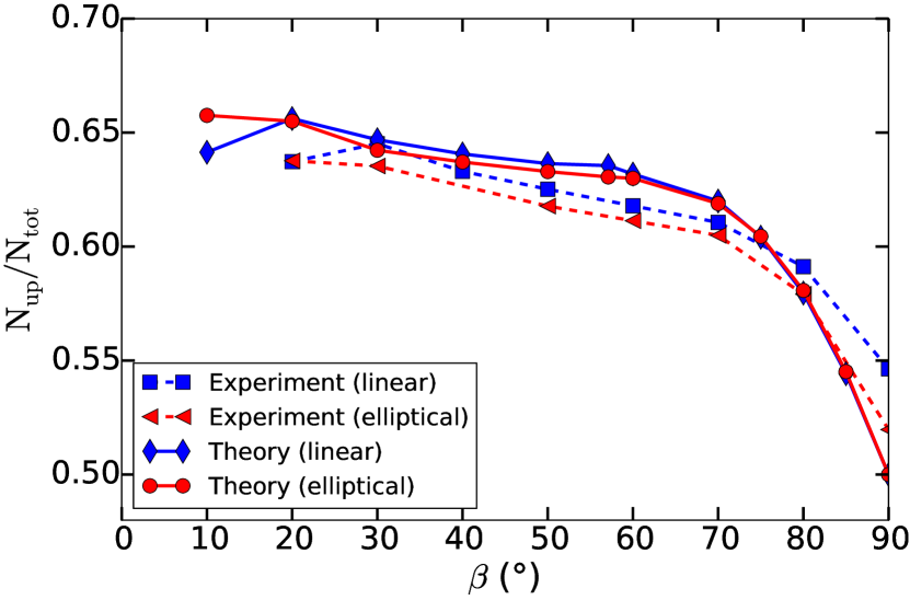
Figure 2: The orientation ratio $\text{N}_{\text{up}}/\text{N}_{\text{tot}}$ at the peak of the laser pulse, $\textup{I}_{\textup{control}}=8.0\times 10^{11}~{}\text{W}/\text{cm}^{2}$, as a function of $\beta$ for linearly and elliptically polarized pulses, computed for a thermal ensemble at $T=200$ mK (red diamonds and blue circles, respectively) and experimental results for a state-selected sample (red squares and blue triangles), see Fig. 5 from ref. Hansen et al., 2013. The dc field strength is 571 $\text{V}/\text{cm}$.

Fig. 2 shows the theoretical orientation for a thermal ensemble at $T=200$ mK at the control laser peak as a function of the angle $\beta$ between the dc field and the LFF $Z$-axis for linearly and elliptically polarized laser fields. These results are in very good agreement with the experimental orientation ratios for the state-selected molecular sample, which are reproduced from ref. Hansen et al., 2013. We observe similar results for the linearly and elliptically polarized laser fields: The orientation of the thermal ensemble increases smoothly as the static field is rotated towards the (major) polarization axis of the laser, and reaches values of $\text{N}_{\text{up}}/\text{N}_{\text{tot}}\sim 0.65$ for small $\beta$. For linear polarization, $\text{N}_{\text{up}}/\text{N}_{\text{tot}}$ decreases for $\beta=10\,^{\circ}$ due to the employed geometry of the experimental setup, which cannot correctly measure the orientation for parallel fields Nielsen et al. (2012). Overall, our time-dependent description of the mixed-field orientation of state-selected CPC reproduces the features of the experimentally observed behavior well. In particular, we find a good agreement between the experimental and theoretical orientation ratio for $\beta\lesssim 70\,^{\circ}$. For $\beta=90\,^{\circ}$, the experimental ensemble shows a small orientation which contradicts the theoretical prediction of no orientation for perpendicular fields. This could be due to experimental imperfections such as misalignment of the dc field, the polarization axis and detector screen or due to the influence of the probe laser. We point out that the smooth behavior of $\text{N}_{\text{up}}/\text{N}_{\text{tot}}$ is a consequence of the ensemble average. The orientation of an individual state might strongly depend on $\beta$ due to highly non-adiabatic effects appearing in the rotational dynamics, see section IV below. These non-adiabatic effects are masked by the ensemble average.

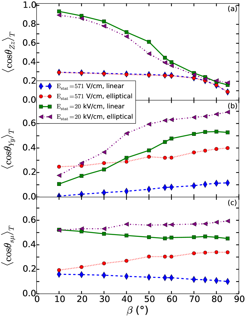
Figure 3: For a thermal ensemble at $T=200$ mK, the expectation values (a) $\langle\cos\theta_{Zz}\rangle_{T}$, (b) $\langle\cos\theta_{Yy}\rangle_{T}$ and (c) $\langle\cos\theta_{s\mu}\rangle_{T}$ at the laser peak intensity as a function of $\beta$ for a linearly polarized ac field and with $\textup{E}_{\textup{stat}}=571$ $\text{V}/\text{cm}$ (blue diamonds) and $\textup{E}_{\textup{stat}}=20$ $\text{kV}/\text{cm}$ (green squares) as well as for an elliptically polarized ac field with $\textup{E}_{\textup{stat}}=571$ $\text{V}/\text{cm}$ (red circles) and $\textup{E}_{\textup{stat}}=20$ $\text{kV}/\text{cm}$ (purple triangles).

Fig. 3 shows the calculated expectation values of the orientation cosines along the LFF $Z$ and $Y$-axes as well as the dc field direction for the same thermal sample and field configurations. The ratio $\text{N}_{\text{up}}/\text{N}_{\text{tot}}$ plotted in Fig. 2 quantifies the orientation of the MFF $z$-axis along the major polarization axis of the laser, providing information about 1D orientation, which is also characterized by $\langle\cos\theta_{Zz}\rangle_{T}$ shown in Fig. 3 (a). To investigate the 3D orientation, we additionally consider the expectation value $\langle\cos\theta_{Yy}\rangle_{T}$, shown in Fig. 3 (b), which measures the orientation of the MFF $y$-axis along the LFF $Y$-axis. The orientation of the EDM along the dc field direction is quantified by $\langle\cos\theta_{s\mu}\rangle_{T}$, presented in Fig. 3 (c).

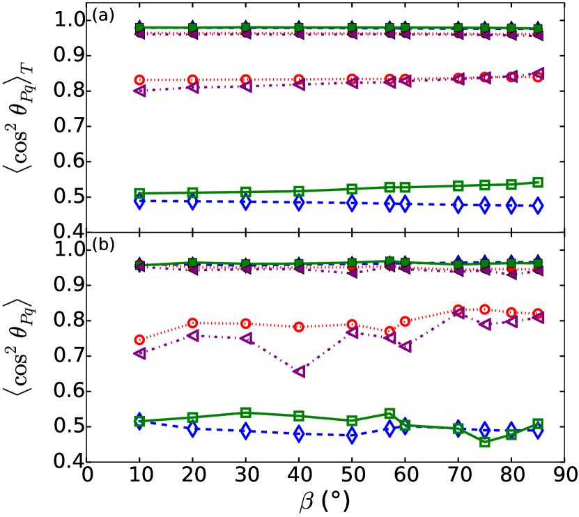
Figure 4: For (a) a thermal ensemble at $T=200$ mK, and (b) the state $|2_{12}1\rangle_{\text{t}}$, the expectation values $\langle\cos^{2}\theta_{Zz}\rangle$ (filled symbols) and $\langle\cos^{2}\theta_{Yy}\rangle$ (empty symbols) at the laser peak intensity as a function of $\beta$ for a linearly polarized ac field and with $\textup{E}_{\textup{stat}}=571$ $\text{V}/\text{cm}$ (blue diamonds) and $\textup{E}_{\textup{stat}}=20$ $\text{kV}/\text{cm}$ (green squares) as well as for an elliptically polarized ac field with $\textup{E}_{\textup{stat}}=571$ $\text{V}/\text{cm}$ (red circles) and $\textup{E}_{\textup{stat}}=20$ $\text{kV}/\text{cm}$ (purple triangles). The alignment along the LFF $Z$-axis is practically independent of all parameters with values of $\langle\cos^{2}\theta_{Zz}\rangle_{T}\approx 0.97$ and $\langle\cos^{2}\theta_{Zz}\rangle\approx 0.95$ for the thermal ensemble and the $|2_{12}1\rangle_{\text{t}}$ state, respectively.

For the linearly polarized laser field, the thermal sample is strongly aligned along the $Z$-axis, but not aligned along the $Y$-axis, as presented in Fig. 4. Strong 3D alignment is obtained with the elliptically polarized laser field, yielding $\langle\cos^{2}\theta_{Zz}\rangle_{T}\approx 0.95$ and $\langle\cos^{2}\theta_{Yy}\rangle_{T}\approx 0.83$ for all $\beta$. The alignment cosine $\langle\cos^{2}\theta_{Yy}\rangle_{T}$ shows a weak dependence on dc field and on the angle $\beta$.

The orientation of the thermal ensemble, Fig. 3 (a), shows a smooth behavior, with $\langle\cos\theta_{Zz}\rangle_{T}$ increasing from 0.09 to 0.29 for $\beta=85\,^{\circ}$ and $\beta=10\,^{\circ}$, respectively. This increase is not reproduced within the adiabatic picture, which predicts a $\beta$-independent orientation for a weak static electric field Hansen et al. (2013). The small orientation for $\beta$ close to $90\,^{\circ}$ in Fig. 3, obtained from the time-dependent results, can be explained by population transfer within pendular doublets formed as the laser intensity rises Nielsen et al. (2012); Omiste and González-Férez (2012, 2013); Trippel et al. (2015). At this field configuration, the oriented and antioriented adiabatic states within these near-degenerate pairs have similar contributions to the field-dressed dynamics reducing the orientation of the ensemble.

We now turn to the influence of a strong dc electric field on the orientation. For a dc field of 20 $\text{kV}/\text{cm}$, the thermal orientation $\langle\cos\theta_{Zz}\rangle_{T}$ rapidly increases as the angle between the fields decreases. For $\beta=10\,^{\circ}$, we find a strong orientation with $\langle\cos\theta_{Zz}\rangle_{T}=0.94$ and $\langle\cos\theta_{Zz}\rangle_{T}=0.90$ for linearly and elliptically polarized pulses, respectively. The enhancement of the orientation can be rationalized in terms of the rotational dynamics of each state in the thermal ensemble, i. e., the contributions of different instantaneous eigenstates of the Hamiltoninan (1) to the time-dependent wave function, see section IV. For low laser intensities, the interaction with the dc field is dominant, inducing a brute-force orientation of the EDM along the dc field direction. If $\beta$ is small, this brute-force orientation implies a moderate orientation of the MFF $z$-axis along the LFF $Z$-axis, due to the angle between the EDM and the MFF $z$-axis. As the laser intensity increases and becomes the dominant interaction, the strong dc field leads to preferred contributions of oriented pendular states to the time-dependent wave functions, which results in an enhancement of the orientation of the thermal ensemble.

Considering the orientation of the MFF $y$-axis along the LFF $Y$-axis, shown in Fig. 3 (b), the thermal ensemble is very weakly oriented for a linearly polarized pulse and $\textup{E}_{\textup{stat}}=571$ $\text{V}/\text{cm}$, reaching a maximum value of $\langle\cos\theta_{Yy}\rangle_{T}=0.12$ at $\beta=85\,^{\circ}$. However, a strong dc electric field induces a brute-force orientation of the EDM, and thus, a moderate orientation of the molecular $y$-axis, along the dc field direction before the laser pulse is turned on. This orientation of the MFF $y$-axis is maintained to some extend even in the presence of the laser field with $\langle\cos\theta_{Yy}\rangle_{T}$ increasing from 0.11 to 0.53 for $\beta=10\,^{\circ}$ and $\beta=85\,^{\circ}$, respectively, at the peak of the linearly-polarized laser pulse. Thus, a strong dc field combined with a linearly polarized ac field induces a significant 3D orientation for intermediate $\beta$. In contrast, even a weak dc field induces a moderate 3D orientation when combined with an elliptically polarized laser field. Here, the orientation along the $Y$-axis monotonically increases from $\langle\cos\theta_{Yy}\rangle_{T}=0.25$ to $\langle\cos\theta_{Yy}\rangle_{T}=0.40$ for $\beta=10\,^{\circ}$ to $\beta=85\,^{\circ}$, respectively. For $\textup{E}_{\textup{stat}}=20$ $\text{kV}/\text{cm}$, we find an enhancement of $\langle\cos\theta_{Yy}\rangle_{T}$, similar to the behavior of $\langle\cos\theta_{Zz}\rangle_{T}$ for strong dc fields, but for increasing $\beta$. If $\beta$ is small, the influence of the static field along the $Y$-axis is not strong enough to, in general, achieve preferred contributions of oriented pendular states to the rotational dynamics of excited states in the thermal ensemble. As a result, for $\beta=10\,^{\circ}$ we encounter a few low-lying excited states in the molecular ensemble that are not oriented or even strongly antioriented along the $Y$-axis at the peak intensity. Compared to the weak dc field, $\langle\cos\theta_{Yy}\rangle_{T}$ is reduced at this angle. This effect disappears if the temperature is increased and more excited states contribute to the thermal ensemble.

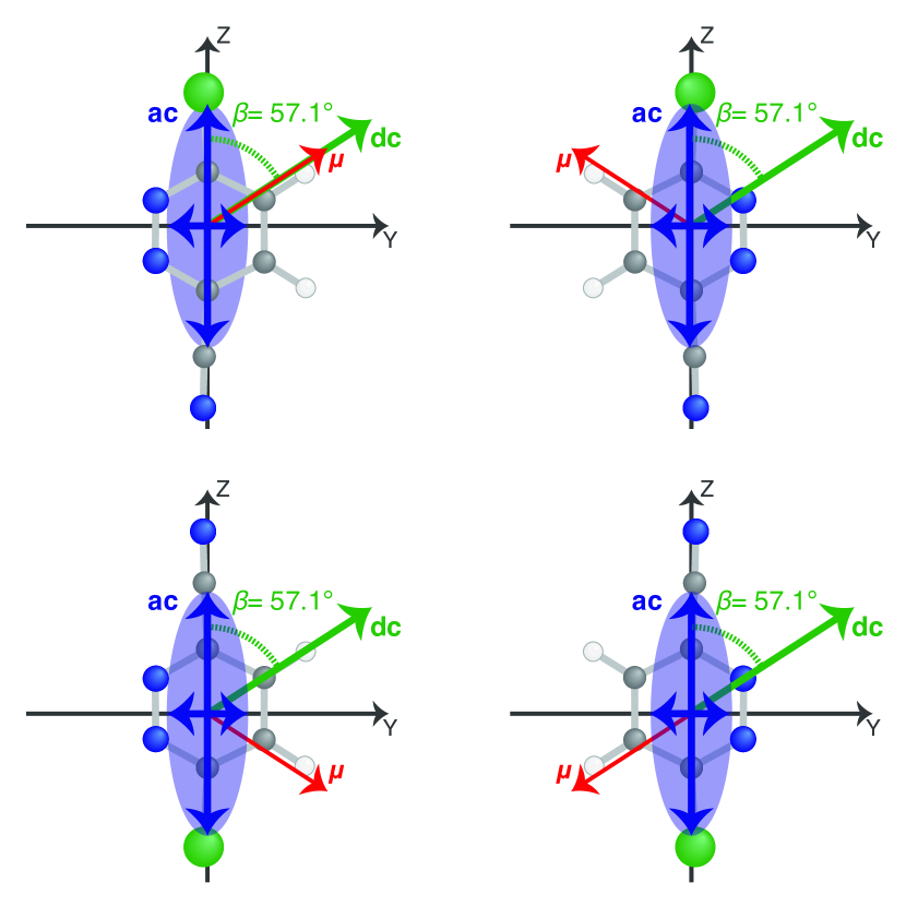
Figure 5: For an elliptically polarized laser field, the four possible orientations of the 3D aligned pendular states in the adiabatic picture.

Regarding the behavior of $\langle\cos\theta_{s\mu}\rangle_{T}$ in Fig. 3 (c), the orientation of the EDM along the dc field direction shows a weak dependence on $\beta$. For small angles between the ac and dc fields, $\langle\cos\theta_{s\mu}\rangle_{T}$ is approximately given by $\cos(57.1\,^{\circ})\langle\cos\theta_{Zz}\rangle_{T}$, since for these small angles it holds $\langle\cos\theta_{sz}\rangle_{T}\approx\langle\cos\theta_{Zz}\rangle_{T}$. Thus, for both polarizations we find similar values of $\langle\cos\theta_{s\mu}\rangle_{T}\approx 0.18$ and $\langle\cos\theta_{s\mu}\rangle_{T}\approx 0.5$ for the weak and strong dc fields, respectively. For $\beta=85\,^{\circ}$, the orientation of the EDM along the dc field direction is dominated by the behavior of $\langle\cos\theta_{Yy}\rangle_{T}$, and as a consequence, $\langle\cos\theta_{s\mu}\rangle_{T}$ is larger for the elliptically polarized laser field than for the linearly polarized laser field. The decreasing (increasing) behavior of $\langle\cos\theta_{s\mu}\rangle_{T}$ versus $\beta$ for linear (elliptical) polarization is due to the larger contribution of $\langle\cos\theta_{sy}\rangle_{T}$, since $\cos(57.1\,^{\circ})<\sin(57.1\,^{\circ})$. In addition, for the linear polarized case we find that $\langle\cos\theta_{Yy}\rangle_{T}$ for $\beta=85\,^{\circ}$ is smaller than $\langle\cos\theta_{Zz}\rangle_{T}$ for $\beta=10\,^{\circ}$ for both dc field strengths. For $\beta=57.1\,^{\circ}$, the angles between the ac and dc fields and between the EDM and the MPA coincide, and a maximum of $\langle\cos\theta_{s\mu}\rangle_{T}$ could be expected for the 3D aligned sample in an elliptically polarized laser field. However, this is not the case since the orientation of the EDM is obtained from the average over the four possible orientations of the adiabatic pendular states, shown in Fig. 5, which contribute to the time-dependent wave function of each state in the thermal ensemble.

To summarize, a significant 3D orientation is obtained for intermediate angles $\beta$, a strong dc field and both, linear and elliptical, laser polarizations. The degree of orientation of the MFF $y$-axis along the LFF $Y$-axis is larger for an elliptically polarized pulse than for a linearly polarized one, whereas the orientation of the MFF $z$-axis along the LFF $Z$-axis is similar in both cases. This implies that to achieve a large 3D orientation an elliptically polarized laser is recommended. Nevertheless, we point out that the naive picture of achieving 3D orientation by fixing one molecular axis, namely the MPA, with a linearly polarized laser field and a second axis, the EDM, with a dc electric field does (only) work in the limit of strong laser and strong dc electric fields.

IV Field-dressed dynamics

To analyze the dynamics of individual excited states for the different field configurations in detail, we choose the state $|2_{12}1\rangle_{\text{t}}$ as a prototypical example. Energetically, it is the 14th and 19th excited state of the representation with even parity under the reflection $\sigma_{YZ}$ for $\textup{E}_{\textup{stat}}=571$ $\text{V}/\text{cm}$ and $\textup{E}_{\textup{stat}}=20$ $\text{kV}/\text{cm}$, respectively. In Fig. 6 the orientation cosines $\langle\cos\theta_{Zz}\rangle$, $\langle\cos\theta_{Yy}\rangle$ and $\langle\cos\theta_{s\mu}\rangle$ at the peak intensity are presented as a function of $\beta$.

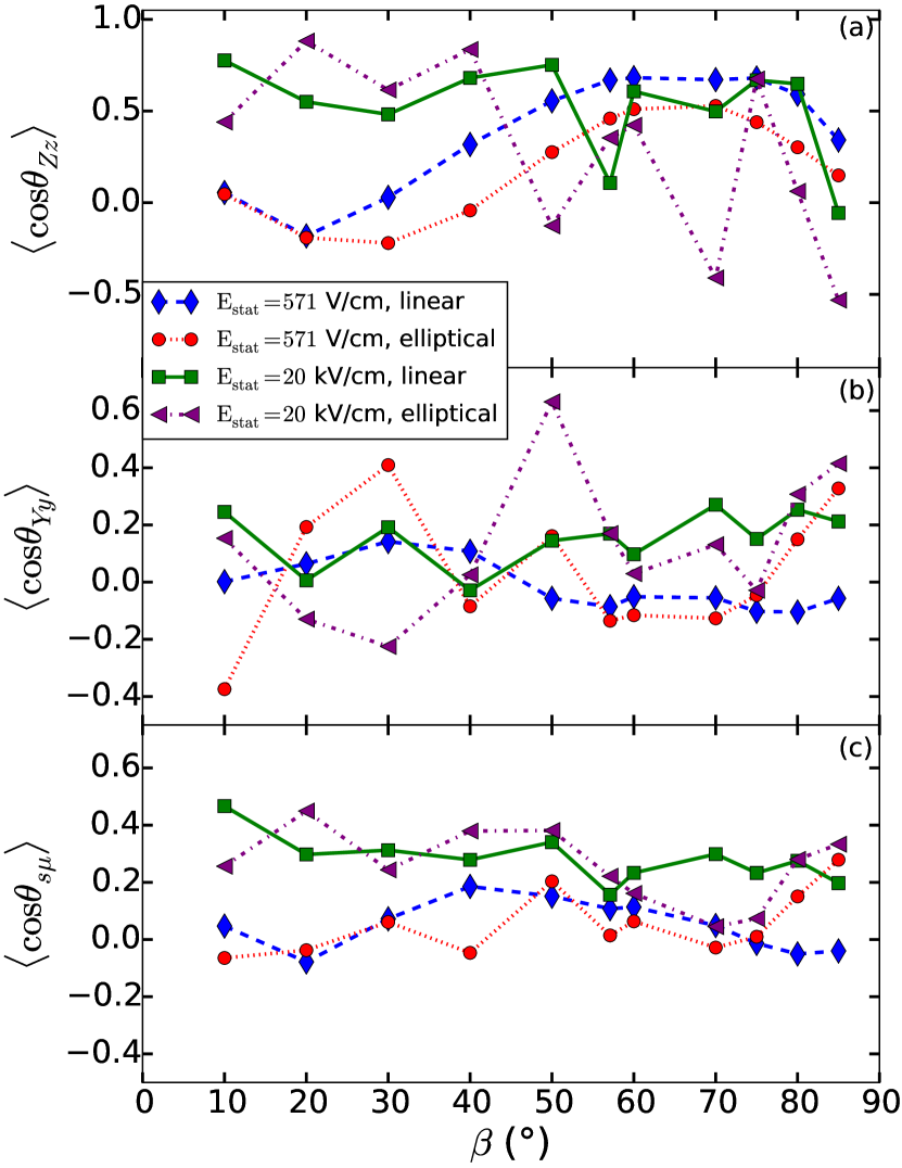
Figure 6: The expectation values (a) $\langle\cos\theta_{Zz}\rangle$, (b) $\langle\cos\theta_{Yy}\rangle$ and (c) $\langle\cos\theta_{s\mu}\rangle$ for the state $|2_{12}1\rangle_{\text{t}}$ at the peak intensity as a function of $\beta$ for a linearly polarized ac field and dc field strength $\textup{E}_{\textup{stat}}=571$ $\text{V}/\text{cm}$ (blue diamonds) and $\textup{E}_{\textup{stat}}=20$ $\text{kV}/\text{cm}$ (green squares) as well as for an elliptically polarized ac field and dc field strength $\textup{E}_{\textup{stat}}=571$ $\text{V}/\text{cm}$ (red circles) and $\textup{E}_{\textup{stat}}=20$ $\text{kV}/\text{cm}$ (purple triangles).

The smooth $\beta$-dependence found for the orientation of the thermal ensemble is not reflected in the final orientation of the state $|2_{12}1\rangle_{\text{t}}$. For instance, depending on the angle $\beta$, this state can be strongly 1D or 3D oriented, antioriented, or not oriented. However, certain features of the orientation of the thermal average can also be observed for the state $|2_{12}1\rangle_{\text{t}}$ as well as for most other states contributing to the ensemble average at 200 mK. In particular, the significant orientation along the $Z$-axis for a strong dc field and small $\beta$ and the decreasing orientation along the $Z$-axis for a weak dc field in the region $75\,^{\circ}\lesssim\beta<90\,^{\circ}$. However, the exact orientation for a specific field configuration can only be determined from time-dependent calculations. In contrast, the alignment along the the $Z$-axis of the state $|2_{12}1\rangle_{\text{t}}$, shown in Fig. 4 (b), does not depend on $\beta$ and resembles the alignment of the thermal sample. The alignment cosine $\langle\cos^{2}\theta_{Yy}\rangle$ shows a weak dependence on the angle between the ac and dc fields due to contributions of highly excited pendular states that are weakly aligned along the $Y$-axis.

The rotational dynamics shows highly non-adiabatic effects due to $M$-manifold splitting, avoided crossings and the formation of pendular doublets and quadruplets Omiste and González-Férez (2013, 2016). The importance of each of these effects depends strongly on the field configuration, i. e., the ac and dc field strengths, the angle $\beta$ between the fields, and the polarization and temporal profile of the laser pulse. In this section, we investigate the influence of these non-adiabatic phenomena on the mixed-field orientation. For illustration, the time evolution of the rotational dynamics of the $|2_{12}1\rangle_{\text{t}}$ state and the orientation cosines of the adiabatic pendular states are shown in movies provided in the supplementary material (see section VI).

IV.1 Linearly polarized laser

We start by analyzing the dynamics for a linearly polarized laser field. Even at low intensities, the dynamics is highly complicated. This is illustrated in Fig. 7 (a) and (b), which show the squares of the projection of the time-dependent wave function onto the adiabatic basis formed by the eigenstates of the instantaneous Hamiltonian (1). The dynamics is shown for a linearly polarized laser field through the intensity regime $10^{9}~{}\text{W}/\text{cm}^{2}\leq{}I(t)\leq 10^{10}$ $\text{W}/\text{cm}^{2}$ and both dc field strengths, $\textup{E}_{\textup{stat}}=571$ $\text{V}/\text{cm}$ and $\textup{E}_{\textup{stat}}=20$ $\text{kV}/\text{cm}$. For this example we chose $\beta=57.1\,^{\circ}$, which corresponds to the angle between EDM and MPA.

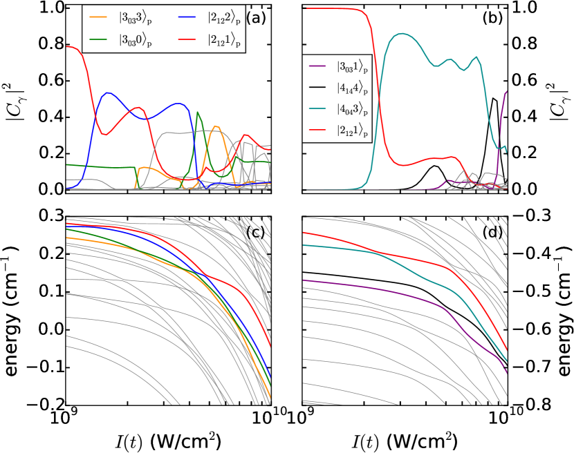
Figure 7: The squares of the projection of the time-dependent wave function onto the adiabatic-pendular-state basis of the state $|2_{12}1\rangle_{\text{t}}$, for a linearly polarized ac field through the field-strength regime $1.0\times 10^{9}$ $\text{W}/\text{cm}^{2}$ $\leq I(t)\leq$ $1.0\times 10^{10}$ $\text{W}/\text{cm}^{2}$ and dc field strengths of (a) $\textup{E}_{\textup{stat}}=571$ $\text{V}/\text{cm}$ and (b) $\textup{E}_{\textup{stat}}=20$ $\text{kV}/\text{cm}$. Energy level structure for the same intensities and dc field strengths (c) $\textup{E}_{\textup{stat}}=571$ $\text{V}/\text{cm}$ and (d) $\textup{E}_{\textup{stat}}=20$ $\text{kV}/\text{cm}$. The angle between the ac and dc fields is $\beta=57.1\,^{\circ}$.

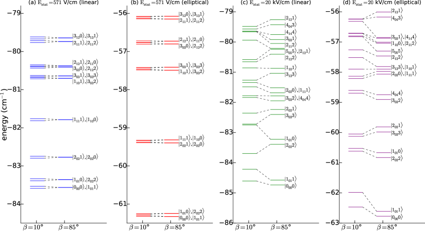
Figure 8: The energies of the 20 lowest lying adiabatic pendular states with even parity under reflection on the plane containing the ac and dc fields, at the peak intensity for (a) linearly polarized ac field and $\textup{E}_{\textup{stat}}=571$ $\text{V}/\text{cm}$, (b) elliptically polarized ac field and $\textup{E}_{\textup{stat}}=571$ $\text{V}/\text{cm}$, (c) linearly polarized ac field and $\textup{E}_{\textup{stat}}=20$ $\text{kV}/\text{cm}$, (d) elliptically polarized ac field and $\textup{E}_{\textup{stat}}=20$ $\text{kV}/\text{cm}$.

For a weak dc field of 571 $\text{V}/\text{cm}$, the population of the adiabatic pendular state $|2_{12}1\rangle_{\text{p}}$ is already significantly reduced at $1.0\times 10^{9}$ $\text{W}/\text{cm}^{2}$ compared to the laser field-free value of 1.0, see left side of Fig. 7 (a). This is due to population transfer at the splitting of the $|2_{12}M\rangle_{\text{p}}$ manifold with $M=1,2$ occurring at even lower intensities Omiste and González-Férez (2016). In contrast, for $\textup{E}_{\textup{stat}}=20$ $\text{kV}/\text{cm}$, the energy gap between the states within this manifold is so large that their coupling is significantly reduced, preventing population transfer within the manifold as the ac field is turned on.

In this low intensity regime, the large number of avoided crossings, see Fig. 7 (c) and (d), is the main source of the non-adiabatic behavior and leads to many adiabatic pendular states being involved in the dynamics. At each avoided crossing, the energy spacing among the involved pendular states strongly depends on the dc field strength and the angle between the ac and dc fields. Thus, the adiabatic pendular states contributing to the time-dependent wave function significantly vary for the dc field strengths considered here, c. f. Fig. 7 (a) and (b). By changing the angle $\beta$ or any other field parameter, the contributions of the adiabatic pendular states to the time-dependent wave function also vary strongly (not shown here). We emphasize that avoided crossings play an important role during the whole rotational dynamics of excited states and are one of the main sources of non-adiabatic effects. The dynamics through an avoided crossing depends, additionally, on the temporal profile of the laser. Achieving completely adiabatic dynamics at arbitrary avoided crossings, i. e., no population transfer between the involved pendular states, would be very challenging since it requires an extremely slowly increasing intensity due to the extremely narrow spacing between the involved states; i. e., to achieve adiabatic dynamics corresponding to the energy and field-strength range presented in Fig. 7 and Fig. 10 microsecond-long laser pulses or a continuous-wave control laser Deppe et al. (2015) would be necessary.

At stronger laser fields, quasi-degenerate pendular doublets are formed providing an additional source of non-adiabatic effects. During the doublet formation with increasing $I(t)$, the energy splitting and the directional properties of the two pendular states change in a way that depends strongly on the external field parameters, in particular the dc field strength and the angle $\beta$. Thus, the influence of the doublet formation on the rotational dynamics and the mixed-field orientation at the peak intensity varies significantly if the field configuration is modified.

For $\textup{E}_{\textup{stat}}=571$ $\text{V}/\text{cm}$, the pendular doublets can be clearly observed for all values of $\beta$, see Fig. 8 (a), which shows the energies of the 20 lowest lying adiabatic pendular states at the peak of the laser pulse for $\beta=10\,^{\circ}$ and $\beta=85\,^{\circ}$. The energy separation within these pendular doublets, $\Delta{E}\sim 2\textup{E}_{\textup{stat}}\mu_{z}\cos\beta$, decreases as the dc field is rotated towards the perpendicular field configuration. For $\beta=85\,^{\circ}$, the small energy splitting and rapid formation of the pendular doublets with increasing laser intensity leads to a redistribution of the population within the quasi-degenerate doublets. This redistribution of the population for $\beta=85\,^{\circ}$ can be observed in the projection of the wave function onto the adiabatic basis at the peak intensity, shown in Fig. 9 (a), where the two adiabatic pendular states in several doublets have similar weights. This can also be observed in the field-dressed-dynamics movies in the supplementary material (see section VI). Since the quasi-degenerate doublets consist of strongly aligned pendular states that are oriented in opposite directions along the LFF $Z$-axis, the overall orientation of the state $|2_{12}1\rangle_{\text{t}}$ at the peak intensity decreases as $\beta$ approaches $90\,^{\circ}$, see Fig. 6 (a). A similar population redistribution within the pendular doublets also occurs for other excited states, and, as a result, the orientation of the thermal ensemble in Fig. 3 (a) decreases as $\beta$ approaches $90\,^{\circ}$.

Figure 9: For the state $|2_{12}1\rangle_{\text{t}}$, the squares of the projection of the wave function at the peak of a linearly polarized laser pulse onto the adiabatic pendular states as a function of $\beta$ and the index of the pendular states according to energetic order. The dc field strength is (a) $\textup{E}_{\textup{stat}}=571$ $\text{V}/\text{cm}$ and (b) $\textup{E}_{\textup{stat}}=20$ $\text{kV}/\text{cm}$. The index of the adiabatic pendular state $|2_{12}1\rangle_{\text{p}}$ is 14 and 19 for the weak and strong dc field, respectively.

As $\beta$ decreases, the increasing $Z$-component of the dc field leads to larger energy splitting between the two adiabatic pendular states in the doublets. As a result, for small $\beta$ we find less population transfer among the involved adiabatic pendular states than for $\beta$ close to $90\,^{\circ}$. The weights of two adiabatic pendular states forming a quasi-degenerate pair can differ strongly at the peak intensity for $\beta\lesssim 70\,^{\circ}$, c. f. Fig. 9 (a). In the final population distribution in Fig. 9 (a), we encounter gaps of unpopulated pendular states that can be explained by population transfer at avoided crossings occurring at high intensities. When the pendular doublets are already formed, we encounter avoided crossings involving four adiabatic pendular states. In these highly non-adiabatic avoided crossings, the population of the oriented (antioriented) state passes to the oriented (antioriented) state of the adjacent doublet (see section VI). Due to this mainly diabatic rotational dynamics at high intensities only a few adiabatic pendular states, distributed over a wide range of energies, significantly contribute to the final wave function. These pendular states mainly determine the orientation at different $\beta$. Depending on the angle between the ac and dc fields, the contributions of either oriented or antioriented adiabatic states are dominant in the final wave function. This leads to the oscillating behavior of $\langle\cos\theta_{Zz}\rangle$ versus $\beta$ in Fig. 6 (a).

For a strong dc field of $\textup{E}_{\textup{stat}}=20$ $\text{kV}/\text{cm}$, the arrangement in pendular doublets can still be observed for $\beta$ close to $90\,^{\circ}$, where the energy separation within the doublets is much larger than for a weak dc field, see Fig. 8 (c). For small angles, the lower lying adiabatic states do not form pendular doublets having opposite orientation, but there are nearly degenerate adiabatic states oriented in the same direction. For $\beta=85\,^{\circ}$, due to the large energy separation, the pendular doublet formation does not lead to a significant population transfer between the two pendular states as for a weak dc field and the same angle. Thus, the field-dressed dynamics for $\textup{E}_{\textup{stat}}=20$ $\text{kV}/\text{cm}$ is dominated by avoided crossings between neighboring levels. The population transfer occurring at these avoided crossings gives rise to a broad and homogeneous distribution of populated pendular states at the peak intensity, see Fig. 9 (b). As a result, we find similar contributions of oriented and antioriented adiabatic pendular states for $\beta=85\,^{\circ}$, giving rise to a small orientation along the $Z$-axis of the state $|2_{12}1\rangle_{\text{t}}$. We find other time-dependent excited states that are strongly oriented or antioriented at the peak intensity, depending on the weights of the adiabatic states in their final wave functions. The opposite orientations of these time-dependent states cancel in the thermal ensemble, which shows a weak orientation for $\beta=85\,^{\circ}$.

If $\beta$ is small, the initial brute-force orientation of the EDM, induced by the strong dc field, implies a significant orientation of the MFF $z$-axis along the LFF $Z$-axis before the laser pulse is turned on. For laser intensities above $1.0\times 10^{10}$ $\text{W}/\text{cm}^{2}$, the interaction with the ac field becomes dominant over the interaction with the dc field and the MPA becomes aligned along the $Z$-axis. Due to this strong confinement of the MPA, the orientation of many adiabatic pendular states along the $Z$-axis increases while some pendular states gradually become strongly antioriented. The change in the $\langle\cos\theta_{Zz}\rangle$ versus the laser intensity can be observed in the movies provided in the supplementary material (see section VI). The pendular states initially becoming antioriented in this intermediate intensity regime are mostly highly excited states that are not populated so that mainly oriented adiabatic states continue to contribute to the rotational dynamics in this regime. As the laser intensity increases further, we encounter numerous avoided crossings between these strongly oriented and strongly antioriented pendular states. At such an avoided crossing, the involved adiabatic pendular states interchange their directional properties, i. e., the previously oriented (antioriented) state becomes antioriented (oriented). Since these avoided crossings are traversed diabatically, the time-dependent wave function does not acquire population on the antioriented adiabatic pendular states. As a result, the distribution in Fig. 9 (b) shows gaps of unpopulated adiabatic states that are mainly antioriented at the peak intensity. Thus, at the peak intensity, the state $|2_{12}1\rangle_{\text{t}}$ is strongly oriented along the LFF $Z$-axis for small values of $\beta$, see Fig. 6 (a). The dynamics of other excited states shows a similar behavior, thus enhancing the orientation of the thermal ensemble as seen in Fig. 3 (a).

For $\beta$ close to $90\,^{\circ}$, i. e., small angles between the dc field and the LFF $Y$-axis, the initial brute-force orientation of the EDM implies an orientation of the MFF $y$-axis along the LFF $Y$-axis before the laser pulse is turned on. This orientation is maintained for several adiabatic pendular states even at the peak intensity but we also find other pendular states being weakly antioriented or not oriented (see section VI). This leads to an overall moderate orientation of the MFF $y$-axis along the LFF $Y$-axis for the state $|2_{12}1\rangle_{\text{t}}$ as well as the thermal average, for $\beta$ close to $90\,^{\circ}$, see Fig. 6 (b) and Fig. 3 (b). If $\beta$ is small, the dc electric field does not induce an initial orientation of the MFF $y$-axis along the LFF $Y$-axis. In the presence of the laser field, different time-dependent excited states may become moderately oriented in opposite directions or show no orientation along the LFF $Y$-axis at the peak intensity. Thus, the thermal ensemble shows a very small orientation $\langle\cos\theta_{Yy}\rangle_{T}$ for small $\beta$.

IV.2 Elliptically polarized laser

We now consider the rotational dynamics in elliptically polarized laser fields. In the absence of the dc field, the elliptically polarized ac field induces 3D alignment of the CPC molecules, with the $z$ and $y$ molecular axes aligned along the LFF $Z$ and $Y$-axes, respectively. Compared to the linearly polarized cases analyzed in the previous section, and since the total intensities for both polarizations are equal, the effective intensities of the elliptically polarized laser field along these two axes are weaker. This implies a smaller alignment along the $Y$-axis, as is illustrated in Fig. 4. In this section, we analyze how this change in the ac field polarization affects the rotational dynamics and mixed-field orientation.

For low intensities, $10^{9}~{}\text{W}/\text{cm}^{2}\leq{}I(t)\leq~{}10^{10}$ $\text{W}/\text{cm}^{2}$, the squares of the projection of the time-dependent wave function for the state $|2_{12}1\rangle_{\text{t}}$ are shown in Fig. 10 (a) and (b) for $\beta=57.1\,^{\circ}$ and $\textup{E}_{\textup{stat}}=571$ $\text{V}/\text{cm}$ and $\textup{E}_{\textup{stat}}=20$ $\text{kV}/\text{cm}$, respectively. In this intensity regime, we find a similarly complex dynamics as for a linearly polarized laser field presented in Fig. 7. For $\textup{E}_{\textup{stat}}=571$ $\text{V}/\text{cm}$ the splitting of the $|2_{12}M\rangle_{\text{p}}$ manifold at weaker intensities leads to population transfer among the two pendular states within this manifold. For a strong dc field with $\textup{E}_{\textup{stat}}=20$ $\text{kV}/\text{cm}$, this effect is not significant and the population of the state $|2_{12}1\rangle_{\text{p}}$, is still approximately 1.0 at $1.0\times 10^{9}$ $\text{W}/\text{cm}^{2}$. The large number of avoided crossings in Fig. 10 (c) and (d) dominate the rotational dynamics, which involves several adiabatic pendular states even for low intensities. Differences between the dynamics for linearly and elliptically polarized ac fields gain importance at higher intensities where the elliptically polarized ac field significantly influences the energy level structure and the directional features of the adiabatic pendular states.

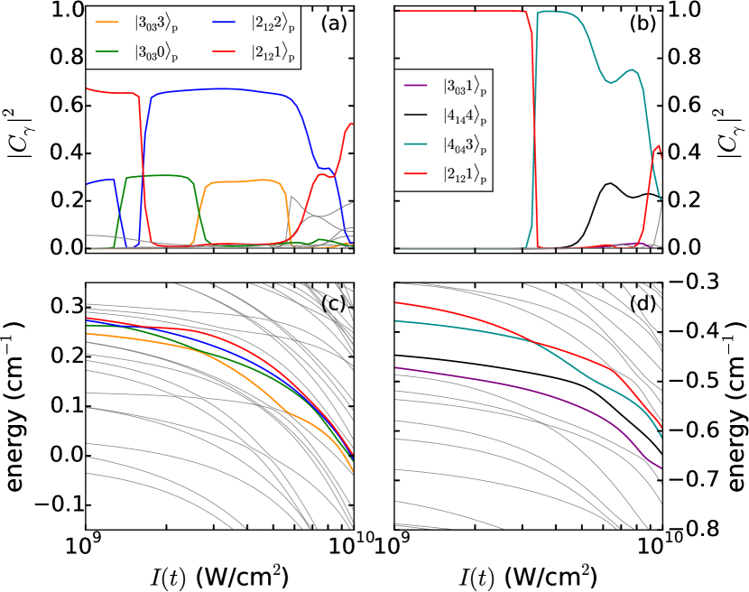
Figure 10: The squares of the projection of the time-dependent wave function onto the adiabatic-pendular-state basis of the state $|2_{12}1\rangle_{\text{t}}$, for an elliptically polarized ac field through the field-strength regime $1.0\times 10^{9}$ $\text{W}/\text{cm}^{2}$ $\leq I(t)\leq$ $1.0\times 10^{10}$ $\text{W}/\text{cm}^{2}$ and dc field strengths of (a) $\textup{E}_{\textup{stat}}=571$ $\text{V}/\text{cm}$ and (b) $\textup{E}_{\textup{stat}}=20$ $\text{kV}/\text{cm}$. Energy level structure for the same intensities and dc field strengths (c) $\textup{E}_{\textup{stat}}=571$ $\text{V}/\text{cm}$ and (d) $\textup{E}_{\textup{stat}}=20$ $\text{kV}/\text{cm}$. The angle between the ac and dc fields is $\beta=57.1\,^{\circ}$.

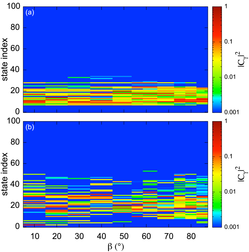
Figure 11: For the state $|2_{12}1\rangle_{\text{t}}$, the squares of the projection of the wave function at the peak of a elliptically polarized laser pulse onto the adiabatic pendular states as a function of $\beta$ and the index of the pendular states according to energetic order. The dc field strength is (a) $\textup{E}_{\textup{stat}}=571$ $\text{V}/\text{cm}$ and (b) $\textup{E}_{\textup{stat}}=20$ $\text{kV}/\text{cm}$. The index of the adiabatic pendular state $|2_{12}1\rangle_{\text{p}}$ is 14 and 19 for the weak and strong dc field, respectively.

Analogously to the linearly polarized ac field, near-degenerate pendular doublets are formed as the laser intensity increases. For $\textup{E}_{\textup{stat}}=571$ $\text{V}/\text{cm}$ and $I(t)\gtrsim 10^{11}$ $\text{W}/\text{cm}^{2}$, we additionally encounter the formation of near-degenerate quadruplets, after the doublets are already formed. This arrangement in doublets and quadruplets can be observed in the energies of the adiabatic pendular states at the peak intensity, shown in Fig. 8 (b). The energy separations between consecutive quadruplets are larger than between consecutive doublets in the case of a linearly polarized ac field. Due to the quadruplet formation for the elliptically polarized laser field, we find a smaller number of avoided crossings between near-degenerate groups of pendular states than for linear polarization. These features of the energy level structure limit the population transfer to highly excited states and the population at the peak intensity is confined to a small region of relatively low-lying adiabatic pendular states for all values of $\beta$, c. f. Fig. 11 (a) and section VI.

For the weak dc field and $\beta$ close to $90\,^{\circ}$, a redistribution of the population occurs during the formation of the near-degenerate doublets similar to the case of a linearly polarized ac field (see section VI). This is reflected in the weights of the adiabatic pendular states contributing to the time-dependent wave function at the peak intensity, c. f. Fig. 11 (a), where there are several neighboring adiabatic levels with similar contributions. This redistribution leads to the decrease of $\langle\cos\theta_{Zz}\rangle$ for $\beta\gtrsim 75\,^{\circ}$ for the state $|2_{12}1\rangle_{\text{t}}$ in Fig. 6 (a) and the thermal ensemble in Fig. 3 (a), similar to the case of a linearly polarized laser pulse. For $\beta=85\,^{\circ}$, the states forming each of the two doublets in a near-degenerate quadruplet are oriented in opposite directions along the LFF $Z$-axis, but in the same direction along the $Y$-axis (see section VI). Thus, the state $|2_{12}1\rangle_{\text{t}}$ shows a moderate orientation along the $Y$-axis at this angle see Fig. 6 (b). We find other time-dependent excited states that are antioriented at the peak intensity due to different adiabatic pendular states contributing to their rotational dynamics. In the thermal ensemble, the contributions of states, which are oriented along the $Y$-axis, become more dominant as $\beta$ approaches $90\,^{\circ}$, giving rise to the increase of $\langle\cos\theta_{Yy}\rangle$ for increasing $\beta$ in Fig. 3 (b).

For a strong dc electric field, pendular doublets can be observed for $\beta$ close to $90\,^{\circ}$ and some low-lying pendular states for small $\beta$. Near-degenerate quadruplets are not formed, see Fig. 8 (d). Thus, avoided crossings are the main source of non-adiabatic phenomena in the rotational dynamics at higher intensities.

For $\beta=10\,^{\circ}$, a qualitatively similar rotational dynamics can be observed for both, linear and elliptical, polarizations of the ac field, but with different adiabatic states contributing to the time-dependent wave functions (see section VI). The distributions of the population of adiabatic pendular states in the wave function at the peak intensity show the same features, i. e., the approximate number and range of contributing pendular states, in both cases, see Fig. 11 (b) and Fig. 9 (b). The state $|2_{12}1\rangle_{\text{t}}$ also shows a significant orientation of the MFF $z$-axis along the LFF $Z$-axis at the peak intensity of the elliptically polarized ac field, see Fig. 6 (a). However, since the weights of the adiabatic pendular states vary when the ac field polarization is changed, $\langle\cos\theta_{Zz}\rangle$ at $\beta=10\,^{\circ}$ differs for the linearly and elliptically polarized laser pulses.

Regarding the orientation along the LFF $Y$-axis for the strong dc field and the elliptically polarized ac field, the state $|2_{12}1\rangle_{\text{t}}$ shows an analogous behavior for $\beta=85\,^{\circ}$ as for the orientation along the LFF $Z$-axis for $\beta=10\,^{\circ}$. Once the ac field component along the LFF $Y$-axis is sufficiently strong to align the MFF $y$-axis along the LFF $Y$-axis, the initially brute-force-oriented adiabatic pendular states become either strongly oriented or strongly antioriented along this axis (see section VI). As this occurs, several pendular states becoming antioriented along the $Y$-axis have significant weights in the time-dependent wave function. As a result, the state $|2_{12}1\rangle_{\text{t}}$ only shows a moderate orientation of the MFF $y$-axis along the LFF $Y$-axis at the peak intensity, c. f. Fig. 6 (b). Other excited states may even be weakly antioriented. Thus, for the thermal ensemble, $\langle\cos\theta_{Yy}\rangle_{T}$ in Fig. 3 (b) is only moderately enhanced by the strong dc field.

To summarize, even if the field-dressed dynamics is highly non-adiabatic, the directional features of individual excited rotational states and, consequently, of the ensemble average, can be controlled to some extend. A significant orientation of the MFF $z$-axis along the LFF $Z$-axis can be achieved by applying a strong dc field for small values of $\beta$ and both a linearly and elliptically polarized laser field. An analogous enhancement of the orientation of the MFF $y$-axis along the LFF $Y$-axis is obtained for an elliptically polarized ac field and $\beta$ close to $90\,^{\circ}$.

V Conclusion

We present a time-dependent analysis of the rotational dynamics of a non-symmetric molecule in combined ac and dc electric fields. We investigate the influence of the dc field strength and the angle between the ac and dc fields during the turn-on of linearly and elliptically polarized laser pulses. Our theoretical study is focused on the prototypical CPC molecule, which has a permanent dipole moment with a direction that is neither parallel to any principle axis of inertia nor to any principle axis of polarizability.

Our computational results for a thermal ensemble at 200 mK agree quantitatively with mixed-field-orientation experiments of state-selected CPC molecules Hansen et al. (2013), including the 1D orientation along the $Z$-axis, and the smooth $\beta$-dependence of the orientation that could not be explained by the previous adiabatic description. Our time-dependent description also shows that in the experiment 3D orientation was achieved for the employed combination of the elliptically polarized laser pulse and the weak dc field.

The analysis of the time-dependent dynamics of individual states, which we described for the prototypical state $|2_{12}1\rangle_{\text{t}}$, shows highly non-adiabatic dynamics. These non-adiabaticities arise due to avoided crossings, $M$-manifold splitting, and the formation of pendular doublets and quadruplets. The relevance of these phenomena and the exact dynamics are highly dependent on the field parameters, e. g., the laser pulse, the dc field strength, and the angle between the two fields. Generally, the distribution of population over many adiabatic pendular states leads to a weak net orientation, because a priori as many oriented as antioriented pendular states are involved in the field-dressed dynamics. However, for strong dc electric fields, preferred contributions of oriented pendular states to the wave function are obtained and strong degrees of orientation are achieved even for rotationally excited states.

For a ground-state ensemble, which for complex molecules can be produced by state-specific guiding Putzke et al. (2011), adiabatic 3D orientation can be achieved by combining a long laser pulse with a moderately strong dc electric field. For excited states, although the dynamics is non-adiabatic, their directional features can be controlled to some degree by applying strong dc fields. Furthermore, we show that 3D orientation of a thermal ensemble can be achieved in two ways: Firstly, by combining a linearly polarized laser field with a strong dc electric field, effectively locking the MPA to the laser polarization axis and the EDM to the dc electric field direction. Secondly, by combining an elliptically polarized laser field with a strong dc electric field to induce mixed-field orientation of the 3D aligned sample.

While the current work is focused on the prototypical complex molecule CPC, similar rotational dynamics are expected for other non-symmetric molecules. Even if the principle axes of inertia and polarizability are non-parallel, mixed-field orientation is expected. Since the non-adiabatic effects strongly depend on the molecular properties, accurate predictions of the results of mixed-field experiments requires an accurate description, e.g., a TDSE analysis of the rotational dynamics. The present work paves the way to an accurate description of the mixed-field orientation of large molecules in general, which is highly relevant for molecular-frame imaging experiments of complex molecules, where experimental determinations of the degree of alignment and orientation become very difficult and corresponding simulations of the angular control are necessary to analyze the experimental data Filsinger et al. (2011); Barty, Küpper, and Chapman (2013).

VI Supplementary Material

See supplementary material for movies of the field-dressed rotational dynamics of the state $|2_{12}1\rangle_{\text{t}}$ and the orientation cosines of the adiabatic pendular states.

VII Acknowledgements

We gratefully acknowledge Juan J. Omiste for developing the computer code to solve the time-dependent Schrödinger equation.

In addition to DESY, this work has been supported by the Helmholtz Association “Initiative and Networking Fund”, by the Deutsche Forschungsgemeinschaft (DFG) through the excellence cluster “The Hamburg Center for Ultrafast Imaging – Structure, Dynamics and Control of Matter at the Atomic Scale” (CUI, EXC1074), and by the European Research Council through the Consolidator Grant COMOTION (ERC-Küpper-614507). R.G.F. gratefully acknowledges financial support by the Spanish project FIS2014-54497-P (MINECO) and by the Andalusian research group FQM-207 and the grant P11-FQM-7276.

References

- Spence and Doak (2004) J. C. H. Spence and R. B. Doak, “Single molecule diffraction,” Phys. Rev. Lett. 92, 198102 (2004).
- Barty, Küpper, and Chapman (2013) A. Barty, J. Küpper, and H. N. Chapman, “Molecular imaging using x-ray free-electron lasers,” Annu. Rev. Phys. Chem. 64, 415–435 (2013).
- Miller (2014) R. J. D. Miller, “Mapping atomic motions with ultrabright electrons: The chemists’ gedanken experiment enters the lab frame,” Annu. Rev. Phys. Chem. 65, 583–604 (2014).
- Brooks (1976) P. R. Brooks, “Reactions of oriented molecules,” Science 193, 11 (1976).
- Rakitzis, van den Brom, and Janssen (2004) T. P. Rakitzis, A. J. van den Brom, and M. H. M. Janssen, “Directional dynamics in the photodissociation of oriented molecules,” Science 303, 1852–1854 (2004).
- Meckel et al. (2008) M. Meckel, D. Comtois, D. Zeidler, A. Staudte, D. Pavičić, H. C. Bandulet, H. Pépin, J. C. Kieffer, R. Dörner, D. M. Villeneuve, and P. B. Corkum, “Laser-induced electron tunneling and diffraction,” Science 320, 1478–1482 (2008).
- Bisgaard et al. (2009) C. Z. Bisgaard, O. J. Clarkin, G. Wu, A. M. D. Lee, O. Geßner, C. C. Hayden, and A. Stolow, “Time-resolved molecular frame dynamics of fixed-in-space CS2 molecules,” Science 323, 1464–1468 (2009).
- Holmegaard et al. (2010) L. Holmegaard, J. L. Hansen, L. Kalhøj, S. L. Kragh, H. Stapelfeldt, F. Filsinger, J. Küpper, G. Meijer, D. Dimitrovski, M. Abu-samha, C. P. J. Martiny, and L. B. Madsen, “Photoelectron angular distributions from strong-field ionization of oriented molecules,” Nat. Phys. 6, 428 (2010), arXiv:1003.4634 [physics] .
- Itatani et al. (2004) J. Itatani, J. Levesque, D. Zeidler, H. Niikura, H. Pépin, J. C. Kieffer, P. B. Corkum, and D. M. Villeneuve, “Tomographic imaging of molecular orbitals,” Nature 432, 867–871 (2004).
- Vozzi et al. (2011) C. Vozzi, M. Negro, F. Calegari, G. Sansone, M. Nisoli, S. De Silvestri, and S. Stagira, “Generalized molecular orbital tomography,” Nat. Phys. 7, 822–826 (2011).
- Kraus, Baykusheva, and Wörner (2014) P. M. Kraus, D. Baykusheva, and H. J. Wörner, “Two-pulse field-free orientation reveals anisotropy of molecular shape resonance,” Phys. Rev. Lett. 113, 023001 (2014), arXiv:1311.3923 [physics.chem-ph] .
- Hensley, Yang, and Centurion (2012) C. J. Hensley, J. Yang, and M. Centurion, “Imaging of isolated molecules with ultrafast electron pulses,” Phys. Rev. Lett. 109, 133202 (2012).
- Küpper et al. (2014) J. Küpper, S. Stern, L. Holmegaard, F. Filsinger, A. Rouzée, A. Rudenko, P. Johnsson, A. V. Martin, M. Adolph, A. Aquila, S. Bajt, A. Barty, C. Bostedt, J. Bozek, C. Caleman, R. Coffee, N. Coppola, T. Delmas, S. Epp, B. Erk, L. Foucar, T. Gorkhover, L. Gumprecht, A. Hartmann, R. Hartmann, G. Hauser, P. Holl, A. Hömke, N. Kimmel, F. Krasniqi, K.-U. Kühnel, J. Maurer, M. Messerschmidt, R. Moshammer, C. Reich, B. Rudek, R. Santra, I. Schlichting, C. Schmidt, S. Schorb, J. Schulz, H. Soltau, J. C. H. Spence, D. Starodub, L. Strüder, J. Thøgersen, M. J. J. Vrakking, G. Weidenspointner, T. A. White, C. Wunderer, G. Meijer, J. Ullrich, H. Stapelfeldt, D. Rolles, and H. N. Chapman, “X-ray diffraction from isolated and strongly aligned gas-phase molecules with a free-electron laser,” Phys. Rev. Lett. 112, 083002 (2014), arXiv:1307.4577 [physics] .
- Yang et al. (2016) J. Yang, M. Guehr, T. Vecchione, M. S. Robinson, R. Li, N. Hartmann, X. Shen, R. Coffee, J. Corbett, A. Fry, K. Gaffney, T. Gorkhover, C. Hast, K. Jobe, I. Makasyuk, A. Reid, J. Robinson, S. Vetter, F. Wang, S. Weathersby, C. Yoneda, M. Centurion, and X. Wang, “Diffractive imaging of a rotational wavepacket in nitrogen molecules with femtosecond megaelectronvolt electron pulses,” Nat. Commun. 7, 11232 (2016).
- Loesch and Remscheid (1990) H. J. Loesch and A. Remscheid, “Brute force in molecular reaction dynamics: A novel technique for measuring steric effects,” J. Chem. Phys. 93, 4779 (1990).
- Friedrich and Herschbach (1999) B. Friedrich and D. Herschbach, “Enhanced orientation of polar molecules by combined electrostatic and nonresonant induced dipole forces,” J. Chem. Phys. 111, 6157 (1999).
- Stapelfeldt and Seideman (2003) H. Stapelfeldt and T. Seideman, “Colloquium: Aligning molecules with strong laser pulses,” Rev. Mod. Phys. 75, 543–557 (2003).
- Holmegaard et al. (2009) L. Holmegaard, J. H. Nielsen, I. Nevo, H. Stapelfeldt, F. Filsinger, J. Küpper, and G. Meijer, “Laser-induced alignment and orientation of quantum-state-selected large molecules,” Phys. Rev. Lett. 102, 023001 (2009), arXiv:0810.2307 [physics.chem-ph] .
- Ghafur et al. (2009) O. Ghafur, A. Rouzee, A. Gijsbertsen, W. K. Siu, S. Stolte, and M. J. J. Vrakking, “Impulsive orientation and alignment of quantum-state-selected NO molecules,” Nat. Phys. 5, 289–293 (2009).
- Nielsen et al. (2012) J. H. Nielsen, H. Stapelfeldt, J. Küpper, B. Friedrich, J. J. Omiste, and R. González-Férez, “Making the best of mixed-field orientation of polar molecules: A recipe for achieving adiabatic dynamics in an electrostatic field combined with laser pulses,” Phys. Rev. Lett. 108, 193001 (2012), arXiv:1204.2685 [physics.chem-ph] .
- Trippel et al. (2015) S. Trippel, T. Mullins, N. L. M. Müller, J. S. Kienitz, R. González-Férez, and J. Küpper, “Two-state wave packet for strong field-free molecular orientation,” Phys. Rev. Lett. 114, 103003 (2015), arXiv:1409.2836 [physics] .
- Hansen et al. (2013) J. L. Hansen, J. J. Omiste, J. H. Nielsen, D. Pentlehner, J. Küpper, R. González-Férez, and H. Stapelfeldt, “Mixed-field orientation of molecules without rotational symmetry,” J. Chem. Phys. 139, 234313 (2013), arXiv:1308.1216 [physics] .
- Omiste et al. (2011) J. J. Omiste, M. Gaerttner, P. Schmelcher, R. González-Férez, L. Holmegaard, J. H. Nielsen, H. Stapelfeldt, and J. Küpper, “Theoretical description of adiabatic laser alignment and mixed-field orientation: the need for a non-adiabatic model,” Phys. Chem. Chem. Phys. 13, 18815–18824 (2011), arXiv:1105.0534 [physics] .
- Zare (1988) R. N. Zare, Angular Momentum (John Wiley & Sons, New York, NY, USA, 1988).
- Omiste, González-Férez, and Schmelcher (2011) J. J. Omiste, R. González-Férez, and P. Schmelcher, “Rotational spectrum of asymmetric top molecules in combined static and laser fields,” J. Chem. Phys. 135, 064310 (2011), arXiv:1106.1586 [physics.chem-ph] .
- Leforestier et al. (1991) C. Leforestier, R. H. Bisseling, C. Cerjan, M. D. Feit, R. Friesner, A. Guldberg, A. Hammerich, G. Jolicard, W. Karrlein, H.-D. Meyer, N. Lipkin, O. Roncero, and R. Kosloff, “A comparison of different propagation schemes for the time dependent Schrödinger equation,” J. Comput. Phys. 94, 59–80 (1991).
- Beck et al. (2000) M. Beck, A. Jäckle, G. Worth, and H.-D. Meyer, “The multiconfiguration time-dependent-Hartree (MCTDH) method: a highly efficient algorithm for propagating wavepackets,” Phys. Rep. 324, 1–105 (2000).
- Filsinger et al. (2009) F. Filsinger, J. Küpper, G. Meijer, L. Holmegaard, J. H. Nielsen, I. Nevo, J. L. Hansen, and H. Stapelfeldt, “Quantum-state selection, alignment, and orientation of large molecules using static electric and laser fields,” J. Chem. Phys. 131, 064309 (2009), arXiv:0903.5413 [physics] .
- Chang et al. (2015) Y.-P. Chang, D. A. Horke, S. Trippel, and J. Küpper, “Spatially-controlled complex molecules and their applications,” Int. Rev. Phys. Chem. 34, 557–590 (2015), arXiv:1505.05632 [physics] .
- Omiste and González-Férez (2012) J. J. Omiste and R. González-Férez, “Nonadiabatic effects in long-pulse mixed-field orientation of a linear polar molecule,” Phys. Rev. A 86, 043437 (2012).
- Omiste and González-Férez (2013) J. J. Omiste and R. González-Férez, “Rotational dynamics of an asymmetric-top molecule in parallel electric and nonresonant laser fields,” Phys. Rev. A 88, 033416 (2013).
- Note (1) This expectation value is given by .
- Note (2) We use the notations and for the time-dependent wave function and the adiabatic pendular states, respectively. Here, we only analyze the dynamics for states with even parity under reflection on the plane containing the ac and dc fields.
- Omiste and González-Férez (2016) J. J. Omiste and R. González-Férez, “Theoretical description of mixed-field orientation of asymmetric top molecules: a time-dependent study,” Phys. Rev. A 94, 063408 (2016), arXiv:1610.01284 [physics.chem-ph] .
- Deppe et al. (2015) B. Deppe, G. Huber, C. Kränkel, and J. Küpper, “High-intracavity-power thin-disk laser for alignment of molecules,” Opt. Exp. 23, 28491 (2015), arXiv:1508.03489 [physics] .
- Putzke et al. (2011) S. Putzke, F. Filsinger, H. Haak, J. Küpper, and G. Meijer, “Rotational-state-specific guiding of large molecules,” Phys. Chem. Chem. Phys. 13, 18962 (2011), arXiv:1103.5080 [physics] .
- Filsinger et al. (2011) F. Filsinger, G. Meijer, H. Stapelfeldt, H. Chapman, and J. Küpper, “State- and conformer-selected beams of aligned and oriented molecules for ultrafast diffraction studies,” Phys. Chem. Chem. Phys. 13, 2076–2087 (2011).