Accurate Computation of the Distribution of Sums of Dependent Log-Normals with Applications to the Black-Scholes Model

Abstract

We present a new Monte Carlo methodology for the accurate estimation of the distribution of the sum of dependent log-normal random variables. The methodology delivers statistically unbiased estimators for three distributional quantities of significant interest in finance and risk management: the left tail, or cumulative distribution function; the probability density function; and the right tail, or complementary distribution function of the sum of dependent log-normal factors. In all of these three cases our methodology delivers fast and highly accurate estimators in settings for which existing methodology delivers estimators with large variance that tend to underestimate the true quantity of interest. We provide insight into the computational challenges using theory and numerical experiments, and explain their much wider implications for Monte Carlo statistical estimators of rare-event probabilities. In particular, we find that theoretically strongly-efficient estimators should be used with great caution in practice, because they may yield inaccurate results in the pre-limit. Further, this inaccuracy may not be detectable from the output of the Monte Carlo simulation, because the simulation output may severely underestimate the true variance of the estimator.

1 Introduction

The distribution of the sum of log-normals (SLN) has numerous practical applications limpert2001log — in the pricing of Asian options under a Black-Scholes model bacry2013log ; dufresne2004log ; milevsky1998asian ; in wireless systems in telecommunications gubner2006new ; rached2016unified in insurance value-at-risk computations embrechts2014academic ; mcneil2015quantitative ; zuanetti2006lognormal ; and recently even in the modelling of viral social media phenomena doerr2013lognormal . For this reason, the accurate computation of characteristics of the SLN distribution are receiving increasing attention.

The first left-tail efficient Monte Carlo method for the estimation of the SLN cumulative distribution function (cdf) was proposed by Gulisashvili and Tankov gulisashvili2016tail . This was then followed by Asmussen et al. asmussen2014laplace ; asmussen2016exponential ; laub2016approximating who approximate the cdf using Laplace transform techniques. Up until these seminal works, the only available approximations of the cdf were deterministic moment-matching heuristics, whose accuracy quickly deteriorates beyond very few dimensions (see asmussen2016exponential for a survey of these).

With the exception of the seminal work gulisashvili2016tail , all of the existing proposals can only deal with the distribution of the sum of independent log-normals, or, in the case of laub2016approximating , with the Laplace transform of the SLN distribution.

Other examples of research in the area include the efficient estimation of the right tail of the SLN distribution under the assumption of independent log-normal factors asmussen2006improved ; nguyen2014new , and, of more consequence for practical applications, under the assumption of correlated factors asmussen2011efficient ; asmussen2008asymptotics ; kortschak2013efficient ; kortschak2014second .

In this article, we present new Monte Carlo estimators for the cdf (distribution function), pdf (density function), and right tail (complementary distribution function) of SLN distribution. Regarding these three new proposals, our original contributions can be summarized as follows.

Cdf estimator.

We propose a new asymptotically efficient estimator of the cdf with superior practical performance than its nearest competitor. We also show that under some mild conditions, the estimator is not only asymptotically efficient, but strongly efficient with vanishing relative error. This means that its accuracy becomes better and better as we move further and further into the tail. In addition, while existing methods estimate and study either the left or right tails of the SLN distribution, our estimator is the first to also estimate efficiently the distribution and density in a non-asymptotic regime (that is, in the main body of the distribution).

Pdf estimator.

Our novel estimator of the pdf of the SLN distribution is infinitely smooth in the model parameters. As a result of this, in a Quasi Monte Carlo setting, this smoothness accelerates the rate of convergence beyond that of the canonical Monte Carlo rate of $\mathcal{O}(\sqrt{n})$ ($n$ is the Monte Carlo sample size). This Quasi Monte Carlo acceleration is peculiar to our proposal only — all other competing estimators are either not smooth, or cannot deal with dependency.

Right tail estimator.

We show both numerically and theoretically that many of the existing proposals for estimating the right tail of the SLN distribution asmussen1997simulation ; asmussen2006improved ; asmussen2011efficient ; gulisashvili2016tail ; kortschak2013efficient can be unreliable in some simple examples of applied interest. More precisely, while the existing estimators work satisfactory when the log-normal variates are independent, these estimators exhibit exploding variance in cases of positively correlated log-normals. Unfortunately, dependence structures which induce strong positive correlation are precisely the cases of practical interest in finance and reliability (the computation of such tail probabilities arises, for example, in estimating the likelihood of a large loss from a portfolio with asset prices driven by the Black-Scholes geometric Brownian motion model (kroese2011handbook, , Chapter 15)).

In addition to proving that our estimator is asymptotically efficient as we move deeper and deeper into the right tail, we show that, in a number of practical settings, it is more accurate than its competitors by many orders of magnitude.

Further to this, we provide a refinement of the tail asymptotics of the lognormal distribution (item 1 of Lemma 2), and use this refinement to prove that our estimator is second-order efficient. A second-order efficient estimator is one whose precision or standard error can be estimated reliably from simulation, a property only enjoyed by our new estimator (Corollary 2).

Finally, it is frequently the case that we not only wish to estimate the probability of a rare-event, but also wish to draw random states conditional on the rare-event. In this article we propose the first sampler for simulating from the SLN distribution conditional on a left-tailed rare event. A notable feature of our sampling algorithm is that the simulation is not approximate (as in Markov chain Monte Carlo), but exact.

Wider Implications

One important conclusion with wider implications is that a theoretically strongly-efficient estimator may perform poorly in practice, and a weakly-efficient estimator might be preferable in the pre-limit. Our suggested solution to this problem is to use estimators with guaranteed second-order efficiency. In this way, any potential shortcomings of the estimator are more likely to become evident during the course of the Monte Carlo simulation.

The rest of the paper is organized around the three qualitatively different parts of the SLN distribution: (1) the left tail of the SLN distribution; (2) the density of the main body of the distribution; (3) the right tail of SLN distribution. In all three cases we wish to control the (quasi) Monte Carlo error of the estimator.

The left tail and main body is covered in Section 2, and the right tail is considered in Section 3. In Section 3.2 we review the importance sampling vanishing error (ISVE) estimator proposed in asmussen2011efficient , and show numerically how in some cases it may yield highly inaccurate estimates that tend to severely underestimate the true probability. We give some intuitive explanations for the poor performance of the estimator and then in Section 3.3 describe our novel estimator and its theoretical properties. This is followed by numerical illustrations of the main theoretical findings, and a concluding section.

2 Cumulative Distribution and Density

We start by considering the cumulative distribution function of the SLN:

$$\ell(\gamma)=\mathbb{P}(X_{1}+\cdots+X_{d}\leq\gamma),$$

where: (1) $\boldsymbol{X}$ are (dependent) log-normal random variables governed by a Gaussian copula, so that $\ln\boldsymbol{X}\sim\mathsf{N}(\boldsymbol{\nu},\Sigma)$ for some positive definite covariance matrix $\Sigma$; and (2) the parameter $\gamma>0$ is allowed to be a small enough threshold so that $\ell$ is a small or rare-event probability.

Then, if $\mathrm{L}\mathrm{L}^{\top}=\Sigma$ is the lower triangular decomposition of the covariance matrix, we can write

$$\textstyle\ell=\mathbb{P}(\exp(\nu_{1}+\mathrm{L}_{11}Z_{1})+\cdots+\exp(\nu_{d}+\sum_{j}\mathrm{L}_{dj}Z_{j})\leq\gamma),$$

where under the measure $\mathbb{P}$, we have $\boldsymbol{Z}\sim\mathsf{N}(\boldsymbol{0},\mathrm{I})$. In other words, under $\mathbb{P}$ we can set $X_{k}=\exp\left(\nu_{k}+\sum_{i\leq k}\mathrm{L}_{ki}Z_{i}\right)$, which we henceforth assume. To proceed, note that the events

$$\{X_{1}\leq\gamma\}\supseteq\{X_{1}+X_{2}\leq\gamma\}\supseteq\cdots\supseteq\{X_{1}+\cdots+X_{d}\leq\gamma\}$$

are nested. In other words, if we define

$$\alpha_{j}(z_{1},\ldots,z_{j-1})\stackrel{{\scriptstyle\mathrm{def}}}{{=}}\frac{\ln(\gamma-\sum_{k<j}x_{k})-\nu_{j}-\sum_{k<j}\mathrm{L}_{jk}z_{k}}{\mathrm{L}_{jj}},\quad j>1,$$

then, the following events are nested:

$$\{Z_{1}\leq\alpha_{1}\}\supseteq\{Z_{2}\leq\alpha_{2}(Z_{1})\}\supseteq\cdots\supseteq\{Z_{d}\leq\alpha_{d}(Z_{1},\ldots,Z_{d-1})\},$$

with the last one being equivalent to the event of interest.

Let $\mathsf{TN}_{(l,u)}(\mu,\sigma^{2})$ denote the normal distribution $\mathsf{N}(\mu,\sigma^{2})$ truncated to the interval $(l,u)$. The above nested sequence of events then suggests that the following sequential simulation of $\boldsymbol{Z}$ will entail the occurrence of the (possibly rare) event:

$$Z_{1} \sim\frac{\phi(z_{1})\mathbb{I}\{z_{1}\leq\alpha_{1}\}}{\Phi(\alpha_{1})}\equiv\mathsf{TN}_{(-\infty,\alpha_{1})}(0,1)$$

$$Z_{2}|Z_{1} \sim\frac{\phi(z_{2})\mathbb{I}\{z_{2}\leq\alpha_{2}(z_{1})\}}{\Phi(\alpha_{2}(z_{1}))}\equiv\mathsf{TN}_{(-\infty,\alpha_{2})}(0,1)$$

$$\vdots$$

$$Z_{d}|Z_{1},\ldots,Z_{d-1} \sim\frac{\phi(z_{d})\mathbb{I}\{z_{d}\leq\alpha_{d}(z_{1},\ldots,z_{d-1})\}}{\Phi(\alpha_{d}(z_{1},\ldots,z_{d-1}))}\equiv\mathsf{TN}_{(-\infty,\alpha_{d})}(0,1)$$

Denote the measure used to simulate $\boldsymbol{Z}$ as $\mathbb{P}_{\boldsymbol{0}}$ and the corresponding expectation (variance) operators as $\mathbb{E}_{\boldsymbol{0}}$ ($\mathbb{V}\mathrm{ar}_{\boldsymbol{0}}$). With the above sampling scheme, the unbiased importance sampling estimator of $\ell$ (based on a single realization) is:

$$\hat{\ell}_{\boldsymbol{0}}=\prod_{j=1}^{d}\Phi(\alpha_{j}(Z_{1},\ldots,Z_{j-1})),\qquad\boldsymbol{Z}\sim\mathbb{P}_{\boldsymbol{0}}$$ (1)

Under the condition that $\Sigma_{ii}<\Sigma_{ij}$ for some $i\not=j$ (see rached2017efficient ), the estimator (1) is strongly efficient, and thus preferable to the Gulisashvili and Tankov (GT) estimator (gulisashvili2016tail, , Equation (65)), which is only logarithmically efficient. The efficiency label stems from the fact that the relative error, $\mathbb{V}\mathrm{ar}(\hat{\ell}_{\mathrm{CMC}})/\ell^{2}$, of the crude Monte Carlo estimator,

$$\hat{\ell}_{\mathrm{CMC}}=\mathbb{I}\{X_{1}+\cdots+X_{d}\leq\gamma\},\quad\ln\boldsymbol{X}\sim\mathsf{N}(\boldsymbol{\nu},\Sigma),$$

grows exponentially (in $\gamma$), while the relative of the GT estimator grows polynomially, and the relative error of (1) decays to zero as $\gamma\downarrow 0$, under the condition of Theorem 1.

Theorem 1 (Vanishing Relative Error)

Suppose there exists an index $i$ such that $\Sigma_{ii}<\Sigma_{ij}$ for all $i\not=j$, and, without loss of generality, assume that $i=1$. Then, the estimator (1) enjoys the vanishing relative error property:

$$\lim_{\gamma\downarrow 0}\frac{\mathbb{V}\mathrm{ar}_{\boldsymbol{0}}\hat{\ell}_{\boldsymbol{0}}(\gamma)}{\ell^{2}(\gamma)}=0$$

Although estimator (1) can enjoy the best possible efficiency behavior, it is not necessarily efficient when $\Sigma$ does not satisfy the condition in Theorem 1. To achieve asymptotic efficiency for any $\Sigma$, we instead suggest the following parametric change of measure for $\boldsymbol{Z}$, where the parameter $\boldsymbol{\mu}$ still remains to be determined:

$$Z_{1} \sim\mathsf{TN}_{(-\infty,\alpha_{1})}(\mu_{1},1)$$

$$Z_{2}|Z_{1} \sim\mathsf{TN}_{(-\infty,\alpha_{2})}(\mu_{2},1)$$

$$\vdots$$

$$Z_{d}|Z_{1},\ldots,Z_{d-1} \sim\mathsf{TN}_{(-\infty,\alpha_{d})}(\mu_{d},1)$$

Denote the measure used to simulate $\boldsymbol{Z}$ as $\mathbb{P}_{\boldsymbol{\mu}}$ and the corresponding expectation (variance) operators as $\mathbb{E}_{\boldsymbol{\mu}}$ ($\mathbb{V}\mathrm{ar}_{\boldsymbol{\mu}}$). Let the logarithm of the Radon-Nikodym derivative, $\mathrm{d}\mathbb{P}/\mathrm{d}\mathbb{P}_{\boldsymbol{\mu}}$, be denoted as

$$\begin{split}\psi(\boldsymbol{z};\boldsymbol{\mu})&\stackrel{{\scriptstyle\mathrm{def}}}{{=}}\frac{\|\boldsymbol{\mu}\|^{2}}{2}-\boldsymbol{z}^{\top}\boldsymbol{\mu}+\sum_{j=1}^{d}\ln\overline{\Phi}(\mu_{j}-\alpha_{j}(\boldsymbol{z})),\end{split}$$

and let $\mathcal{W}=\{\boldsymbol{w}:\boldsymbol{w}\geq\boldsymbol{0},\boldsymbol{1}^{\top}\boldsymbol{w}=1\}$ denote the set of discrete probability distributions on $\mathbb{R}^{d}$. Then, our proposed unbiased estimator is

$$\hat{\ell}=\exp(\psi(\boldsymbol{Z};\boldsymbol{\mu}^{*})),\qquad\boldsymbol{Z}\sim\mathbb{P}_{\boldsymbol{\mu}^{*}}$$ (2)

where $\boldsymbol{\mu}^{*}$ is the solution to the program:

$$(\boldsymbol{w}^{*},\boldsymbol{\mu}^{*})=\operatorname*{argmin}_{\boldsymbol{w}\in\mathcal{W},\boldsymbol{\mu}}\left\{\|\boldsymbol{\mu}\|^{2}+\ln\overline{\Phi}\left(\frac{\boldsymbol{w}^{\top}(\boldsymbol{\nu}-\mathrm{L}\boldsymbol{\mu})-\ln\gamma-\boldsymbol{w}^{\top}\ln\boldsymbol{w}}{\sqrt{\boldsymbol{w}^{\top}\Sigma\boldsymbol{w}}}\right)\right\}$$ (3)

Why is (2) a good estimator? In addition to its superior numerical performance (see Section 2.0.1) compared to the Gulisashvili and Tankov (GT) estimator (gulisashvili2016tail, , Equation (65)), it is also a logarithmically efficient estimator as $\gamma\downarrow 0$. This is formally stated in the following theorem, which is proven in the appendix.

Theorem 2 (Logarithmic Efficiency of Estimator)

The estimator (2) is logarithmically efficient, that is,

$$\liminf_{\gamma\downarrow 0}\frac{\ln\mathbb{E}_{\boldsymbol{\mu}^{*}}\hat{\ell}^{2}(\gamma)}{\ln\ell(\gamma)}=2.$$

with relative error that grows as $\frac{\mathbb{E}_{\boldsymbol{\mu}^{*}}\hat{\ell}^{2}(\gamma)}{\ell^{2}(\gamma)}=\mathcal{O}((-\ln\gamma)^{(d+1)}).$

A significant advantage of (2) is that it is amenable to a randomized quasi Monte Carlo implementation (kroese2011handbook, , Chapter 2, Algorithm 2.3). This is because (2) is a smooth infinitely differentiable estimator and as a result has finite Koksma-Hlawka discrepancy bound (kroese2011handbook, , Chapter 2, Equation 2.3). The advantage of smoothness even carries over to the estimator of the density of the SLN distribution. The result is that we achieve significant variance reduction — a point illustrated in the following sections.

2.0.1 Numerical Comparison

In this section we compare the performance (2) against the GT estimator (gulisashvili2016tail, , Equation (65)). In comparing relative performance, we use the (estimated) relative error in percentage, $\mathrm{RE}(\widehat{\ell})=\sqrt{\mathbb{V}\mathrm{ar}(\hat{\ell})/n}/\ell$ and work-normalized relative variance, $\mathrm{WNRV}(\hat{\ell})=\mathrm{RE}^{2}(\widehat{\ell})\times(\textrm{total computing time in seconds})$.

Table 1 shows the numerical results using a sample size of $n=10^{6}$ and the parameters $d=20,\boldsymbol{\nu}=\boldsymbol{0},\Sigma={\rm diag}(\boldsymbol{\sigma})$, where $\sigma_{k}^{2}=k$.

Table 1: Results for $d=20,\boldsymbol{\nu}=\boldsymbol{0},\Sigma={\rm diag}(\boldsymbol{\sigma})$, where $\sigma_{k}^{2}=k$.

$\gamma$	$\widehat{\ell}$	$\widehat{\ell}_{\rm GT}$	${\rm RE}(\widehat{\ell})\%$	${\rm RE}(\widehat{\ell}_{\rm GT})\%$	WNRV$(\widehat{\ell})$	WNRV$(\widehat{\ell}_{\rm GT})$
12	$1.68\text{\times}{10}^{-04}$	$1.67\text{\times}{10}^{-04}$	0.198	4.81	$2.37\text{\times}{10}^{-05}$	$1.75\text{\times}{10}^{-03}$
10	$6.82\text{\times}{10}^{-05}$	$6.88\text{\times}{10}^{-05}$	0.217	6.66	$2.84\text{\times}{10}^{-05}$	$3.26\text{\times}{10}^{-03}$
8	$2.01\text{\times}{10}^{-05}$	$2.02\text{\times}{10}^{-05}$	0.244	4.91	$3.69\text{\times}{10}^{-05}$	$1.85\text{\times}{10}^{-03}$
6	$3.54\text{\times}{10}^{-06}$	$3.46\text{\times}{10}^{-06}$	0.285	5.17	$5.00\text{\times}{10}^{-05}$	$2.00\text{\times}{10}^{-03}$
4	$2.13\text{\times}{10}^{-07}$	$2.17\text{\times}{10}^{-07}$	0.368	5.46	$8.44\text{\times}{10}^{-05}$	$2.27\text{\times}{10}^{-03}$
3	$2.20\text{\times}{10}^{-08}$	$2.35\text{\times}{10}^{-08}$	0.439	6.89	$1.21\text{\times}{10}^{-04}$	$3.65\text{\times}{10}^{-03}$
2	$6.05\text{\times}{10}^{-10}$	$5.63\text{\times}{10}^{-10}$	0.567	10.9	$2.04\text{\times}{10}^{-04}$	$9.19\text{\times}{10}^{-03}$
1	$4.24\text{\times}{10}^{-13}$	$4.31\text{\times}{10}^{-13}$	0.937	17.8	$5.47\text{\times}{10}^{-04}$	$2.35\text{\times}{10}^{-02}$

The results are self-explanatory — we can see the that for $\gamma=1$, the relative error of the GT estimator is large.

In our numerical simulations we observe that the GT estimator performs at its best when all $\nu$’s are the same, and otherwise it may not perform so well. For example, in Table 2 the relative error is larger, because we use the different means $\nu_{k}=k-d,\;k=1,\ldots,d$.

Table 2: Results for $\Sigma={\rm diag}(\boldsymbol{\sigma}),\nu_{k}=k-d,\sigma_{k}^{2}=k,d=10$.

			relative error %		work normalized rel. var.
$\gamma$	$\widehat{\ell}$	$\widehat{\ell}_{\rm GT}$	${\rm RE}(\widehat{\ell})$	${\rm RE}(\widehat{\ell}_{\rm GT})$	WNRV$(\widehat{\ell})$	WNRV$(\widehat{\ell}_{\rm GT})$
$1$	$1.25\text{\times}{10}^{-01}$	$5.47\text{\times}{10}^{-09}$	$0.0389$	$41$	$4.68\text{\times}{10}^{-07}$	$6.58\text{\times}{10}^{-02}$
$1\text{\times}{10}^{-01}$	$2.75\text{\times}{10}^{-03}$	$5.39\text{\times}{10}^{-05}$	$0.0956$	$51.4$	$2.82\text{\times}{10}^{-06}$	$1.02\text{\times}{10}^{-01}$
$1\text{\times}{10}^{-02}$	$7.10\text{\times}{10}^{-07}$	$7.47\text{\times}{10}^{-07}$	$0.209$	$38$	$1.33\text{\times}{10}^{-05}$	$5.67\text{\times}{10}^{-02}$
$1\text{\times}{10}^{-03}$	$8.59\text{\times}{10}^{-14}$	$8.13\text{\times}{10}^{-14}$	$0.466$	$7.58$	$6.80\text{\times}{10}^{-05}$	$2.29\text{\times}{10}^{-03}$
$1\text{\times}{10}^{-04}$	$1.03\text{\times}{10}^{-25}$	$1.07\text{\times}{10}^{-25}$	$0.967$	$9.68$	$2.99\text{\times}{10}^{-04}$	$3.77\text{\times}{10}^{-03}$
$1\text{\times}{10}^{-05}$	$1.10\text{\times}{10}^{-43}$	$8.92\text{\times}{10}^{-44}$	$1.79$	$11.9$	$1.01\text{\times}{10}^{-03}$	$5.49\text{\times}{10}^{-03}$
$1\text{\times}{10}^{-06}$	$4.27\text{\times}{10}^{-68}$	$2.61\text{\times}{10}^{-68}$	$2.81$	$14.2$	$2.48\text{\times}{10}^{-03}$	$8.03\text{\times}{10}^{-03}$

In the above setting, it appears that the accuracy of the GT estimator initially deteriorates before it improves. One explanation for this phenomenon is that the asymptotic approximation upon which the GT estimator is built is poor in a non-asymptotic regime – a point revisited in Section 3.2.1.

We observe that both estimators benefit from positive correlation. For example, if we take $\boldsymbol{\nu}$ to be a linearly spaced vector on the interval $[0,1/4]$ with $d=50$, and $\rho=0.25,\Sigma=0.25^{2}(\rho\boldsymbol{1}\boldsymbol{1}^{\top}+(1-\rho)\mathrm{I})$, then Table 3 shows the slowly increasing relative error for both estimators as $\gamma$ becomes smaller. Again, observe that the variance of the new estimator (2) is typically more than a hundred times smaller.

Table 3: Results for covariance matrix with positive correlation.

			relative error %		work normalized rel. var.
$\gamma$	$\widehat{\ell}$	$\widehat{\ell}_{\rm GT}$	${\rm RE}(\widehat{\ell})$	${\rm RE}(\widehat{\ell}_{\rm GT})$	WNRV$(\widehat{\ell})$	WNRV$(\widehat{\ell}_{\rm GT})$
40	$1.85\text{\times}{10}^{-03}$	$1.86\text{\times}{10}^{-03}$	$0.169$	$2.45$	$4.41\text{\times}{10}^{-05}$	$1.07\text{\times}{10}^{-03}$
38	$4.83\text{\times}{10}^{-04}$	$5.10\text{\times}{10}^{-04}$	$0.178$	$3.24$	$4.92\text{\times}{10}^{-05}$	$1.93\text{\times}{10}^{-03}$
36	$9.96\text{\times}{10}^{-05}$	$9.63\text{\times}{10}^{-05}$	$0.189$	$2.01$	$5.49\text{\times}{10}^{-05}$	$7.57\text{\times}{10}^{-04}$
34	$1.57\text{\times}{10}^{-05}$	$1.56\text{\times}{10}^{-05}$	$0.199$	$4.47$	$6.09\text{\times}{10}^{-05}$	$3.62\text{\times}{10}^{-03}$
32	$1.79\text{\times}{10}^{-06}$	$1.89\text{\times}{10}^{-06}$	$0.209$	$7.62$	$6.78\text{\times}{10}^{-05}$	$1.06\text{\times}{10}^{-02}$
30	$1.41\text{\times}{10}^{-07}$	$1.36\text{\times}{10}^{-07}$	$0.219$	$2.86$	$7.43\text{\times}{10}^{-05}$	$1.52\text{\times}{10}^{-03}$
28	$7.06\text{\times}{10}^{-09}$	$7.10\text{\times}{10}^{-09}$	$0.23$	$2.70$	$8.25\text{\times}{10}^{-05}$	$1.32\text{\times}{10}^{-03}$
26	$2.09\text{\times}{10}^{-10}$	$2.13\text{\times}{10}^{-10}$	$0.241$	$4.11$	$9.00\text{\times}{10}^{-05}$	$3.18\text{\times}{10}^{-03}$
24	$3.25\text{\times}{10}^{-12}$	$3.37\text{\times}{10}^{-12}$	$0.251$	$3.13$	$9.73\text{\times}{10}^{-05}$	$1.84\text{\times}{10}^{-03}$
22	$2.28\text{\times}{10}^{-14}$	$2.42\text{\times}{10}^{-14}$	$0.263$	$3.83$	$1.08\text{\times}{10}^{-04}$	$2.66\text{\times}{10}^{-03}$

Finally, we verify that when $\Sigma$ satisfies the property in Theorem 1, we obtain vanishing relative error. Consider the numerical example from rached2017efficient , where $\nu=(4,4,4,4)^{\top}$ and

$$\Sigma=\left[\begin{array}[]{cccc}1&2&2&2\\ 2&5&4&4\\ 2&4&4.5&4\\ 2&4&4&4.5\end{array}\right]$$

This $\Sigma$ satisfies the property that $\Sigma_{11}<\Sigma_{1j}$ for all $j\not=1$. Table 4 shows that in this case the gains from using the strongly efficient estimator are significant — the relative error is easily more than a thousand times smaller.

Table 4: Comparison between the strongly efficient estimator (1) and the weakly efficient estimator(2).

			relative error %
$\gamma$	$\widehat{\ell}_{\boldsymbol{0}}(\gamma)$	$\widehat{\ell}(\gamma)$	${\rm RE}(\widehat{\ell}_{\boldsymbol{0}})$	${\rm RE}(\widehat{\ell})$
$10$	$1.91\text{\times}{10}^{-02}$	$1.91\text{\times}{10}^{-02}$	$1.04\text{\times}{10}^{-03}$	$9.82\text{\times}{10}^{-04}$
$1$	$2.40\text{\times}{10}^{-05}$	$2.39\text{\times}{10}^{-5}$	$5.04\text{\times}{10}^{-04}$	$1.37\text{\times}{10}^{-03}$
$1\text{\times}{10}^{-1}$	$1.39\text{\times}{10}^{-10}$	$1.39\text{\times}{10}^{-10}$	$1.99\text{\times}{10}^{-04}$	$1.82\text{\times}{10}^{-3}$
$1\text{\times}{10}^{-2}$	$3.78\text{\times}{10}^{-18}$	$3.79\text{\times}{10}^{-18}$	$7.29\text{\times}{10}^{-05}$	$2.18\text{\times}{10}^{-3}$
$1\text{\times}{10}^{-3}$	$5.29\text{\times}{10}^{-28}$	$5.29\text{\times}{10}^{-28}$	$2.65\text{\times}{10}^{-05}$	$2.49\text{\times}{10}^{-3}$
$1\text{\times}{10}^{-4}$	$3.82\text{\times}{10}^{-40}$	$3.83\text{\times}{10}^{-40}$	$8.78\text{\times}{10}^{-06}$	$2.76\text{\times}{10}^{-3}$
$1\text{\times}{10}^{-5}$	$1.42\text{\times}{10}^{-54}$	$1.42\text{\times}{10}^{-54}$	$3.35\text{\times}{10}^{-06}$	$3.01\text{\times}{10}^{-3}$
$1\text{\times}{10}^{-6}$	$2.68\text{\times}{10}^{-71}$	$2.68\text{\times}{10}^{-71}$	$1.01\text{\times}{10}^{-06}$	$3.23\text{\times}{10}^{-3}$

2.0.2 Acceleration via Quasi Monte Carlo

As mentioned previously, a significant advantage of estimator (2) is that it is a smooth infinitely differentiable function, amenable to acceleration using quasirandom sequences (kroese2011handbook, , Chapter 2). While the standard error of a Monte Carlo estimator, driven by pseudorandom numbers, decays at the canonical rate of $\mathcal{O}(n^{-1/2})$, the standard error of a Quasi Monte Carlo estimator, driven by quasirandom numbers, decays at the superior rate of $\mathcal{O}(n^{-1/2-\delta})$ for some $\delta>0$ that depends on the dimension $d$ and the smoothness of the estimator.

Figure 1 below shows that for $d=5$, the rate of decay of (2) improves from the canonical rate of $\mathcal{O}(n^{-0.5})$ (when using a pseudorandom sequence) to approximately $\mathcal{O}(n^{-0.93})$ when using Sobol’s quasirandom sequence (kroese2011handbook, , Section 2.5). Here the relative error is estimated using $100$ independent random shifts of Sobol’s quasirandom pointset (kroese2011handbook, , Section 2.7), and the number $-0.93$ is simply the slope of the line of best fit.

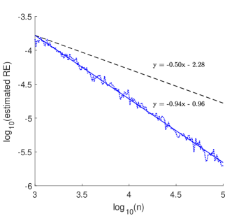
Figure 1: The relative error of estimator (2) for $\gamma=\mathbb{E}S=5\exp(1/2),d=5$, $\Sigma=\mathrm{I},\boldsymbol{\nu}=\boldsymbol{0}$. Also displayed is a reference line with the canonical slope of $-1/2$.

2.1 Density Estimator

To derive the smooth density estimator, we use the so-called push-out method (kroese2011handbook, , Chapter 11). In particular, observe that we can “push-out” $\gamma$ as follows:

$$\textstyle\ell(\gamma)=\mathbb{P}(\exp(\nu_{1}-\ln(\gamma)+L_{11}Z_{1})+\cdots+\exp(\nu_{d}-\ln(\gamma)+\sum_{j=1}^{d}L_{dj}Z_{j})\leq 1)$$

Therefore, the pdf of the SLN distribution can written as the integral:

$$\begin{split}f(\gamma)=\frac{\partial\ell}{\partial\gamma}&=\int_{\sum_{i}\exp(u_{i})<1}\frac{\partial}{\partial\gamma}\phi_{\Sigma}(\boldsymbol{u}-\boldsymbol{\nu}+\boldsymbol{1}\ln\gamma)\mathrm{d}\boldsymbol{u}\\ &=\int_{\sum_{i}\exp(u_{i})<1}\phi_{\Sigma}(\boldsymbol{u}-\boldsymbol{\nu}+\boldsymbol{1}\ln\gamma)\frac{-\boldsymbol{1}^{\top}\Sigma^{-1}(\boldsymbol{u}-\boldsymbol{\nu}+\boldsymbol{1}\ln\gamma)}{\gamma}\mathrm{d}\boldsymbol{u}\\ &=\int_{\sum_{i}\exp(u_{i})<\gamma}\phi_{\Sigma}(\boldsymbol{u}-\boldsymbol{\nu})\frac{-\boldsymbol{1}^{\top}\Sigma^{-1}(\boldsymbol{u}-\boldsymbol{\nu})}{\gamma}\mathrm{d}\boldsymbol{u}\\ &=\int_{\mathbb{R}^{d}}\phi(\boldsymbol{z})\frac{-\boldsymbol{z}^{\top}\mathrm{L}^{-1}\boldsymbol{1}}{\gamma}\textstyle\mathbb{I}\{\exp(\nu_{1}+L_{11}z_{1})+\cdots+\exp(\nu_{d}+\sum_{j=1}^{d}L_{dj}z_{j})<\gamma\}\mathrm{d}\boldsymbol{z}\end{split}$$

As a result of this, our smooth unbiased estimator of the SLN pdf is:

$$\hat{f}(\gamma)=\exp(\psi(\boldsymbol{Z};\boldsymbol{\mu}^{*}))\frac{-\boldsymbol{Z}^{\top}\mathrm{L}^{-1}\boldsymbol{1}}{\gamma},\qquad\boldsymbol{Z}\sim\mathbb{P}_{\boldsymbol{\mu}^{*}}$$ (4)

2.1.1 Numerical Examples

Using estimator (4), we can estimate accurately the effect of the correlation coefficient $\rho$ on the shape of the SLN pdf. The figure below shows that as $\rho$ increases the tail of the SLN pdf becomes thicker.

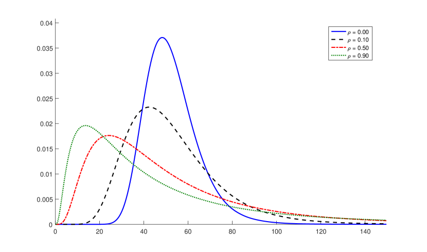
Figure 2: Estimate of the SLN pdf for $d=32,\boldsymbol{\nu}=\boldsymbol{0}$, $\Sigma=\rho\boldsymbol{1}\boldsymbol{1}^{\top}+(1-\rho)\mathrm{I}$, and varying $\rho$.

We now comment on what appears to be the only other viable Monte Carlo estimator of the SLN density.

The pdf estimator proposed in (asmussen2016exponential, , Equation 13) works only when the log-normal factors are independent, but one can extend it to the dependent case as shown in asmussen2017conditional . Let us denote the estimator proposed in asmussen2017conditional ; asmussen2016exponential by $\hat{\ell}_{\rm A}$. Tables 5 and 6 below compare the two estimators on two distinct numerical examples. The results suggest that (4) becomes significantly more efficient than $\hat{\ell}_{\rm A}$ when the $X_{i}$’s have different marginal distributions. Note that, as expected, the efficiency of (4) deteriorates as we approach the right tail (the right tail requires a different approach, see Section 3).

Table 5: The SLN distribution for $d=32,\boldsymbol{\nu}=\boldsymbol{0},\rho=0.5$, $\Sigma=\rho\boldsymbol{1}\boldsymbol{1}^{\top}+(1-\rho)\mathrm{I}$, using $n=10^{6}$ samples.

			relative error %		work normalized rel. var.
$\gamma$	$\hat{\ell}(\gamma)$	$\widehat{f}(\gamma)$	RE($\widehat{f}$)	RE($\widehat{f}_{{\rm A}}$)	WNRV($\widehat{f}$)	WNRV($\widehat{f}_{{\rm A}}$)
140	$0.957$	$9.12\text{\times}{10}^{-04}$	0.960	0.914	$7.93\text{\times}{10}^{-04}$	$1.50\text{\times}{10}^{-03}$
100	$0.894$	$2.53\text{\times}{10}^{-03}$	0.421	0.643	$1.52\text{\times}{10}^{-04}$	$7.42\text{\times}{10}^{-04}$
80	$0.826$	$4.46\text{\times}{10}^{-03}$	0.260	0.538	$5.84\text{\times}{10}^{-05}$	$5.05\text{\times}{10}^{-04}$
60	$0.705$	$7.96\text{\times}{10}^{-03}$	0.151	0.462	$2.00\text{\times}{10}^{-05}$	$3.61\text{\times}{10}^{-04}$
50	$0.613$	$1.06\text{\times}{10}^{-02}$	0.113	0.436	$1.14\text{\times}{10}^{-05}$	$3.23\text{\times}{10}^{-04}$
40	$0.490$	$1.38\text{\times}{10}^{-02}$	0.090	0.426	$7.05\text{\times}{10}^{-06}$	$3.08\text{\times}{10}^{-04}$
30	$0.336$	$1.69\text{\times}{10}^{-02}$	0.084	0.444	$6.23\text{\times}{10}^{-06}$	$3.31\text{\times}{10}^{-04}$
20	$0.163$	$1.71\text{\times}{10}^{-02}$	0.098	0.543	$8.70\text{\times}{10}^{-06}$	$4.94\text{\times}{10}^{-04}$
15	$0.831$	$1.41\text{\times}{10}^{-02}$	0.113	0.693	$1.17\text{\times}{10}^{-05}$	$7.99\text{\times}{10}^{-04}$

Table 6: The SLN distribution for $d=10,\rho=0$, $\nu_{i}=i-d$, $\sigma_{i}^{2}=i$, estimated with $n=10^{6}$ samples.

			relative error %		work normalized rel. var.
$\gamma$	$\hat{\ell}(\gamma)$	$\widehat{f}(\gamma)$	RE($\widehat{f}$)	RE($\widehat{f}_{{\rm A}}$)	WNRV($\widehat{f}$)	WNRV($\widehat{f}_{{\rm A}}$)
500	$0.964$	$5.28\text{\times}{10}^{-05}$	6.22	12.0	$1.09\text{\times}{10}^{-02}$	$2.60\text{\times}{10}^{-02}$
100	$0.881$	$8.01\text{\times}{10}^{-04}$	1.86	30.2	$9.91\text{\times}{10}^{-04}$	$1.66\text{\times}{10}^{-01}$
30	$0.746$	$4.81\text{\times}{10}^{-03}$	0.88	13.3	$2.08\text{\times}{10}^{-04}$	$3.23\text{\times}{10}^{-02}$
15	$0.633$	$1.21\text{\times}{10}^{-02}$	0.59	7.23	$9.56\text{\times}{10}^{-05}$	$9.52\text{\times}{10}^{-03}$
7	$0.484$	$2.96\text{\times}{10}^{-02}$	0.39	5.26	$4.26\text{\times}{10}^{-05}$	$5.05\text{\times}{10}^{-03}$
3	$0.310$	$6.58\text{\times}{10}^{-02}$	0.27	3.51	$2.09\text{\times}{10}^{-05}$	$2.22\text{\times}{10}^{-03}$
1	$0.125$	$1.29\text{\times}{10}^{-01}$	0.17	2.42	$8.86\text{\times}{10}^{-06}$	$1.03\text{\times}{10}^{-03}$
0.5	$0.0548$	$1.50\text{\times}{10}^{-01}$	0.14	2.24	$5.56\text{\times}{10}^{-06}$	$9.12\text{\times}{10}^{-04}$

Finally, we confirmed that, as expected, quasi Monte Carlo again accelerates the speed of convergence of the smooth estimator (4) by as much as approximately $\mathcal{O}(n^{-0.92})$. The qualitative behavior is depicted on Figure 3, where we also show the rate of convergence of its competitor $\hat{\ell}_{\rm A}$. Here, again, the relative error (in percent) is estimated using $100$ independent random shifts of Sobol’s quasirandom pointset (kroese2011handbook, , Section 2.5).

The reason that estimator (4) achieves a better convergence rate is that, while $\hat{\ell}_{\rm A}$ is continuous, but not differentiable, the estimator (4) is infinitely differentiable, and hence more amenable to acceleration with quasirandom sequences.

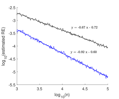
Figure 3: The relative error of estimator (2) (in blue with slope -0.92) for $\gamma=\mathbb{E}S=5\exp(1/2),d=5$, $\Sigma=\mathrm{I},\boldsymbol{\nu}=\boldsymbol{0}$, as well as that of $\hat{\ell}_{\rm A}$ (in red with slope -0.67).

2.2 Perfect Simulation from Conditional Distribution

One of advantages of our approach is that when $d$ is not too large, for the first time, it is possible to simulate exactly from the distribution of $\boldsymbol{X}$, conditional on the rare-event $\left\{\sum_{k=1}^{d}X_{k}\leq\gamma\right\}$. As $\psi(\boldsymbol{z};\boldsymbol{\mu}^{*})$ is concave in $\boldsymbol{z}$ for any fixed $\boldsymbol{\mu}^{*}$ (see, for example, (botev2017normal, Lemma 1)), we can easily obtain its maximum. This can then be used in the following acceptance-rejection sampling procedure.

1. Require: $c=\max_{\boldsymbol{z}}\psi(\boldsymbol{z};\boldsymbol{\mu}^{*})$

2. Until $E>c-\psi(\boldsymbol{Z};\boldsymbol{\mu}^{*})$ do
   Simulate $\boldsymbol{Z}\sim\mathbb{P}_{\boldsymbol{\mu}^{*}}$ and $E\sim{\sf Exp}(1)$, independently.

3. Return $\boldsymbol{X}=\exp(\boldsymbol{\nu}+\mathrm{L}\boldsymbol{Z})$ as a sample from the conditional distribution.

We next exploit the ability to simulate from the conditional SLN distribution to simulate exactly the stock price trajectories of an Asian option with positive payoff.

2.2.1 Exact Simulation of Stock Prices under Black-Scholes

We consider the average value of a stock price observed at a set of discrete times on the interval $[0,T]$,

$$\bar{X}_{T}=\frac{1}{d+1}\sum_{i=0}^{d}X_{t_{i}},\quad t_{0}=0<t_{1}<t_{2}<\cdots<t_{d}=T,$$

under the Black-Scholes model $X_{t}=X_{0}\exp\left((r-\sigma^{2}/2)t+\sigma W_{t}\right)$, where: (1) $W_{t}$ is the Wiener process at time $t$; (2) $\sigma$ is the volatility coefficient; (3) $r$ is the risk-free interest rate. Then, for an Asian Put option with maturity $T$ and strike price $K$ the payout is $(K-\bar{X}_{T})^{+}$. Since $\boldsymbol{X}=\left(X_{t_{1}},X_{t_{2}},\ldots,X_{t_{d}}\right)$ is a log-normal random vector with

$$\begin{split}&\nu_{i}=\ln(X_{0})+(r-\sigma^{2}/2)t_{i},\quad i=1,\ldots,d\\ &\Sigma_{ij}=\sigma^{2}\min\left(t_{i},t_{j}\right),\quad i,j=1,\ldots,d,\end{split}$$

we can use our algorithm above to simulate a realization of the stock price path conditional on the event $\{\bar{X}_{T}<K\}=\{X_{t_{1}}+\cdots+X_{t_{d}}<(d+1)K-X_{0}\}$. Simulation of such an $\boldsymbol{X}$ conditional on the rare-event $\{\bar{X}_{T}\leq 30\}$ provides insight into how the rare event occurs, that is, how the stock price must behave for a positive payoff.

The following figure shows one stock price realization with parameters $X_{0}=50,K=30,\sigma=0.25,r=0.07,T=4/12,d=88$.

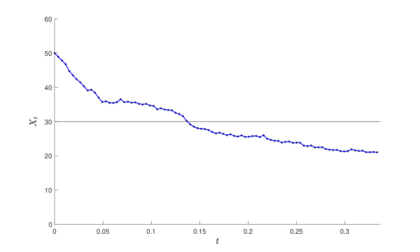
Figure 4: Stock price trajectory, conditional on $\bar{X}_{T}\leq 30$.

We note that, since $\mathbb{P}(\bar{X}_{T}\leq 30)\approx 2\times 10^{-11}$ is a rare-event probability, exact simulation of such a stock price trajectory is not possible using a naive acceptance-rejection, because the acceptance rate would be approximately $2\times 10^{-11}$. Instead, our algorithm enjoys the (estimated) acceptance rate of $5.9\%$.

3 Accurate Estimation of the Right Tail

In this section, we provide an estimator of the right tail of the SLN distribution, that is,

$$\mathbb{P}(X_{1}+\cdots+X_{d}\geq\gamma),\qquad\ln\boldsymbol{X}\sim\mathsf{N}(\boldsymbol{\nu},\Sigma)$$

that works well for many parameter settings for which all existing estimators fail. In order to keep the notation minimal, we recycle the notation for the left tail and henceforth let

$$\ell(\gamma)\stackrel{{\scriptstyle\mathrm{def}}}{{=}}\mathbb{P}(\exp(Y_{1})+\cdots\exp(Y_{d})\geq\gamma),\qquad\boldsymbol{Y}\sim\mathsf{N}(\boldsymbol{\nu},\Sigma)$$

Further, we set $S=X_{1}+\cdots+X_{d},M=\max_{i}X_{i}$, and $\sigma_{i}^{2}=\Sigma_{ii},\sigma=\max_{k}\sigma_{k},\nu=\max\{\nu_{k}:\sigma_{k}=\sigma\}$. Note that with all random variates defined on the same probability space, we can write $\boldsymbol{X}=\exp(\boldsymbol{Y})$.

One of the reasons why estimating the right tail is difficult is due to the heavy-tailed behavior of $\ell(\gamma)$ as $\gamma\uparrow\infty$ (see Corollary 1 here or asmussen2008asymptotics ):

$$\ell(\gamma)\simeq\ell_{\mathrm{as}}\stackrel{{\scriptstyle\mathrm{def}}}{{=}}\sum_{k=1}^{d}\mathbb{P}(Y_{i}\geq\ln\gamma)=\sum_{k=1}^{d}\overline{\Phi}((\ln\gamma-\nu_{k})/\sigma_{k})$$ (5)

To tackle this problem, the authors of asmussen2011efficient ; blanchet2008efficient ; gulisashvili2016tail ; kortschak2013efficient propose a number of theoretically efficient estimators. The problem with these estimators, however, is that their established theoretical efficiency does not necessarily translate into estimators with reasonably low Monte Carlo variance. Before proceeding to remedy this problem, we next explain why these existing proposals can fail to estimate $\ell(\gamma)$ — we provide both numerical evidence and theoretical insight.

3.1 Variance Boosted Estimator

We call the first estimator proposed in the literature the variance boosted estimator asmussen2011efficient ; blanchet2008efficient . It is defined as follows.

Let $\mathbb{P}_{\theta}$ be an importance sampling measure under which $\boldsymbol{Y}\sim\mathsf{N}(\boldsymbol{\nu},\Sigma/(1-\theta))$ for some parameter $\theta\in[0,1)$. If we take $\theta$ sufficiently close to unity, then we can inflate the variance of $\boldsymbol{Y}$ to induce the event $\{S>\gamma\}$. We thus obtain the variance boosted estimator:

$$\hat{\ell}_{\theta}(\gamma)=\frac{\exp(-\theta(\boldsymbol{Y}-\boldsymbol{\nu})^{\top}\Sigma^{-1}(\boldsymbol{Y}-\boldsymbol{\nu})/2)}{(1-\theta)^{d/2}}\mathbb{I}\{S>\gamma\},\qquad\boldsymbol{Y}\sim\mathbb{P}_{\theta}$$ (6)

One can choose $\theta$ optimally and show asmussen2011efficient that:

$$\frac{\mathbb{E}_{\theta}\hat{\ell}^{2}_{\theta}}{\ell^{2}}=\Theta([\ln\gamma]^{d/2+1}\gamma^{1/4})$$

Therefore, we expect that the variance boosted estimator will only be useful for very small $d$ and small $\gamma$. In contrast, in Section 3.3 we show that our new proposal has relative error which grows at the much slower rate of $\Theta(\ln\gamma)$.

Consider a simple example in which all log-normals are iid with $\sigma=0.25,\Sigma=\mathrm{I}\times\sigma^{2},\boldsymbol{\nu}=\boldsymbol{0},d=30$. Table 7 shows the estimated values for $\ell(\gamma)$ for different values of $\gamma$ using three different estimators: the variance boosted $\hat{\ell}_{\theta}$; the Asmussen-Kroese estimator asmussen2006improved ,

$$\textstyle\hat{\ell}_{\mathrm{AK}}=d\overline{\Phi}\left(\frac{1}{\sigma}\ln\left[(\gamma-\sum_{j<d}X_{j})\vee\max_{j<d}X_{j}\right]\right),\quad\ln\boldsymbol{X}\sim\mathsf{N}(\boldsymbol{0},\sigma^{2}\mathrm{I});$$ (7)

and our proposed estimator $\hat{\ell}$ in Section 3.3. The data was populated using $n=10^{7}$ independent replications of each estimator. The difference in the CPU run times for all methods was negligible (all between 7 to 10 seconds), and hence not reported here. The conclusion from the results in the table is that the variance boosted estimator, $\hat{\ell}_{\theta}$, is not useful due to its high variability.

Table 7: Comparative performance of the variance-boosted and Asmussen-Kroese estimators. The proposed estimator $\hat{\ell}$ is given in column two and described in Section 3.3.

			relative error %
$\gamma$	$\hat{\ell}$	$\hat{\ell}_{\mathrm{AK}}$	$\mathrm{RE}(\hat{\ell})$	$\mathrm{RE}(\hat{\ell}_{\mathrm{AK}})$	$\mathrm{RE}(\hat{\ell}_{\theta})$
30	0.74	0.74	0.199	0.0321	0.314
33	0.079	0.079	0.26	0.0871	3.67
36	0.00052	0.00052	0.403	0.684	39.8
39	$2.94\text{\times}{10}^{-07}$	$3.31\text{\times}{10}^{-07}$	0.725	17.9	51.9
42	$2.29\text{\times}{10}^{-11}$	$9.23\text{\times}{10}^{-14}$	1.45	54.6	99.9
45	$3.92\text{\times}{10}^{-16}$	$7.78\text{\times}{10}^{-20}$	2.57	64.4	97.8
48	$1.93\text{\times}{10}^{-21}$	$2.13\text{\times}{10}^{-25}$	4.44	31.7	97
51	$3.98\text{\times}{10}^{-27}$	$2.40\text{\times}{10}^{-29}$	7.85	25.2	81.5
54	$8.58\text{\times}{10}^{-33}$	$3.96\text{\times}{10}^{-33}$	3.22	15.3	100
57	$3.44\text{\times}{10}^{-36}$	$3.07\text{\times}{10}^{-36}$	0.418	13.3	69.8
60	$4.26\text{\times}{10}^{-39}$	$3.86\text{\times}{10}^{-39}$	0.203	5.21	99.7
63	$1.06\text{\times}{10}^{-41}$	$1.01\text{\times}{10}^{-41}$	0.18	2.92	99
66	$4.38\text{\times}{10}^{-44}$	$4.39\text{\times}{10}^{-44}$	0.162	1.58	64.8
69	$2.75\text{\times}{10}^{-46}$	$2.74\text{\times}{10}^{-46}$	0.16	1.09	100
72	$2.42\text{\times}{10}^{-48}$	$2.40\text{\times}{10}^{-48}$	0.155	0.686	98.3
75	$2.83\text{\times}{10}^{-50}$	$2.81\text{\times}{10}^{-50}$	0.153	0.498	72.1
78	$4.24\text{\times}{10}^{-52}$	$4.21\text{\times}{10}^{-52}$	0.151	0.414	95.7
81	$7.87\text{\times}{10}^{-54}$	$7.86\text{\times}{10}^{-54}$	0.15	0.287	99.3
84	$1.78\text{\times}{10}^{-55}$	$1.78\text{\times}{10}^{-55}$	0.15	0.26	100
87	$4.74\text{\times}{10}^{-57}$	$4.75\text{\times}{10}^{-57}$	0.15	0.251	90.5
90	$1.48\text{\times}{10}^{-58}$	$1.48\text{\times}{10}^{-58}$	0.15	0.189	100

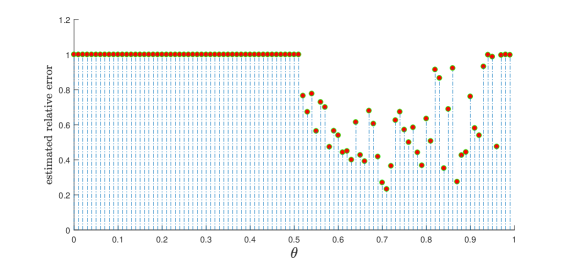
Figure 5: The estimated relative error of $\hat{\ell}_{\theta}$ as a function of $\theta$ using $10^{7}$ replications. The smallest estimated relative error was $23\%$, corresponding to $\theta=0.71$. Where the estimate of $\ell(45)$ is $0$, the relative error is recorded as unity (100%).

It is important to note that there is no value for $\theta$ that yields reasonably low variance. For example, Figure 5 shows the estimated relative error of $\hat{\ell}_{\theta}$ as a function of $\theta$ for $\gamma=45$ and all other parameters being the same as in Table 7. The figure suggests that even if we knew the true variance-minimizing $\theta^{*}$ (obviating the need for approximating it), the estimator will still not be useful.

3.2 Vanishing Relative Error Estimator

Recognizing the deficiency of the variance boosted estimator asmussen2011efficient ; blanchet2008efficient propose the superior importance sampling vanishing relative eror (ISVE) estimator. The main idea of the ISVE estimator is to split $\ell$ into two parts:

$$\ell=\mathbb{P}(M>\gamma)+\mathbb{P}(S>\gamma,M<\gamma),$$

and estimate $\ell_{1}=\mathbb{P}(M>\gamma)$ and $\ell_{2}=\mathbb{P}(S>\gamma,M<\gamma)$ separately using two different importance sampling schemes. In particular, $\ell_{1}$ is estimated via

$$\hat{\ell}_{1}=\frac{\ell_{\mathrm{as}}(\gamma)}{\sum_{k=1}^{d}\mathbb{I}\{X_{k}>\gamma\}},\quad\boldsymbol{X}\sim g(\boldsymbol{x}),$$ (8)

where $g$ is the mixture density:

$$g(\boldsymbol{x})\stackrel{{\scriptstyle\mathrm{def}}}{{=}}\frac{\phi_{\Sigma}(\boldsymbol{x}-\boldsymbol{\nu})\sum_{k=1}^{d}\mathbb{I}\{x_{k}>\gamma\}}{\ell_{\mathrm{as}}(\gamma)},$$ (9)

and the residual probability, $\ell_{2}$, is estimated via a variance boosted estimator:

$$\hat{\ell}_{2,\theta}(\gamma)=\frac{\exp(-\theta(\boldsymbol{Y}-\boldsymbol{\nu})^{\top}\Sigma^{-1}(\boldsymbol{Y}-\boldsymbol{\nu})/2)}{(1-\theta)^{d/2}}\mathbb{I}\{S>\gamma,M<\gamma\},\qquad\boldsymbol{Y}\sim\mathbb{P}_{\theta},$$ (10)

where $\theta=1-\Theta(\ln^{-2}(\gamma))$. With this setup the ISVE estimator is

$$\hat{\ell}_{\mathrm{ISVE}}=\hat{\ell}_{1}+\hat{\ell}_{2}$$

and it enjoys the vanishing relative error property asmussen2011efficient :

$$\frac{\mathbb{V}\mathrm{ar}(\hat{\ell}_{\mathrm{ISVE}})}{\ell^{2}(\gamma)}\downarrow 0,\quad\gamma\uparrow\infty.$$

Before we proceed to illustrate the practical performance of the ISVE estimator, we note that there are two issues that may indicate problematic performance.

First, in practical simulations one estimates the precision of an estimator $\hat{l}$ of $\ell$ by generating $n$ independent realizations, namely $\hat{l}_{1},\ldots,\hat{l}_{n}$, and then computing the corresponding sample variance $S_{n}^{2}=\frac{1}{n}\sum_{i=1}^{n}(\hat{l}_{i}-\bar{l})^{2},$ where $\bar{l}_{n}=(\hat{l}_{1}+\cdots+\hat{l}_{n})/n$. Ideally, $S_{n}/(\bar{l}_{n}\sqrt{n})$ would then yield a consistent estimator of the relative error of the sample mean and in numerical experiments we would report either the pair $\bar{l}_{n}$ and $S_{n}/(\bar{l}_{n}\sqrt{n})$, or (say) the 95% approximate confidence interval $\bar{l}_{n}\pm 1.96\times S_{n}/\sqrt{n}$. Unfortunately, these simple precision estimates cannot be applied to the $\hat{\ell}_{\mathrm{ISVE}}$ estimator, because the sample variance of $n$ independent replications of (8) is not a robust estimator of the true variance of $\hat{\ell}_{1}$. This is formalized in the following result, proved in the Appendix.

Lemma 1 (Inefficiency of Sample Variance)

Let $S_{n}^{2}$ be the sample variance based on $n$ independent replications of (8) . Then, $S_{n}^{2}$ is not a logarithmically efficient estimator:

$$\limsup_{\gamma\uparrow\infty}\frac{\ln\mathbb{V}\mathrm{ar}(S_{n}^{2})}{\ln\mathbb{V}\mathrm{ar}(\hat{\ell}_{1})}<2,$$

so that the relative error in estimating the precision of $\hat{\ell}_{\mathrm{ISVE}}$ grows at an exponential rate in $\ln^{2}(\gamma)$.

One practical consequence of the result above is that the relative error of $\hat{\ell}_{\mathrm{ISVE}}$ is severely underestimated during simulation, and frequently reported as being zero. In contrast to this negative result for the ISVE estimator, in Corollary 2 we show that our new estimator enjoys an asymptotically efficient estimator of its true variability. Even better, estimation of the precision of our estimator is not more difficult than estimating $\ell$ itself.

A second problematic issue is that, as we have already seen, the variance boosted estimator (6) is unreliable for estimating $\ell$, and that there is no value for $\theta$ that will render it a useful estimator. Since (10) only differs from (6) with the addition of the constraint $M<\gamma$ and in the different choice of $\theta$, we should not be surprised to find that (10) is also a poor estimator of $\ell_{2}=\mathbb{P}(S>\gamma,M<\gamma)$. Indeed, there is no good value for $\theta$ that can make the relative error of (10) small. The behavior of the relative error of $\hat{\ell}_{2,\theta}$ as a function of $\theta$ is qualitatively the same as that on Figure 5.

3.2.1 Quality of Asymptotic Approximation

One of the arguments in favor of the ISVE estimator is that, while $\hat{\ell}_{2}$ may be a noisy estimator, it is a very small second order residual term, and will not affect noticeably the high accuracy of the leading order term $\hat{\ell}_{1}$.

Unfortunately, unless one considers extremely small probabilities, the leading contribution term of $\ell=\ell_{1}+\ell_{2}$ is not $\ell_{1}$, but the residual $\ell_{2}$. This does not contradict the fact that asymptotically $\ell\simeq\ell_{1}$, because in the presence of a positive correlation $\ell_{1}$, or equivalently $\ell_{\mathrm{as}}$, can be an extremely poor approximation to $\ell$.

Table 8: Illustration of the inaccuracy of the asymptotic approximation for moderate values of $\ell(\gamma)$. The asymptotic approximation $\ell_{\mathrm{as}}$ becomes useful only for probabilities smaller than about $10^{-233}$.

$\gamma$	$\ell_{\mathrm{as}}$	95% CI for $\hat{\ell}$	$(\hat{\ell}-\ell_{\mathrm{as}})/\ell_{\mathrm{as}}$
$15$	$1.2113\ldots\times 10^{-26}$	$0.012\pm 0.001$	$1.0\times 10^{24}$
$20$	$2.1830\ldots\times 10^{-32}$	$(5.80\pm 0.013)\times 10^{-5}$	$2.66\times 10^{27}$
$40$	$1.4175\ldots\times 10^{-48}$	$(6.33\pm 0.016)\times 10^{-15}$	$4.5\times 10^{33}$
$60$	$1.3872\ldots\times 10^{-59}$	$(1.10\pm 0.017)\times 10^{-23}$	$8\times 10^{35}$
$100$	$4.4834\ldots\times 10^{-75}$	$(8.04\pm.018)\times 10^{-38}$	$1.8\times 10^{37}$
$500$	$1.0481\ldots\times 10^{-135}$	$(3.39\pm.02)\times 10^{-105}$	$3.2\times 10^{30}$
$1000$	$2.3594\ldots\times 10^{-167}$	$(6.94\pm.02)\times 10^{-145}$	$3\times 10^{22}$
$1500$	$2.0634\ldots\times 10^{-187}$	$(4.04\pm.03)\times 10^{-171}$	$2\times 10^{16}$
$2500$	$2.6294\ldots\times 10^{-214}$	$(2.94\pm.04)\times 10^{-207}$	$1.1\times 10^{7}$
$3500$	$5.1912\ldots\times 10^{-233}$	$(5.45\pm.04)\times 10^{-233}$	$0.05$

To illustrate the quality of the asymptotic approximation take the instances in Table 8, where $d=10$ and $\boldsymbol{\nu}=\boldsymbol{0},\Sigma=0.25^{2}\times(0.9\times\boldsymbol{1}\boldsymbol{1}^{\top}+(1-0.9)\times\mathrm{I})$. The table shows the asymptotic value $\ell_{\mathrm{as}}$ for different $\gamma$ (second column), together with its relative deviation from the true $\ell$ (last column). The table also displays $\hat{\ell}$ with its approximate 95% confidence interval based on $n=10^{6}$ independent replications of our method in Section 3.3.

We conclude from Table 8 that the asymptotic approximation is useless for moderate values of $\gamma$ (deviating from the true value of $\ell$ by as much as $10^{37}$), and only becomes useful for extremely small probabilities (smaller than $10^{-233}$).

In fact, for the numerical experiment above it can be shown (see kortschak2014second ) that the second order asymptotic term is:

$$\begin{split}\ell(\gamma)-\ell_{\mathrm{as}}(\gamma)&=\ell(\gamma)-d\overline{\Phi}(\ln\gamma)\simeq d(d-1)\exp((1-\rho^{2})/2)\frac{\ln(\gamma)}{\gamma^{1-\rho}}\overline{\Phi}(\ln\gamma)\end{split}$$

In other words, the relative error of the asymptotic approximation,

$$\frac{\ell(\gamma)-\ell_{\mathrm{as}}(\gamma)}{\ell_{\mathrm{as}}(\gamma)}=\Theta\left(\frac{\ln\gamma}{\gamma^{1-\rho}}\right),$$

decays at a polynomial rate, and this rate can be extremely slow when $\rho$ is close to unity. Even worse, with $\rho=0.99$ the term $\frac{\ln\gamma}{\gamma^{1-\rho}}$ increases as a function of $\gamma$ for values up to $\gamma\leq\exp(1/(1-\rho))=\exp(100)\approx 10^{43}$, and only starts decaying to zero for $\gamma>\exp(100)$.

3.3 Exponentially Tilted Estimator

Given the failure of the estimators described above, a natural question arises. What kind of estimator will succeed in being both theoretically efficient and exhibit low variance in practical simulations?

To answer this question we start by examining the quite natural proposal of Gulisashvili and Tankov (GT) (gulisashvili2016tail, , Equation (70)), which can be written as follows:

$$\hat{\ell}_{\mathrm{GT}}\stackrel{{\scriptstyle\mathrm{def}}}{{=}}\exp\left(\frac{\boldsymbol{\mu}^{\top}\Sigma^{-1}\boldsymbol{\mu}}{2}-\boldsymbol{\mu}^{\top}\Sigma^{-1}(\boldsymbol{Y}-\boldsymbol{\nu})\right)\mathbb{I}\{S\geq\gamma\},\qquad\boldsymbol{Y}\sim\mathsf{N}(\boldsymbol{\mu}+\boldsymbol{\nu},\Sigma),$$ (11)

where the parameter $\boldsymbol{\mu}$ is chosen by minimizing an asymptotic approximation to the second moment (gulisashvili2016tail, , Equation (71)).

Unfortunately, (11) also performs poorly, just like the estimators in the last section. This poor practical performance is compounded by the fact that there is no proof of the asymptotic efficiency of (11) as $\gamma\uparrow\infty$ (see (gulisashvili2016tail, , Page 40)).

The reason why the estimator (11) performs poorly is that it uses a single exponential tilting parameter $\boldsymbol{\mu}$, which is insufficient to induce the mutually-exclusive mode of occurrence of the rare-event: $\mathbb{P}(X_{k}=M|S>\gamma)\simeq\frac{\mathbb{P}(X_{k}>\gamma)}{\ell}$ (see part 1 of Lemma 2). In other words, with asymptotic probability $\mathbb{P}(X_{k}>M)/\ell$, each $X_{k}$ is the maximal term that causes the sum to up-cross $\gamma$, and the single exponential tilting parameter $\boldsymbol{\mu}$ in (11) cannot account for this mutually-exclusive behavior.

Instead, to obtain a provably efficient estimator with excellent practical and theoretical performance, we must introduce $d$ distinct exponential tilting parameter vectors $\boldsymbol{\mu}_{1},\ldots,\boldsymbol{\mu}_{d}$, where each $\boldsymbol{\mu}_{k}$ is tasked to deal with the event $\{S>\gamma,X_{k}=M\}$. The new set of $d$ tilting parameters are also determined using an error estimate different from the one used in (11) when we have a single tilting parameter. Thus, our proposal uses an estimator of the form (11) for each term, $\hbar_{i}(\gamma)$, in the decomposition:

$$\ell(\gamma)=\sum_{i=1}^{d}\underbrace{\mathbb{P}(S>\gamma,X_{i}=M)}_{\hbar_{i}(\gamma)}.$$

The estimator of each $\hbar_{k}$ based on one replication is

$$\hat{\hbar}_{k}(\gamma)=\exp\left(\frac{\boldsymbol{\mu}_{k}^{\top}\Sigma^{-1}\boldsymbol{\mu}_{k}}{2}-\boldsymbol{\mu}_{k}^{\top}\Sigma^{-1}(\boldsymbol{Y}-\boldsymbol{\nu})\right)\mathbb{I}\{S>\gamma,X_{k}=M\},$$ (12)

where under the measure $\mathbb{P}_{\boldsymbol{\mu}_{k}}$ with expectation $\mathbb{E}_{\boldsymbol{\mu}_{k}}$ we have $\ln\boldsymbol{X}=\boldsymbol{Y}\sim\mathsf{N}(\boldsymbol{\nu}+\boldsymbol{\mu}_{k},\Sigma)$, and $\boldsymbol{\mu}_{k}$ is the solution to the non-linear optimization:

$$\begin{split}\min_{\boldsymbol{\mu}}\;\frac{1}{2}\boldsymbol{\mu}^{\top}\Sigma^{-1}\boldsymbol{\mu},\quad\textrm{subject to:}&\\ \textstyle g_{1}(\boldsymbol{\mu})=\exp(\mu_{k}+\nu_{k})+\sum_{i\not=k}\exp(\mu_{i}+\nu_{i}+\frac{\sigma_{i}^{2}}{2})-\gamma&\geq 0\\ \textstyle g_{2}(\boldsymbol{\mu})=\mu_{k}+\nu_{k}+\frac{\sigma_{k}^{2}}{2}-\max_{j\not=k}\{\mu_{j}+\nu_{j}+\frac{\sigma_{j}^{2}}{2}\}&\geq 0\end{split}$$ (13)

To construct the overall estimator $\hat{\ell}$ of $\ell$, we can use stratification with a total computing budget of $n=n_{1}+\cdots+n_{d}$ replications, whereby we allocate $n_{k}$ samples to estimate each $\hbar_{k}$ independently. We then take the sum of the estimators of $\hbar_{k}$’s as our stratified estimator of $\ell$. In other words,

$$\hat{\ell}(\gamma)=\sum_{k=1}^{d}\frac{1}{n_{k}}\sum_{j=1}^{n_{k}}\hat{\hbar}_{k,j}(\gamma),$$ (14)

where $\sum_{k}n_{k}=n$ and $\hat{\hbar}_{k,1},\ldots,\hat{\hbar}_{k,n_{k}}$ are iid copies of (12). We then have the following efficiency result.

Theorem 3 (Logarithmic Efficiency)

Suppose we select the stratified allocation such that $n_{i}\varpropto n\times\mathbb{P}(X_{i}>\gamma)$. Then, the estimator (14) is unbiased and logarithmically efficient with relative error $\mathbb{V}\mathrm{ar}(\hat{\ell}(\gamma))/\ell^{2}(\gamma)=\mathcal{O}(\ln\gamma)$ as $\gamma\uparrow\infty$.

Proof

First note that choosing $n_{k}=n\times\mathbb{P}(X_{k}>\gamma)/\ell_{\mathrm{as}}$ satisfies the constraint $n=\sum_{k}n_{k}$, but is in conflict with the constraint that the $n_{k}$’s have to be integers. One simple solution is to simply round up to the nearest integer, and violate the constraint $n=\sum_{k}n_{k}$. For large enough $n$, the residual $n-\sum_{k}n_{k}$ will be negligible. Another solution, which we adopt in our computer implementation, is to use a widely-used randomized stratification scheme, as described in, for example, (kroese2011handbook, , Algorithm 14.2).

Next, with the above allocation for each $n_{k}$, the variance of the stratified estimator (14) is:

$$\mathbb{V}\mathrm{ar}(\hat{\ell})=\frac{1}{n}\sum_{k=1}^{d}\frac{n}{n_{k}}\mathbb{V}\mathrm{ar}(\hat{\hbar}_{k})=\frac{\ell_{\mathrm{as}}}{n}\sum_{k=1}^{d}\frac{\mathbb{V}\mathrm{ar}(\hat{\hbar}_{k})}{\mathbb{P}(X_{k}>\gamma)}$$

Therefore, using the result 3. in Lemma 2, the relative error of $\hat{\ell}$ as $\gamma\uparrow\infty$ is

$$\begin{split}\frac{n\mathbb{V}\mathrm{ar}(\hat{\ell}(\gamma))}{\ell^{2}(\gamma)}&\simeq\frac{n\mathbb{V}\mathrm{ar}(\hat{\ell}(\gamma))}{\ell^{2}_{\mathrm{as}}(\gamma)}=\frac{1}{\ell_{\mathrm{as}}(\gamma)}\sum_{k=1}^{d}\mathbb{P}(X_{k}>\gamma)\frac{\mathbb{V}\mathrm{ar}(\hat{\hbar}_{k})}{[\mathbb{P}(X_{k}>\gamma)]^{2}}=\mathcal{O}(\ln\gamma).\end{split}$$ (15)

The last equation shows that $\frac{\ln\mathbb{V}\mathrm{ar}(\hat{\ell}^{2}(\gamma))}{\ln\ell(\gamma)}\rightarrow 2$ as $\gamma\uparrow\infty$.

We can now see that the rate of growth of the relative error of our estimator, namely $\mathcal{O}(\ln\gamma)$, is significantly slower than the rate of growth of the variance boosted estimator, $\mathcal{O}([\ln\gamma]^{d/2+1}\gamma^{1/4})$.

Since the proof of the following lemma is long, it is delegated to the appendix.

Lemma 2 (Asymptotics for $\hat{\hbar}_{k}$)

As $\gamma\uparrow\infty$, we have that:

1. $\mathbb{E}_{\boldsymbol{\mu}}[\hat{\hbar}_{k}(\gamma)]=\mathbb{P}(S>\gamma,X_{k}=M)\simeq\mathbb{P}(X_{k}>\gamma).$

2. The asymptotic solution to (13) is

   $$\boldsymbol{\mu}^{*}=\frac{\ln(\gamma)-\nu_{k}}{\sigma_{k}^{2}}\Sigma\boldsymbol{e}_{k},$$

   where $\boldsymbol{e}_{k}$ is the unit vector with $1$ in the $k$-th position.

3. We have $\frac{\mathbb{V}\mathrm{ar}(\hat{\hbar}_{k})}{[\mathbb{P}(X_{k}>\gamma)]^{2}}=\mathcal{O}(\ln\gamma)$, and with $\boldsymbol{\mu}$ solving (13) the $(m+1)$-st moment satisfies:

   $$\mathbb{E}_{\boldsymbol{\mu}}\hat{\hbar}^{m+1}_{k}=\Theta(\ln^{m}(\gamma)\hbar_{k}^{m+1})$$ (16)

Note that part 1. of the above lemma immediately yields the following corollary, which was originally proved in asmussen2008asymptotics using a different argument.

Corollary 1 (Right-Tail Asymptotics)

$\ell(\gamma)\simeq\sum_{i=1}^{d}\mathbb{P}(X_{k}>\gamma)$ as $\gamma\uparrow\infty$.

More importantly, part 3. of Lemma 2 gives us a robustness guarantee that is not enjoyed by any of the competing estimators.

Corollary 2 (Logarithmically Efficient Variance Estimator)

Let $S_{n_{k}}^{2}$ be the sample variance based on $n_{k}$ independent replications of (12). Then, $S_{n}^{2}$ is a logarithmically efficient estimator:

$$\liminf_{\gamma\uparrow\infty}\frac{\ln\mathbb{V}\mathrm{ar}(S_{n_{k}}^{2})}{\ln\mathbb{V}\mathrm{ar}(\hat{\hbar}_{k})}=2,$$

where the rate of growth is $\frac{\mathbb{V}\mathrm{ar}(S_{n_{k}}^{2})}{\mathbb{V}\mathrm{ar}^{2}(\hat{\hbar}_{k})}=\mathcal{O}(\ln\gamma)$.

Proof

Using (16), consider the following calculations:

$$\begin{split}\frac{n_{k}\mathbb{V}\mathrm{ar}(S_{n_{k}}^{2})}{\mathbb{V}\mathrm{ar}^{2}(\hat{\hbar}_{k})}&=\frac{\mathbb{E}_{\boldsymbol{\mu}}(\hat{\hbar}_{k}(\gamma)-\hbar_{k}(\gamma))^{4}}{[\mathbb{E}_{\boldsymbol{\mu}}(\hat{\hbar}_{k}(\gamma)-\hbar_{k}(\gamma))^{2}]^{2}}-1+\frac{2}{n_{k}-1}\\ &=\frac{\Theta(\ln^{3}(\gamma)\hbar_{k}^{4})+\hbar_{k}^{4}+\hbar_{k}^{2}\Theta(\ln(\gamma)\hbar_{k}^{2})-\hbar_{k}\Theta(\ln^{2}(\gamma)\hbar_{k}^{3})-4\hbar^{4}_{k}}{[\Theta(\ln(\gamma)\hbar_{k}^{2})-\hbar_{k}^{2}]^{2}}-1+\frac{2}{n_{k}-1}\\ &=\frac{\Theta(\ln^{3}\gamma)+\Theta(\ln\gamma)-\Theta(\ln^{2}\gamma)-3}{[\Theta(\ln\gamma)-1]^{2}}-1+\frac{2}{n_{k}-1}\\ &=\Theta(\ln(\gamma))-1+\frac{2}{n_{k}-1}\end{split}$$

Therefore, a major advantage of our proposed estimator (14) is that estimating its variance is asymptotically not more difficult than estimating $\ell$ itself.

In retrospect, we can see that the excellent theoretical properties of our estimator are due mainly to the breaking of the symmetry in the sum $S=X_{1}+\cdots+X_{d}$ by distinguishing each and every $X_{i}$ as the overall maximum. In contrast, the poorly performing estimators (11) and (10) (and hence $\hat{\ell}_{\mathrm{ISVE}}$) both induce a simple change of measure that does not conform to the mutually-exclusive asymptotic behavior of $\mathbb{P}(S>\gamma,X_{k}=M)\simeq\mathbb{P}(X_{k}>\gamma),\;k=1,\ldots,d$.

Finally, we remark on the unusual way of selecting $\boldsymbol{\mu}$ via the optimization (13). Why do we not simply use the asymptotic approximation $\boldsymbol{\mu}^{*}$ in Lemma 2? The answer is that, while asymptotically the matrix $\Sigma$ is irrelevant, it is still relevant for very large values of $\gamma$, and our change of measure should reflect this dependence. The asymptotic solution $\boldsymbol{\mu}^{*}$ does not reflect this dependence. Thus, (13) was designed with two objectives in mind: (1) good practical performance for finite $\gamma<\infty$, where the full $\Sigma$ is relevant; (2) asymptotic optimality as $\gamma\uparrow\infty$, where $\Sigma$ is irrelevant. The optimization program (13) transitions from objective (1) to objective (2) in a continuous way.

3.4 Numerical Comparison

In this section we show that the superior theoretical properties of (14) convert into excellent practical performance. In fact, the numerical simulations suggest that our proposed estimator is the only one capable of estimating $\ell$ in many settings of practical interest.

3.4.1 Comparison with ISVE estimator

Consider estimating $\ell(\gamma)$ with

$$d=30,\rho=0.9,\;\boldsymbol{\nu}=\boldsymbol{0},\;\Sigma=0.25^{2}\times(\rho\times\boldsymbol{1}\boldsymbol{1}^{\top}+(1-\rho)\times\mathrm{I})$$

and different values of $\gamma$. Table 9 gives the results using $n=10^{6}$ replications. For the ISVE estimator we attempted to optimize the performance of the estimator by manually selecting the best possible $\theta$. Our choice for this tuning parameter is thus given in brackets in the third column.

Table 9: Comparative performance of the ISVE and exponentially tilted estimators with $\rho=0.9$.

			relative error %		work normalized rel. var.
$\gamma$	$\hat{\ell}$	$\hat{\ell}_{\mathrm{ISVE}}$	$\mathrm{RE}(\hat{\ell})$	$\mathrm{RE}(\hat{\ell}_{\mathrm{ISVE}})$	$\mathrm{WNRV}(\hat{\ell})$	$\mathrm{WNRV}(\hat{\ell}_{\mathrm{ISVE}})$
40	0.116	0.114 ($\theta=0.5$)	0.63	2.0	0.00032	0.00080
100	$2.17\times 10^{-7}$	$1.18\times 10^{-7}$ ($\theta=0.6$)	0.98	40	0.00061	0.31
150	$6.83\times 10^{-12}$	$5.75\times 10^{-13}$ ($\theta=0.75$)	1.1	84	0.00093	1.12
200	$7.75\times 10^{-16}$	$2.09\times 10^{-17}$ ($\theta=0.8$)	1.2	95	0.0010	1.22
400	$6.57\times 10^{-28}$	$3.08\times 10^{-39}$ ($\theta=0.9$)	1.4	80	0.0011	1.34
$10^{3}$	$1.61\times 10^{-49}$	$1.21\times 10^{-80}$ ($\theta=0.95$)	1.7	100	0.002	2.02
$10^{4}$	$3.60\times 10^{-132}$	$1.80\times 10^{-294}$ ($\theta=?$)	2.1	-	0.0024	-

A number of conclusions can be drawn from the table.

First, the ISVE estimator does not have acceptably low variance for both small $\gamma$ (when the event is not rare) and for large $\gamma$ (when the event is rare).

Second, as with Figure 5, any attempt to optimize with respect to $\theta$ is fruitless, because there appears to be no value for $\theta\in[0,1)$ that yields low variance.

Third, in the last row of the table, it was not possible to induce the event $\{S>\gamma,M<\gamma\}$ no matter what the value of $\theta$. In other words, $\{S>\gamma,M<\gamma\}$ remains a rare-event for all values of $\theta\in[0,1)$, and with very high probability $\hat{\ell}_{\mathrm{ISVE}}=\hat{\ell}_{1}+\hat{\ell}_{2}=\hat{\ell}_{1}$. Thus, despite the vanishing relative error property of the ISVE estimator, its performance deteriorates as $\gamma$ becomes smaller and smaller to the point that it does not deliver meaningful estimates.

The next example in Table 10 suggests that our estimator remains robust even in very high dimensions of up to $d=60$.

Table 10: Performance for $d=60$, $n=10^{6}$, $\boldsymbol{\nu}=\boldsymbol{0}$, $\Sigma=0.5\times\boldsymbol{1}\boldsymbol{1}^{\top}+0.5\times\mathrm{I}$.

			relative error %		work normalized rel. var.
$\gamma$	$\widehat{\ell}$	$\widehat{\ell}_{\rm ISVE}$	${\rm RE}(\widehat{\ell})$	${\rm RE}(\widehat{\ell}_{\rm ISVE})$	WNRV$(\widehat{\ell})$	WNRV$(\widehat{\ell}_{\rm ISVE})$
600	$1.98\text{\times}{10}^{-03}$	$5.77\text{\times}{10}^{-07}$	$0.837$	$51.6$	$1.02\text{\times}{10}^{-03}$	$4.88\text{\times}{10}^{00}$
900	$2.81\text{\times}{10}^{-04}$	$4.00\text{\times}{10}^{-10}$	$0.893$	$15.4$	$1.20\text{\times}{10}^{-03}$	$4.42\text{\times}{10}^{-01}$
1200	$5.91\text{\times}{10}^{-05}$	$4.16\text{\times}{10}^{-11}$	$0.93$	$3.16$	$1.36\text{\times}{10}^{-03}$	$1.75\text{\times}{10}^{-02}$
1500	$1.57\text{\times}{10}^{-05}$	$7.92\text{\times}{10}^{-12}$	$0.964$	$1.23$	$1.52\text{\times}{10}^{-03}$	$2.56\text{\times}{10}^{-03}$
1800	$5.01\text{\times}{10}^{-06}$	$2.01\text{\times}{10}^{-12}$	$0.987$	$1.50$	$1.57\text{\times}{10}^{-03}$	$3.41\text{\times}{10}^{-03}$
2100	$1.79\text{\times}{10}^{-06}$	$6.05\text{\times}{10}^{-13}$	$1.012$	$0.0543$	$2.03\text{\times}{10}^{-03}$	$5.10\text{\times}{10}^{-06}$
2400	$7.18\text{\times}{10}^{-07}$	$2.12\text{\times}{10}^{-13}$	$1.029$	$2.84\text{\times}{10}^{-03}$	$1.56\text{\times}{10}^{-03}$	$1.11\text{\times}{10}^{-08}$
2700	$3.08\text{\times}{10}^{-07}$	$8.30\text{\times}{10}^{-14}$	$1.046$	$8.93\text{\times}{10}^{-04}$	$1.63\text{\times}{10}^{-03}$	$1.15\text{\times}{10}^{-09}$
3000	$1.44\text{\times}{10}^{-07}$	$3.54\text{\times}{10}^{-14}$	$1.057$	$6.82\text{\times}{10}^{-04}$	$2.02\text{\times}{10}^{-03}$	$5.97\text{\times}{10}^{-10}$
3300	$7.02\text{\times}{10}^{-08}$	$1.63\text{\times}{10}^{-14}$	$1.069$	$8.30\text{\times}{10}^{-04}$	$2.05\text{\times}{10}^{-03}$	$9.60\text{\times}{10}^{-10}$

3.4.2 Comparison with Modified Asmussen-Kroese estimator

In addition to the ISVE estimator, the modified Asmussen-Kroese (MAK) estimator (kortschak2013efficient, , Equation 3.6) also enjoys the vanishing relative error property. In comparing (14) with the MAK estimator, we make the following observations.

First, the MAK estimator requires the solution of a non-linear equation for every replication. This aspect of the estimator poses nontrivial problems: (1) sometimes no solution exists; (2) Newton’s method may take many iterations to converge, making the running time of the estimator large.

Second, while our estimator (14) was shown to be second-order efficient, ensuring reliable estimation of its precision, no such efficiency result is provided for the MAK estimator, and in numerical experiments we sometimes observed significant underestimation of the true variance of the MAK estimator.

Third, observe that the MAK estimator reduces to the Asmussen-Kroese (AK) estimator (7) in the independent case: $\boldsymbol{\nu}=\nu\boldsymbol{1},\Sigma=\sigma^{2}\mathrm{I}$. Table 7 shows that when $\sigma$ is small our estimator can outperform the (modified) Asmussen-Kroese estimator by orders of magnitude. For example, note how for $\gamma\in[42,51]$ the AK estimator severely underestimates the true probability by as much as an order of $10^{-4}$. Interestingly, the Asmussen-Kroese estimator has superior and unrivaled performance only in cases with larger $\sigma$, say $\sigma\geq 1$.

Finally, Table 11 below confirms that the MAK estimator inherits the poor performance of the Asmussen-Kroese estimator for small $\sigma$. In this particular example we use

$$d=10,\;\boldsymbol{\nu}=\boldsymbol{0},\;\rho=0.2,\;\Sigma=0.25^{2}(\rho\boldsymbol{1}\boldsymbol{1}^{\top}+(1-\rho)\mathrm{I}).$$

Observe how for $\gamma\in[26,30]$ the MAK estimator underestimates the true probability by as much as an order of $10^{-3}$.

Table 11: Comparative performance for $d=10,n=10^{6},\boldsymbol{\nu}=\boldsymbol{0},\rho=0.2,\Sigma=0.25^{2}(\rho\boldsymbol{1}\boldsymbol{1}^{\top}+(1-\rho)\mathrm{I})$.

			relative error %		work normalized rel. var.
$\gamma$	$\hat{\ell}_{\mathrm{MAK}}$	$\hat{\ell}$	$\mathrm{RE}(\hat{\ell}_{\mathrm{MAK}})$	$\mathrm{RE}(\hat{\ell})$	$\mathrm{WNRV}(\hat{\ell}_{\mathrm{MAK}})$	$\mathrm{WNRV}(\hat{\ell})$
15	0.00195	0.00198	0.420	0.669	0.00531	$4.15\text{\times}{10}^{-05}$
16	0.000373	0.000370	0.660	0.724	0.0130	$5.03\text{\times}{10}^{-05}$
17	$6.47\text{\times}{10}^{-05}$	$6.47\text{\times}{10}^{-05}$	1.07	0.775	0.0349	$5.20\text{\times}{10}^{-05}$
18	$1.00\text{\times}{10}^{-05}$	$1.02\text{\times}{10}^{-05}$	1.80	0.823	0.096	0.000102
19	$1.57\text{\times}{10}^{-06}$	$1.52\text{\times}{10}^{-06}$	3.10	0.87	0.28	$6.71\text{\times}{10}^{-05}$
20	$2.02\text{\times}{10}^{-07}$	$2.15\text{\times}{10}^{-07}$	5.60	0.937	0.941	$8.09\text{\times}{10}^{-05}$
21	$3.11\text{\times}{10}^{-08}$	$2.99\text{\times}{10}^{-08}$	9.2	1.00	2.56	0.000166
22	$3.80\text{\times}{10}^{-09}$	$3.91\text{\times}{10}^{-09}$	15.9	1.06	7.58	0.000108
23	$3.22\text{\times}{10}^{-10}$	$5.15\text{\times}{10}^{-10}$	19.0	1.07	11.2	0.000327
24	$5.63\text{\times}{10}^{-11}$	$6.61\text{\times}{10}^{-11}$	44.7	1.14	61.57	0.000123
25	$6.09\text{\times}{10}^{-12}$	$8.42\text{\times}{10}^{-12}$	42.0	1.18	55.0	0.00036
26	$4.63\text{\times}{10}^{-13}$	$1.05\text{\times}{10}^{-12}$	71.6	1.23	159	0.000197
27	$1.90\text{\times}{10}^{-14}$	$1.33\text{\times}{10}^{-13}$	31.5	1.40	30.0	0.000176
28	$4.85\text{\times}{10}^{-15}$	$1.69\text{\times}{10}^{-14}$	60.0	1.49	110.	0.000187
29	$9.12\text{\times}{10}^{-17}$	$2.15\text{\times}{10}^{-15}$	60.4	1.5	113.34	0.00021378
30	$6.37\text{\times}{10}^{-18}$	$2.74\text{\times}{10}^{-16}$	53.1	1.54	87.585	0.00018874

4 Conclusions

We have presented new methodology for the accurate estimation of the cdf, pdf, and tails of the SLN distribution. In all three cases the new methodology yields estimators that can tackle parameter settings which are currently intractable with existing methods. In the cdf and pdf cases, the proposed estimators permit additional variance reduction via Quasi Monte Carlo. In the right-tail case, the new exponentially tilted estimator is shown to be, not only logarithmically or weakly efficient, but also second-order efficient. This permits us to have greater confidence in all error estimates derived from simulation.

One of the crucial observations we can draw from a number of numerical experiments is that sometimes a strongly efficient estimator ($\hat{\ell}_{\mathrm{ISVE}},\hat{\ell}_{\mathrm{MAK}}$) may not necessarily exhibit low variance in practical simulations, and may be bettered by a much simpler weakly efficient estimator.

In subsequent work, we will explore using the sequential sampling ideas in Section 2 for the estimation of the distribution of an iid sum of random variables with an arbitrary (be it light- or heavy-tailed) distribution.

Appendix

Proof of Theorem 1

Proof

Under the assumption that $\Sigma_{11}<\Sigma_{1j}$ for $j\not=1$, we have $\ell(\gamma)\simeq\mathbb{P}(X_{1}<\gamma)$, see gulisashvili2016tail for a proof. Therefore, using the upper bound

$$\mathbb{E}_{\boldsymbol{0}}\hat{\ell}^{2}_{\boldsymbol{0}}(\gamma)=\mathbb{E}_{\boldsymbol{0}}\prod_{j=1}^{d}\Phi^{2}(\alpha_{j}(Z_{1},\ldots,Z_{j-1}))\leq\mathbb{E}\Phi^{2}(\alpha_{1})=[\mathbb{P}(X_{1}<\gamma)]^{2}\simeq\ell^{2}(\gamma),$$

we have as $\gamma\downarrow 0$,

$$\frac{\mathbb{V}\mathrm{ar}_{\boldsymbol{0}}(\hat{\ell}_{\boldsymbol{0}})}{\ell^{2}}=\frac{\mathbb{E}_{\boldsymbol{0}}\hat{\ell}^{2}_{\boldsymbol{0}}(\gamma)}{\ell^{2}(\gamma)}-1\leq\frac{[\mathbb{P}(X_{1}<\gamma)]^{2}}{\ell^{2}(\gamma)}-1\rightarrow 0$$

Proof of Theorem 2

Proof

To proceed with the proof we recall the following three facts. First, note that $\ell(\gamma)=\mathbb{P}(\boldsymbol{1}^{\top}\exp(\boldsymbol{Y})\leq\gamma)$, where $\boldsymbol{Y}=\boldsymbol{\nu}+\mathrm{L}\boldsymbol{Z}$. Using Jensen’s inequality, we have that for any $\boldsymbol{w}\in\mathcal{W}$:

$$\begin{split}\ell(\gamma)&=\textstyle\mathbb{P}(\boldsymbol{w}^{\top}\exp(\boldsymbol{Y}-\ln\boldsymbol{w})\leq\gamma)\leq\textstyle\mathbb{P}(\boldsymbol{w}^{\top}\ln(\boldsymbol{w})-\boldsymbol{w}^{\top}\boldsymbol{Y}\geq-\ln\gamma)\\ &\leq\textstyle\overline{\Phi}\left(\frac{\boldsymbol{w}^{\top}\boldsymbol{\nu}-\ln\gamma-\boldsymbol{w}^{\top}\ln\boldsymbol{w}}{\sqrt{\boldsymbol{w}^{\top}\Sigma\boldsymbol{w}}}\right)\leq\exp\left(-\frac{(\boldsymbol{w}^{\top}\boldsymbol{\nu}-\ln\gamma-\boldsymbol{w}^{\top}\ln\boldsymbol{w})^{2}}{2\boldsymbol{w}^{\top}\Sigma\boldsymbol{w}}\right)\end{split}$$ (17)

Second, denote $\bar{\boldsymbol{w}}=\operatorname*{argmin}_{\boldsymbol{w}\in\mathcal{W}}\boldsymbol{w}^{\top}\Sigma\boldsymbol{w}$ and the set $\mathcal{C}_{\gamma}\equiv\{\boldsymbol{z}:\boldsymbol{1}^{\top}\exp(\mathrm{L}\boldsymbol{z}+\boldsymbol{\nu})\leq\gamma\}$. Then, we have the asymptotic formula, proved in (gulisashvili2016tail, , Formulas (13) and (63)):

$$\ln\ell^{2}(\gamma)\simeq c_{1}-\frac{(\ln(\gamma)-\bar{\boldsymbol{w}}^{\top}\boldsymbol{\nu}+\bar{\boldsymbol{w}}^{\top}\ln\bar{\boldsymbol{w}})^{2}}{\bar{\boldsymbol{w}}^{\top}\Sigma\bar{\boldsymbol{w}}}-(1+d)\ln(-\ln\gamma),\qquad\gamma\downarrow 0,$$ (18)

where $c_{1}$ is a constant, independent of $\gamma$. Thirdly, consider the nonlinear optimization

$$\bar{\boldsymbol{\mu}}=\operatorname*{argmin}_{\boldsymbol{\mu}}\left\{\|\boldsymbol{\mu}\|^{2}-\frac{(\ln(\gamma)-\bar{\boldsymbol{w}}^{\top}(\boldsymbol{\nu}-\mathrm{L}\boldsymbol{\mu})+\bar{\boldsymbol{w}}^{\top}\ln\bar{\boldsymbol{w}})^{2}}{2\bar{\boldsymbol{w}}^{\top}\Sigma\bar{\boldsymbol{w}}}\right\}$$ (19)

with explicit solution

$$\bar{\boldsymbol{\mu}}=\frac{\ln\gamma-\bar{\boldsymbol{w}}^{\top}\boldsymbol{\nu}+\bar{\boldsymbol{w}}^{\top}\ln\bar{\boldsymbol{w}}}{\bar{\boldsymbol{w}}^{\top}\Sigma\bar{\boldsymbol{w}}}\;\mathrm{L}^{\top}\bar{\boldsymbol{w}}$$ (20)

Then, we obtain the following bound on the second moment:

$$\begin{split}\mathbb{E}_{\boldsymbol{\mu}^{*}}\hat{\ell}^{2}(\gamma)=\mathbb{E}_{\boldsymbol{\mu}^{*}}\exp(2\psi(\boldsymbol{Z};\boldsymbol{\mu}^{*}))&=\mathbb{E}\exp(\psi(\boldsymbol{Z};\boldsymbol{\mu}^{*}))\mathbb{I}\{\boldsymbol{Z}\in\mathcal{C}_{\gamma}\}\\ &=\textstyle\mathbb{E}\exp(\|\boldsymbol{\mu}^{*}\|^{2}_{2})\mathbb{I}\{(\boldsymbol{Z}-\boldsymbol{\mu}^{*})\in\mathcal{C}_{\gamma}\}\prod_{j}\overline{\Phi}(\mu_{j}^{*}-\alpha_{j}(\boldsymbol{Z}-\boldsymbol{\mu}^{*}))\\ &\leq\textstyle\exp(\|\boldsymbol{\mu}^{*}\|^{2}_{2})\mathbb{P}((\boldsymbol{Z}-\boldsymbol{\mu}^{*})\in\mathcal{C}_{\gamma})\\ \textrm{using \eqref{Jensen} }&\leq\textstyle\exp(\|\boldsymbol{\mu}^{*}\|^{2}_{2})\overline{\Phi}\left(\frac{(\boldsymbol{\nu}-\mathrm{L}\boldsymbol{\mu}^{*})^{\top}\boldsymbol{w}^{*}-\ln\gamma-(\boldsymbol{w}^{*})^{\top}\ln\boldsymbol{w}^{*}}{\sqrt{(\boldsymbol{w}^{*})^{\top}\Sigma\boldsymbol{w}^{*}}}\right)\\ \textrm{via \eqref{Jensen}+\eqref{mubarprog} }&\leq\textstyle\exp\Big{(}\|\bar{\boldsymbol{\mu}}\|^{2}_{2}-\frac{(\bar{\boldsymbol{w}}^{\top}(\boldsymbol{\nu}-\mathrm{L}\bar{\boldsymbol{\mu}})-\ln\gamma-\bar{\boldsymbol{w}}^{\top}\ln\bar{\boldsymbol{w}})^{2}}{2\bar{\boldsymbol{w}}^{\top}\Sigma\bar{\boldsymbol{w}}}\Big{)}\end{split}$$

By substituting (20) in the last line, we obtain the upper bound

$$\mathbb{E}_{\boldsymbol{\mu}^{*}}\hat{\ell}^{2}\leq\textstyle\exp\left(-\frac{(\ln\gamma-\bar{\boldsymbol{w}}^{\top}\boldsymbol{\nu}+\bar{\boldsymbol{w}}^{\top}\ln\bar{\boldsymbol{w}})^{2}}{\bar{\boldsymbol{w}}^{\top}\Sigma\bar{\boldsymbol{w}}}\right)$$

In other words, from (18) we deduce that

$$\frac{\mathbb{E}_{\boldsymbol{\mu}^{*}}\hat{\ell}^{2}(\gamma)}{\ell^{2}(\gamma)}=\mathcal{O}((-\ln\gamma)^{(d+1)}),\qquad\gamma\downarrow 0$$

and therefore

$$\liminf_{\gamma\downarrow 0}\frac{\ln\mathbb{E}_{\boldsymbol{\mu}^{*}}\hat{\ell}^{2}(\gamma)}{\ln\ell(\gamma)}=2,$$

which implies that the algorithm is logarithmically efficient with respect to $\gamma$.

Proof of Theorem 1

Proof

Let $N\stackrel{{\scriptstyle\mathrm{def}}}{{=}}\sum_{i=1}^{d}\mathbb{I}{\{X_{i}>\gamma\}},$ so that $\ell_{1}(\gamma)=\mathbb{P}(N\geq 1)\simeq\ell_{\mathrm{as}}$ and the residual

$$\textstyle r(\gamma)\stackrel{{\scriptstyle\mathrm{def}}}{{=}}\ell_{\mathrm{as}}-\ell_{1}(\gamma)=\sum_{i<j}\mathbb{P}(X_{i}>\gamma,X_{j}>\gamma)+o\left(\sum_{i<j}\mathbb{P}(X_{i}>\gamma,X_{j}>\gamma)\right).$$

Note that $\mathbb{P}(N>1)=\Theta(r(\gamma))$ and $\mathbb{P}_{g}(N=1)=\mathbb{P}(N=1)/\ell_{\mathrm{as}}(\gamma)=\Theta(1)$, where $g$ is the mixture density defined in (9). We thus obtain

$$\begin{split}\mathbb{E}_{g}\left|\hat{\ell}_{1}-\ell_{1}(\gamma)\right|^{m}&=\sum_{j=1}^{d}\mathbb{E}_{g}\left[\left|\hat{\ell}_{1}-\ell_{1}(\gamma)\right|^{m}\,\mathbb{I}{\{N=j\}}\right]\\ &=|\ell_{\mathrm{as}}(\gamma)-\ell_{1}(\gamma)|^{m}\mathbb{P}_{g}(N=1)+\sum_{j=2}^{d}\left|\frac{\ell_{\mathrm{as}}(\gamma)}{j}-\ell_{1}(\gamma)\right|^{m}\mathbb{P}_{g}(N=j)\\ &=r^{m}(\gamma)\mathbb{P}_{g}(N=1)+\Theta(\ell_{\mathrm{as}}^{m})\mathbb{P}_{g}(N>1)\\ &=r^{m}(\gamma)\mathbb{P}_{g}(N=1)+\Theta(\ell_{\mathrm{as}}^{m-1})\mathbb{P}(N>1)\\ &=\Theta\left(r^{m}(\gamma)\right)+\Theta\left(\ell_{\mathrm{as}}^{m-1}r(\gamma)\right).\end{split}$$

Therefore, since $r(\gamma)=o(\ell_{\mathrm{as}}(\gamma))$, we have:

$$\begin{split}n\mathbb{V}\mathrm{ar}(S_{n}^{2})&=\mathbb{E}_{g}(\hat{\ell}_{1}-\ell_{1}(\gamma))^{4}+\left(\frac{2}{n-1}-1\right)\mathbb{V}\mathrm{ar}^{2}(\hat{\ell}_{1})\\ &=\Theta(r^{4})+\Theta(\ell_{\mathrm{as}}^{3}(\gamma)r(\gamma))+\Theta(\mathbb{V}\mathrm{ar}^{2}(\hat{\ell}_{1}))\\ &=\Theta(\ell_{\mathrm{as}}^{3}(\gamma)r(\gamma))+\Theta(\mathbb{V}\mathrm{ar}^{2}(\hat{\ell}_{1})),\end{split}$$

and

$$\mathbb{V}\mathrm{ar}^{2}(\hat{\ell}_{1})=\Theta(r^{4})+\Theta(\ell_{\mathrm{as}}(\gamma)r^{3}(\gamma))+\Theta(\ell_{\mathrm{as}}^{2}(\gamma)r^{2}(\gamma))=\Theta(\ell_{\mathrm{as}}^{2}(\gamma)r^{2}(\gamma))$$

Therefore, the relative error is $\mathbb{V}\mathrm{ar}(S_{n}^{2})/\mathbb{V}\mathrm{ar}^{2}(\hat{\ell}_{1})=\Theta(\ell_{\mathrm{as}}(\gamma)/r(\gamma))$. By Lemma 4 there exists an $\alpha>1$ such that

$$\textstyle\frac{r(\gamma)}{\ell_{\mathrm{as}}(\gamma)}=\frac{r(\gamma)}{\ell_{\mathrm{as}}(\gamma^{\alpha})}\times\frac{\ell_{\mathrm{as}}(\gamma^{\alpha})}{\ell_{\mathrm{as}}(\gamma)}=o(1)\times\mathcal{O}\left(\exp(-\frac{(\alpha^{2}-1)\ln^{2}(\gamma)}{2\sigma^{2}})\right),$$

which shows that $\frac{\ell_{\mathrm{as}}(\gamma)}{r(\gamma)}$ grows at least at the exponential rate $\exp(\frac{(\alpha^{2}-1)\ln^{2}(\gamma)}{2\sigma^{2}})$.

Proof of Lemma 2

Proof

First we show 1. To this end, recall that $\boldsymbol{X}=\exp(\boldsymbol{Y})$, where $\boldsymbol{Y}\sim\mathsf{N}(\boldsymbol{\nu},\Sigma)$. Further, recall the well-known property (which is strengthened in Lemma 4) that for $i\not=j$ and $\mathrm{Corr}(Y_{i},Y_{j})<1$, the pair $Y_{i},Y_{j}$ is asymptotically independent in the sense that

$$\mathbb{P}(Y_{i}>\gamma|Y_{j}>\gamma)=o(1),\qquad\gamma\uparrow\infty.$$

In fact, Lemma 4 shows that this decay to zero is exponential. The consequences of this are $\mathbb{P}(\max_{i}Y_{i}>\gamma)\simeq\sum_{i}\mathbb{P}(Y_{i}>\gamma)$ and

$$\mathbb{P}(Y_{k}>\gamma,\max_{i\not=k}Y_{i}>\gamma)=o(\mathbb{P}(Y_{k}>\gamma))$$

With these properties, we then have the lower bound:

$$\begin{split}\mathbb{P}(S>\gamma,X_{k}=M)&\geq\mathbb{P}(X_{k}=M>\gamma)\\ &\geq\mathbb{P}(X_{k}>\gamma,\max_{j\not=k}X_{j}<\gamma)\\ &=\mathbb{P}(Y_{k}>\ln\gamma,\max_{j\not=k}Y_{j}<\ln\gamma)\\ &=\mathbb{P}(Y_{k}>\ln\gamma)+o(\mathbb{P}(Y_{k}>\ln\gamma))\\ &=\mathbb{P}(X_{k}>\gamma)+o(\mathbb{P}(X_{k}>\gamma))\end{split}$$

Next, using the result $\mathbb{P}(S>\gamma,X_{k}=M<\ln\gamma)=o(\mathbb{P}(X_{k}>\ln\gamma))$ from Lemma 3, we also have the analogous upper bound:

$$\begin{split}\mathbb{P}(S>\gamma,X_{k}=M)&=\mathbb{P}(X_{k}=M>\gamma)+\mathbb{P}(S>\gamma,X_{k}=M<\gamma)\\ &\leq\mathbb{P}(X_{k}>\gamma)+\mathbb{P}(S>\gamma,X_{k}=M<\gamma)\\ &=\mathbb{P}(X_{k}>\gamma)+o(\mathbb{P}(X_{k}>\gamma)),\end{split}$$

whence we conclude that $\mathbb{P}(S>\gamma,X_{k}=M)\simeq\mathbb{P}(X_{k}>\gamma)$.

Next, we show point 2. Using the facts that: (1) the fewer the active constraints in any solution, the closer its minimum is to zero (without constraints the minimum of (13) is zero); (2) any solution satisfies the Karush-Kuhn-Tucker (KKT) necessary conditions:

$$\begin{split}\Sigma^{-1}\boldsymbol{\mu}-\lambda_{1}\nabla g_{1}(\boldsymbol{\mu})-\lambda_{2}\nabla g_{2}(\boldsymbol{\mu})&=\boldsymbol{0}\\ \boldsymbol{\lambda}\geq\boldsymbol{0},\quad\boldsymbol{g}(\boldsymbol{\mu})\geq\boldsymbol{0},\quad\boldsymbol{\lambda}^{\top}\boldsymbol{g}(\boldsymbol{\mu})&=0,\end{split}$$

we can verify by direct substitution that $\boldsymbol{\mu}^{*}$ satisfies the KKT conditions asymptotically as $\gamma\uparrow\infty$ and that it causes only one constraint to be active ($g_{1}(\boldsymbol{\mu}^{*})=o(1)$). Moreover, it yields the asymptotic minimum:

$$\frac{1}{2}(\boldsymbol{\mu}^{*})^{\top}\Sigma^{-1}\boldsymbol{\mu}^{*}=\frac{(\ln(\gamma)-\nu_{k})^{2}}{2\sigma_{k}^{4}}\boldsymbol{e}_{k}^{\top}\Sigma\Sigma^{-1}\Sigma\boldsymbol{e}_{k}=\frac{(\ln(\gamma)-\nu_{k})^{2}}{2\sigma_{k}^{2}}$$

Finally, we show point 3, which is the linchpin of the proposed methodology. To this end, consider the $(m+1)$-st moment with $\boldsymbol{\mu}\rightarrow\boldsymbol{\mu}^{*}$ as $\gamma\uparrow\infty$:

$$\begin{split}\mathbb{E}_{\boldsymbol{\mu}}\hat{\hbar}^{m+1}_{k}=\mathbb{E}_{\boldsymbol{0}}\hat{\hbar}^{m}_{k}&=\textstyle\mathbb{E}\exp\left(\frac{m\boldsymbol{\mu}^{\top}\Sigma^{-1}\boldsymbol{\mu}}{2}-m\boldsymbol{\mu}^{\top}\Sigma^{-1}(\boldsymbol{Y}-\boldsymbol{\nu})\right)\mathbb{I}\{S>\gamma,X_{k}=M\}\\ &=\textstyle\exp\left(\frac{(m^{2}+m)\boldsymbol{\mu}^{\top}\Sigma^{-1}\boldsymbol{\mu}}{2}\right)\mathbb{P}_{-m\boldsymbol{\mu}}(S>\gamma,X_{k}=M)\\ &\simeq\textstyle\exp\left(\frac{(m^{2}+m)(\ln(\gamma)-\nu_{k})^{2}}{2\sigma_{k}^{2}}\right)\mathbb{P}_{-m\boldsymbol{\mu}^{*}}(S>\gamma,X_{k}=M)\\ \end{split}$$

Next, notice that the measure $\mathbb{P}_{-m\boldsymbol{\mu}^{*}}$ is equivalent to first simulating

$$Y_{k}\sim\mathsf{N}(\nu_{k}-m(\ln(\gamma)-\nu_{k}),\sigma_{k}^{2})$$

and then, given $Y_{k}=y_{k}$, simulating all the rest of the components, denoted $\boldsymbol{Y}_{-k}$, from the nominal Gaussian density $\phi_{\Sigma}(\boldsymbol{y}-\boldsymbol{\nu})$ conditional on $Y_{k}=y_{k}$, that is, $\boldsymbol{Y}_{-k}\sim\phi_{\Sigma}(\boldsymbol{y}-\boldsymbol{\nu}|y_{k})$. In other words, asymptotically, the effect of the change of measure induced by (13) is to modify the marginal distribution of $X_{k}$ only. Thus, repeating the same argument used to prove part 1, we have

$$\mathbb{P}_{-m\boldsymbol{\mu}^{*}}(S>\gamma,X_{k}=M)\simeq\mathbb{P}_{-m\boldsymbol{\mu}^{*}}(Y_{k}>\ln\gamma)=\overline{\Phi}\left(\frac{(m+1)(\ln\gamma-\nu_{k})}{\sigma_{k}}\right)$$

Therefore, as $\gamma\uparrow\infty$,

$$\begin{split}\mathbb{E}_{\boldsymbol{\mu}}\hat{\hbar}^{m+1}_{k}&\textstyle\simeq\exp\left(\frac{(m^{2}+m)(\ln(\gamma)-\nu_{k})^{2}}{2\sigma_{k}^{2}}\right)\overline{\Phi}\left(\frac{(m+1)(\ln\gamma-\nu_{k})}{\sigma_{k}}\right)\\ &=\textstyle\Theta\left(\frac{1}{\ln\gamma}\exp\left(-\frac{(m+1)(\ln(\gamma)-\nu_{k})^{2}}{2\sigma_{k}^{2}}\right)\right)=\Theta(\ln^{m}(\gamma)\hbar_{k}^{m+1})\end{split}$$

Then, the part 3 of Lemma 2 follows from putting $m=1$, and observing that

$$\begin{split}\frac{\mathbb{V}\mathrm{ar}(\hat{\hbar}_{k})}{\hbar_{k}^{2}}&=\frac{\mathbb{E}_{\boldsymbol{\mu}}\hat{\hbar}_{k}^{2}}{[\mathbb{P}(S>\gamma,X_{k}=M)]^{2}}-1\simeq\frac{\mathbb{E}_{\boldsymbol{\mu}}\hat{\hbar}_{k}^{2}}{[\mathbb{P}(X_{k}>\gamma)]^{2}}-1=\Theta(\ln(\gamma))\end{split}$$

Lemma 3

We have $\mathbb{P}(S>\gamma,X_{k}=M<\gamma)=o(\mathbb{P}(X_{k}>\gamma))$ as $\gamma\uparrow\infty$.

Proof

Let $\beta\in(0,1)$ and $M_{-k}=\max_{j\not=k}X_{j}$. Then, using the facts:

$$\frac{\overline{\Phi}(\ln(\gamma-\gamma^{\beta}))}{\overline{\Phi}(\ln\gamma)}\simeq\exp\left(-\frac{\ln^{2}(\gamma-\gamma^{\beta})-\ln^{2}(\gamma)}{2}\right)\frac{\gamma-\beta\gamma^{\beta}}{\gamma-\gamma^{\beta}}$$

and

$$\ln^{2}(\gamma)-\ln^{2}(\gamma-\gamma^{\beta})\simeq 2\frac{\ln(\gamma)}{\gamma^{1-\beta}}+o\left(\frac{\ln(\gamma)}{\gamma^{1-\beta}}\right),$$

we obtain $\overline{\Phi}(\ln(\gamma-\gamma^{\beta}))\simeq\overline{\Phi}(\ln\gamma)$ for any $\beta\in(0,1)$. More generally,

$$\mathbb{P}(\ln(\gamma-\gamma^{\beta})\leq Y_{k}\leq\ln\gamma)=o(\mathbb{P}(Y_{k}>\ln\gamma)).$$

Then, we have $\mathbb{P}(S>\gamma,X_{k}=M<\gamma)=$

$$\begin{split}&=\textstyle\mathbb{P}(M_{-k}>\gamma^{\beta},S>\gamma,X_{k}=M<\gamma)+\mathbb{P}(M_{-k}<\gamma^{\beta},S>\gamma,X_{k}=M<\gamma)\\ &\leq\textstyle\mathbb{P}(\gamma^{\beta}<M_{-k}<X_{k}<\gamma)+\mathbb{P}(M_{-k}<\gamma^{\beta},\;\gamma-(d-1)M_{-k}<X_{k}<\gamma)\\ &\leq\textstyle\mathbb{P}(\gamma^{\beta}<M_{-k},\;\gamma^{\beta}<X_{k})+\mathbb{P}(\gamma-(d-1)\gamma^{\beta}<X_{k}<\gamma)\end{split}$$

Since for large enough $\gamma$ there exists a $\beta^{\prime}\in(\beta,1)$ such that $(d-1)\gamma^{\beta}<\gamma^{\beta^{\prime}}$, we have

$$\mathbb{P}(\gamma-(d-1)\gamma^{\beta}<X_{k}<\gamma)\leq\mathbb{P}(\gamma-\gamma^{\beta^{\prime}}<X_{k}<\gamma)=o(\mathbb{P}(X_{k}>\gamma))$$

The proof will then be complete if we can find a $\beta\in(0,1)$, such that ($u=\ln\gamma$)

$$\mathbb{P}(M_{-k}>\gamma^{\beta},X_{k}>\gamma^{\beta})=\mathbb{P}(\max_{j\not=k}Y_{j}>\beta u,Y_{k}>\beta u)=o(\mathbb{P}(Y_{k}>u))$$

Since $\mathbb{P}(\max_{j\not=k}Y_{j}>\beta u,Y_{k}>\beta u)=\mathcal{O}\left(\sum_{j\not=k}\mathbb{P}(Y_{j}>\beta u,Y_{k}>\beta u)\right)$, the last is equivalent to showing that the bivariate normal probability $\mathbb{P}(Y_{j}>\beta u,Y_{k}>\beta u)=o(\mathbb{P}(Y_{k}>u))$ for some $\beta\in(0,1)$. This last part then follows from Lemma 4, which completes the proof.

Lemma 4 (Gaussian Tail Probability)

Let $Y_{1}\sim\mathsf{N}(\nu_{1},\sigma_{1}^{2})$ and $Y_{2}\sim\mathsf{N}(\nu_{2},\sigma_{2}^{2})$ be jointly bivariate normal with correlation coefficient $\rho\in(-1,1)$. Then, there exists an $\alpha>1$ such that

$$\mathbb{P}(Y_{1}>\gamma,Y_{2}>\gamma)=o(\mathbb{P}(Y_{1}>\alpha\gamma)\wedge\mathbb{P}(Y_{2}>\alpha\gamma)),$$

where $a\wedge b$ stands for $\min\{a,b\}$.

Proof

Without loss of generality, we may assume that $\sigma_{1}>\sigma_{2}$, so that

$$\mathbb{P}(Y_{1}>\alpha\gamma)\wedge\mathbb{P}(Y_{2}>\alpha\gamma)\simeq\mathbb{P}(Y_{2}>\alpha\gamma)=\textstyle\Theta(\gamma^{-1}\exp(-\frac{(\alpha\gamma-\nu_{2})^{2}}{2\sigma_{2}^{2}}))$$

Define the convex quadratic program:

$$\begin{split}\min_{\boldsymbol{y}}&\;\frac{1}{2}\boldsymbol{y}^{\top}\Sigma^{-1}\boldsymbol{y}\\ \textrm{subject to: }&\boldsymbol{y}\geq\gamma\boldsymbol{1}-\boldsymbol{\nu},\end{split}$$ (21)

where $\Sigma_{11}=\sigma_{1}^{2},\Sigma_{12}=\Sigma_{21}=\rho\sigma_{1}\sigma_{2},\Sigma_{22}=\sigma_{2}^{2}$. Denote the solution as $\boldsymbol{y}^{*}$. Then, we have the following asymptotic result hashorva2003multivariate :

$$\textstyle\mathbb{P}(Y_{1}>\gamma,Y_{2}>\gamma)=\Theta\left(\gamma^{-d_{1}}\exp\left(-\frac{(\boldsymbol{y}^{*})^{\top}\Sigma^{-1}\boldsymbol{y}^{*}}{2}\right)\right),$$

where $d_{1}\in\{1,2\}$ is the number of active constraints in (21). Next, consider the quadratic programing problem which is the same as (21), except that we drop the first constraint (that is, we drop $y_{1}\geq\gamma-\nu_{1}$). The minimum of this second quadratic programing problem is $\frac{(\gamma-\nu_{2})^{2}}{2\sigma_{2}^{2}}$, and is achieved at the point $\tilde{\boldsymbol{y}}=\left((\gamma-\nu_{1})\rho\sigma_{2}/\sigma_{1},\gamma-\nu_{2}\right)^{\top}$. Note that since $\tilde{y}_{1}<\gamma-\nu_{1}$, we have dropped an active constraint. Since dropping an active constraint in a convex quadratic minimization achieves an even lower minimum, we have the strict inequality between the minima of the two quadratic minimization problems:

$$0<\frac{(\gamma-\nu_{2})^{2}}{2\sigma_{2}^{2}}<\frac{(\boldsymbol{y}^{*})^{\top}\Sigma^{-1}\boldsymbol{y}^{*}}{2}$$

for any large enough $\gamma>\nu_{2}$. Hence, after rearrangement of the last inequality, we have

$$\frac{\nu_{2}+\sigma_{2}\sqrt{(\boldsymbol{y}^{*})^{\top}\Sigma^{-1}\boldsymbol{y}^{*}}}{\gamma}>1,$$

and therefore there clearly exists an $\alpha$ in the range

$$1<\alpha<\frac{\nu_{2}+\sigma_{2}\sqrt{(\boldsymbol{y}^{*})^{\top}\Sigma^{-1}\boldsymbol{y}^{*}}}{\gamma}$$

For such an $\alpha$ (in the above range), we have

$$\frac{(\alpha\gamma-\nu_{2})^{2}}{2\sigma_{2}^{2}}<\frac{(\boldsymbol{y}^{*})^{\top}\Sigma^{-1}\boldsymbol{y}^{*}}{2}$$

Therefore, $\exp(-\frac{(\boldsymbol{y}^{*})^{\top}\Sigma^{-1}\boldsymbol{y}^{*}}{2})=o\left(\exp(-\frac{(\alpha\gamma-\nu_{2})^{2}}{2\sigma_{2}^{2}})\right),\;\gamma\uparrow\infty$, and the exponential rate of decay of $\mathbb{P}(Y_{1}>\gamma,Y_{2}>\gamma)$ is greater than that of $\mathbb{P}(Y_{2}>\alpha\gamma)$. This completes the proof.

References

- [1] Søren Asmussen. Conditional Monte Carlo for sums, with applications to insurance and finance. Technical report, Thiele Research Reports, Department of Mathematics, Aarhus University, 2017.
- [2] Søren Asmussen and Klemens Binswanger. Simulation of ruin probabilities for subexponential claims. Astin Bulletin, 27(02):297–318, 1997.
- [3] Søren Asmussen, José Blanchet, Sandeep Juneja, and Leonardo Rojas-Nandayapa. Efficient simulation of tail probabilities of sums of correlated lognormals. Annals of Operations Research, 189(1):5–23, 2011.
- [4] Søren Asmussen, Jens Ledet Jensen, and Leonardo Rojas-Nandayapa. On the laplace transform of the lognormal distribution. Methodology and Computing in Applied Probability, 18:441–458, 2014.
- [5] Søren Asmussen, Jens Ledet Jensen, and Leonardo Rojas-Nandayapa. Exponential family techniques for the lognormal left tail. Scandinavian Journal of Statistics, 2016.
- [6] Søren Asmussen and Dirk P. Kroese. Improved algorithms for rare event simulation with heavy tails. Advances in Applied Probability, 38(02):545–558, 2006.
- [7] Søren Asmussen and Leonardo Rojas-Nandayapa. Asymptotics of sums of lognormal random variables with gaussian copula. Statistics & Probability Letters, 78(16):2709–2714, 2008.
- [8] E. Bacry, A. Kozhemyak, and J. F. Muzy. Log-normal continuous cascade model of asset returns: aggregation properties and estimation. Quantitative Finance, 13(5):795–818, 2013.
- [9] Jose Blanchet, Sandeep Juneja, and Leonardo Rojas-Nandayapa. Efficient tail estimation for sums of correlated lognormals. In Proceedings of the 2008 Winter Simulation Conference, pages 607–614. IEEE, 2008.
- [10] Christian Doerr, Norbert Blenn, and Piet Van Mieghem. Lognormal infection times of online information spread. PloS one, 8(5):e64349, 2013.
- [11] Daniel Dufresne. The log-normal approximation in financial and other computations. Advances in Applied Probability, 36(3):747–773, 2004.
- [12] Paul Embrechts, Giovanni Puccetti, Ludger Rüschendorf, Ruodu Wang, and Antonela Beleraj. An academic response to basel 3.5. Risks, 2(1):25–48, 2014.
- [13] John A. Gubner. A new formula for lognormal characteristic functions. IEEE Transactions on Vehicular Technology, 55(5):1668–1671, 2006.
- [14] Archil Gulisashvili and Peter Tankov. Tail behavior of sums and differences of log-normal random variables. Bernoulli, 22(1):444–493, 2016.
- [15] Enkelejd Hashorva and Jürg Hüsler. On multivariate Gaussian tails. Annals of the Institute of Statistical Mathematics, 55(3):507–522, 2003.
- [16] Dominik Kortschak and Enkelejd Hashorva. Efficient simulation of tail probabilities for sums of log-elliptical risks. Journal of Computational and Applied Mathematics, 247:53–67, 2013.
- [17] Dominik Kortschak and Enkelejd Hashorva. Second order asymptotics of aggregated log-elliptical risk. Methodology and Computing in Applied Probability, 16(4):969–985, 2014.
- [18] Dirk P. Kroese, Thomas Taimre, and Zdravko I. Botev. Handbook of Monte Carlo methods, volume 706. John Wiley & Sons, 2011.
- [19] Patrick J. Laub, Søren Asmussen, Jens L. Jensen, and Leonardo Rojas-Nandayapa. Approximating the Laplace transform of the sum of dependent lognormals. Advances in Applied Probability, 48(A):203–215, 2016.
- [20] Eckhard Limpert, Werner A. Stahel, and Markus Abbt. Log-normal distributions across the sciences: Keys and clues. BioScience, 51(5):341–352, 2001.
- [21] Alexander McNeil, Rüdiger Frey, and Paul Embrechts. Quantitative risk management: Concepts, techniques and tools. Princeton university press, 2015.
- [22] Moshe Arye Milevsky and Steven E. Posner. Asian options, the sum of lognormals, and the reciprocal gamma distribution. Journal of financial and quantitative analysis, 33(03):409–422, 1998.
- [23] Quang Huy Nguyen and Christian Y. Robert. New efficient estimators in rare event simulation with heavy tails. Journal of Computational and Applied Mathematics, 261:39–47, 2014.
- [24] Nadhir Ben Rached, Abla Kammoun, Mohamed-Slim Alouini, and Raul Tempone. Unified importance sampling schemes for efficient simulation of outage capacity over generalized fading channels. IEEE Journal of Selected Topics in Signal Processing, 10(2):376–388, 2016.
- [25] Nadhir Ben Rached, Abla Kammoun, Mohamed-Slim Alouini, and Raul Tempone. On the efficient simulation of the left-tail of the sum of correlated log-normal variates. arXiv preprint arXiv:1705.07635, 2017.
- [26] D. Zuanetti, C. Diniz, and J. Leite. A lognormal model for insurance claims data. REVSTAT-Statistical Journal, 4(2):131–142, 2006.