Star Formation in Simulated Galaxies: Understanding the Transition to Quiescence at $3\times 10^{10}{\,\rm M}_{\odot}$

Abstract

Star formation in galaxies relies on the availability of cold, dense gas, which, in turn, relies on factors internal and external to the galaxies. In order to provide a simple model for how star formation is regulated by various physical processes in galaxies, we analyse data at redshift $z=0$ from a hydrodynamical cosmological simulation that includes prescriptions for star formation and stellar evolution, active galactic nuclei (AGN), and their associated feedback processes. This model can determine the star formation rate (SFR) as a function of galaxy stellar mass, gas mass, black hole mass, and environment. We find that gas mass is the most important quantity controlling star formation in low-mass galaxies, and star-forming galaxies in dense environments have higher SFR than their counterparts in the field. In high-mass galaxies, we find that black holes more massive than $\sim 10^{7.5}{\,\rm M}_{\odot}$ can be triggered to quench star formation in their host; this mass scale is emergent in our simulations. Furthermore, this black hole mass corresponds to a galaxy bulge mass $\sim 2\times 10^{10}{\,\rm M}_{\odot}$, consistent with the mass at which galaxies start to become dominated by early types ($\sim 3\times 10^{10}{\,\rm M}_{\odot}$, as previously shown in observations by Kauffmann et al.). Finally, we demonstrate that our model can reproduce well the SFR measured from observations of galaxies in the GAMA and ALFALFA surveys.

1 Introduction

Understanding how galaxies evolve is a central problem in astronomy. It has been recognised for some time that energy feedback from stars and super-massive black holes (BH) in active galactic nuclei (AGN) is responsible for suppressing star formation in low- and high-mass galaxies, respectively. The transition between these two regimes occurs at a galaxy stellar mass $M_{*}\sim 3\times 10^{10}{\,\rm M}_{\odot}$ (e.g., Kauffmann et al., 2003; Baldry et al., 2006). The aim of this study is to improve our understanding of the physical processes that influence star formation in all galaxies and give rise to this transition scale.

Stars are formed according to an initial mass function (IMF), which describes the distribution of stellar masses formed (e.g., Salpeter, 1955; Chabrier, 2003; Kroupa, 2008; Kroupa et al., 2013). Very massive, but short-lived, stars explode as core-collapse supernovae, heating the surrounding interstellar medium (ISM), and enriching it with metals. Lower mass stars can also produce supernovae on longer (Gyr) timescales via white dwarf or neutron star progenitors. The injection of energy into the ISM by both stellar feedback (e.g., Heckman et al., 2000; Pettini et al., 2000; Ohyama et al., 2002) and AGN feedback (Lynds, 1967; Kraft et al., 2009; Feruglio et al., 2010; Cicone et al., 2012; Tombesi et al., 2013; Teng et al., 2014) can suppress further star formation on galactic scales (see also, e.g., Bicknell et al., 2000; Silk, 2013; Zubovas et al., 2013; Shabala et al., 2015; Bieri et al., 2016, who discuss the possibility of AGN-induced star formation on small scales). Stellar and AGN feedback can drive galactic outflows, which have been reproduced in cosmological simulations (e.g., Taylor & Kobayashi, 2015b). By quenching star formation, AGN feedback in massive galaxies causes them to have lower specific star formation rates, enhanced [$\alpha$/Fe], and redder colours than lower mass galaxies, which may lead to the observed downsizing phenomenon (Cowie et al., 1996; Juneau et al., 2005; Bundy et al., 2006; Stringer et al., 2009).

Stars form in the densest regions of giant molecular clouds in the ISM (Elmegreen & Scalo, 2004; Mac Low & Klessen, 2004; McKee & Ostriker, 2007; Federrath & Klessen, 2012; Padoan et al., 2014). AGN activity, too, relies on the accretion of gas onto the central super-massive BH. The availability of gas for both star formation and AGN therefore plays an important role in the subsequent evolution of a galaxy.

Most previous theoretical work has sought to explain observed star formation rates (SFRs) as a fraction of the molecular gas mass per (density-dependent) free-fall time (Krumholz et al., 2012; Federrath, 2013; Salim et al., 2015; Semenov et al., 2016). Such studies can explain local SFRs on the scale of giant molecular clouds, but a full understanding of the processes that affect the global galactic SFR is lacking. Observational data showed that there are two important, empirical relations: the Kennicutt-Schmidt law (Schmidt, 1959; Kennicutt, 1989; Kennicutt & Evans, 2012) and the star formation main sequence (SFMS; e.g., Elbaz et al., 2011; Zahid et al., 2012; Renzini & Peng, 2015). Most previous theoretical work has sought to explain the former, but a full understanding of the latter is lacking. Feldmann et al. (2016) use high-resolution simulations from the Feedback in Realistic Environments (FIRE) project (Hopkins et al., 2014) to study the processes governing the SFR of galaxies at $z\sim 2$, but do not explore the relative importance of these processes.

Galaxies form from massive gas clouds at high redshift, but can both gain and lose gas over the course of their life. Simulations based on the CDM cosmology predict large-scale flows of cold gas along filaments in the cosmic web (e.g., Dekel et al., 2009; Cen, 2014) that can efficiently supply a galaxy with gas without being shock-heated to the virial temperature (e.g., Birnboim et al., 2016). Groups and clusters are found at more massive nodes in the web, and can be fed by a greater number of filaments.

Gas is also transported into galaxies via mergers. So-called ‘wet’ (two gas-rich galaxies) and ‘damp’ (one gas-rich and one gas-poor galaxy) mergers can provide a galaxy with gas for both star formation and AGN activity, as well as potentially altering the morphology. During a merger, gas can be efficiently transported to the centre of the new galaxy, providing fuel for star formation and AGN activity (Toomre & Toomre, 1972; Combes et al., 1990; Mihos & Hernquist, 1994, 1996; Barnes & Hernquist, 1996; Hopkins et al., 2008). Major mergers, in which the galaxies have similar masses, are typically thought to be the main drivers of galaxy evolution (in terms of morphology, SFR, and AGN activity) in the local universe (e.g., Darg et al., 2010), though minor mergers contribute significantly to the cosmic star formation budget at low redshift (e.g., Kaviraj, 2014). In cosmological simulations, both major and minor mergers occur according to the hierarchical clustering of galaxy halos.

Note that, as well as the feedback processes described above, galaxies can lose gas when falling into a cluster. Tidal interactions with cluster members and the dark matter halo itself can have an effect (e.g., Moore et al., 1996), and ram pressure stripping of the interstellar medium by the hot intra-cluster medium can remove much of the halo gas (e.g., Gunn & Gott, 1972; Dressler & Gunn, 1983; Gavazzi et al., 1995; Boselli & Gavazzi, 2006). These effects are not well reproduced in smoothed particle hydrodynamics (SPH) simulations.

It is clear that there are a number of complex and competing processes that alter the amount of gas in a galaxy that can form stars or fuel BHs. What is less apparent is which of these processes is more important, and in what circumstances, in determining the SFR? In this paper, we aim to quantitatively answer this using cosmological hydrodynamical simulations that self-consistently solve the relevant physics. Section 2 gives a brief overview of the simulations analysed. In Section 3, we describe the analysis methodology including model formulae, and determine the model parameters in Section 4. Section 5 presents a discussion of the results, and in Section 6 we test our model against observational data. Finally, we give our conclusions in Section 7.

2 Simulations

The simulations used in this paper were introduced in Taylor & Kobayashi (2015a); they are a pair of cosmological, chemodynamical simulations, one of which includes a model for AGN feedback (Taylor & Kobayashi, 2014), but otherwise have indentical initial conditions and physics. Our simulation code is based on the SPH code gadget-3 (Springel, 2005), updated to include: star formation (Kobayashi et al., 2007), energy feedback and chemical enrichment from supernovae (SNe II, Ibc, and Ia, Kobayashi, 2004; Kobayashi & Nomoto, 2009) and hypernovae (Kobayashi et al., 2006; Kobayashi & Nakasato, 2011), and asymptotic giant branch (AGB) stars (Kobayashi et al., 2011); heating from a uniform, evolving UV background (Haardt & Madau, 1996); metallicity-dependent radiative gas cooling (Sutherland & Dopita, 1993); and a model for BH formation, growth, and feedback (Taylor & Kobayashi, 2014), described in more detail below. We use the IMF of stars from Kroupa (2008) in the range $0.01-120{\,\rm M}_{\odot}$, with an upper mass limit for core-collapse supernovae of $50{\,\rm M}_{\odot}$.

The initial conditions for both simulations consist of $240^{3}$ particles of each of gas and dark matter in a periodic, cubic box $25\,h^{-1}$ Mpc on a side, giving spatial and mass resolutions of $1.125\,h^{-1}$ kpc and $M_{\rm DM}=7.3\times 10^{7}\,h^{-1}{\,\rm M}_{\odot}$, $M_{\rm g}=1.4\times 10^{7}\,h^{-1}{\,\rm M}_{\odot}$, respectively. We employ a WMAP-9 $\Lambda$CDM cosmology (Hinshaw et al., 2013) with $h=0.7$, $\Omega_{\rm m}=0.28$, $\Omega_{\Lambda}=0.72$, $\Omega_{\rm b}=0.046$, and $\sigma_{8}=0.82$.

BHs form from gas particles that are metal-free and denser than a specified critical density, mimicking the most likely formation channels in the early Universe via direct collapse of a massive gas cloud (e.g., Bromm & Loeb, 2003; Koushiappas et al., 2004; Agarwal et al., 2012; Becerra et al., 2015; Regan et al., 2016; Hosokawa et al., 2016) or as the remnant of Population III stars (e.g., Madau & Rees, 2001; Bromm et al., 2002; Schneider et al., 2002). The BHs grow through gas accretion and mergers. The accretion rate is estimated assuming Bondi-Hoyle accretion:

$$\dot{M}_{\rm acc}=\frac{4\pi G^{2}M^{2}_{\rm BH}\rho}{\left(c^{2}_{s}+v^{2}\right)^{3/2}},$$ (1)

where $M_{\rm BH}$ is the mass of the BH, $\rho$ the local gas density, $c_{s}$ the local sound speed, and $v$ the speed of the BH relative to the local gas particles. We limit the accretion rate to the Eddington rate, given by

$$\dot{M}_{\rm Edd}=\frac{4\pi GM_{\rm BH}m_{\rm p}}{\epsilon_{\rm r}\sigma_{\rm T}c}\equiv\frac{M_{\rm BH}}{t_{\rm Sal}},$$ (2)

where $m_{\rm p}$ is the proton mass, $\sigma_{\rm T}$ is the Thompson cross section, $\epsilon_{\rm r}$ denotes the radiative efficiency of the BH, which we set to $0.1$, and $t_{\rm Sal}\approx 45\,{\rm Myr}$ is the Salpeter time. Two BHs merge if their separation is less than the gravitational softening used, and their relative speed is less than the local sound speed. A fraction of the energy liberated by gas accretion is coupled to neighbouring gas particles in a purely thermal form.

3 A new simple model for the SFR

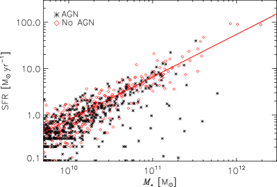
Figure 1: Star formation main sequence from our simulations. Red diamonds are for the simulation with AGN physics turned off, and black stars for the simulation including all physics. With AGN feedback included, some galaxies move off the main sequence to lower SFR. The solid red line shows the fit to the data from the simulation without AGN feedback (equation (3)).

The main aim of this paper is to gain a quantitive understanding of the relative importance of how various physical processes affect the SFR of galaxies at the present day. We start from the SFMS, which relates the SFR and stellar mass of galaxies. Observations show that star-forming, late-type galaxies (LTG) form a narrow sequence with more massive galaxies having higher SFR (e.g., Elbaz et al., 2011; Zahid et al., 2012; Renzini & Peng, 2015), while early-type galaxies (ETG) occupy a region of parameter space below this sequence (e.g., Wuyts et al., 2011; Renzini & Peng, 2015). In our simulations, AGN feedback is responsible for quenching star formation and moving galaxies off the SFMS (Taylor & Kobayashi, 2016). Fig. 1 shows our simulated SFMS both with (black stars) and without (red diamonds) AGN feedback. The solid red line in Fig. 1 shows the linear bisector fit to the data from the simulation without AGN feedback, given by

$$\log{\rm SFR}_{\rm fit}=-9.32+0.92\log M_{*},$$ (3)

where $M_{*}$ is the galaxy stellar mass (see Taylor & Kobayashi (2016) for a detailed comparison between our simulated SFMS and observational data). Using only the data from this simulation to obtain equation (3) ensures that all galaxies are star-forming and lie on the SFMS, giving a relationship with no AGN contamination.

However, as discussed in Section 1, other factors, such as the mass of gas in a galaxy, and the environment the galaxy exists in, may also affect the SFR. Feedback from star formation, supernovae, and AGN activity can remove gas from galaxies (Taylor & Kobayashi, 2015b), depending on the galaxy mass and strength of feedback. Although the feedback energy in our AGN model is calculated from the instantaneous accretion rate, the current mass of gas in the galaxy likely depends more on the BH mass, since this reflects the entire accretion history of the BH. Similarly, the total stellar mass better reflects the integrated influence of stellar feedback on the gas than the current SFR.

Therefore, in order to quantify the relative importance of these processes, we suggest the following simple model to describe SFR in all galaxies:

$${\rm SFR}=A\times M_{*}^{\alpha}\times s_{5}^{\beta}\times M_{\rm gas}^{\gamma}\times f(M_{\rm BH}),$$ (4)

where $s_{5}$ is the 3-dimensional 5^th-nearest neighbour distance, which we showed in Taylor & Kobayashi (in prep.) to be a good measure of environmental density (though numerous measures of environmental density have been proposed; see e.g., Haas et al., 2012), $M_{\rm gas}$ is the mass of gas within the galaxy, and $A$ is a constant. The function $f(M_{\rm BH})$ will be discussed in detail below.

To perform the fitting of our simulated data to this model, it is convenient to work with the logarithm of equation (4):

$$\begin{split}\log{\rm SFR}=C&+\alpha\log\left(\frac{M_{*}}{10^{10}{\,\rm M}_{\odot}}\right)+\beta\log\left(\frac{s_{5}}{10^{2}{\rm kpc}}\right)\\ &+\gamma\log\left(\frac{M_{\rm gas}}{10^{7}{\,\rm M}_{\odot}}\right)+\log f\left(\frac{M_{\rm BH}}{10^{8}{\,\rm M}_{\odot}}\right).\end{split}$$ (5)

The coefficients $C$, $\alpha$, $\beta$, and $\gamma$ are constants that will be determined by fitting (note that $\alpha$, $\beta$ and $\gamma$ are the scaling exponents for $M_{*}$, $s_{5}$, and $M_{\rm gas}$, respectively, as defined in equation (4)). $M_{*}$, $s_{5}$, $M_{\rm gas}$, and $M_{\rm BH}$ are normalised by representative quantities, such that the distribution of $\log\left(M_{*}/10^{10}{\,\rm M}_{\odot}\right)$ (and similarly for $s_{5}$, $M_{\rm gas}$, and $M_{\rm BH}$) has a modal value of about zero; this too is a fitting convenience, and affects only the value of fitted parameter $C$.

The function $f(M_{\rm BH})$ in equations (4) and (5) reflects the fact that BHs must grow sufficiently massive before their feedback energy can not be efficiently radiated away. This is illustrated in Fig. 2, which shows the residuals of SFR in the simulation with AGN compared with the SFR estimated from equation (3), as a function of BH mass. There are two clear regimes: at $M_{\rm BH}\lesssim 10^{7}{\,\rm M}_{\odot}$, the residuals are distributed around $0$, while at $M_{\rm BH}\gtrsim 10^{7}{\,\rm M}_{\odot}$ the residuals decrease with increasing $M_{\rm BH}$, and the SFR can be as much as two orders of magnitude below the SFMS.

Figure 2: Difference between measured SFR from the galaxies in the simulation with AGN feedback, and the SFR expected given the stellar masses of those galaxies and the fit to the SFMS from the simulation without AGN feedback.

This suggests the following form for $f(M_{\rm BH})$:

$$\log f_{1}(M_{\rm BH})=\begin{cases}k_{1}\log M_{\rm BH}&M_{\rm BH}<M_{\rm b},\\ k_{2}\log M_{\rm BH}+(k_{1}-k_{2})\log M_{\rm b}&M_{\rm BH}\geq M_{\rm b},\end{cases}$$ (6)

where $k_{1}$ and $k_{2}$ are constant, and $M_{\rm b}$ is a break mass at which $f(M_{\rm BH})$ turns over. In Section 4, we also test the following forms of $f(M_{\rm BH})$:

$$\log f_{2}(M_{\rm BH})=k_{1}\log M_{\rm BH},$$ (7)

$$\begin{split}\log f_{3}&(M_{\rm BH})=\frac{1}{2}(k_{1}+k_{2})\log M_{\rm BH}\\ &+\frac{1}{2}(k_{2}-k_{1})\Delta_{\rm logM}\ln\left(\cosh\left(\frac{\log M_{\rm BH}-\log M_{\rm b}}{\Delta_{\rm logM}}\right)\right).\end{split}$$ (8)

Function $f_{2}$ is the special case of $f_{1}$ in which $k_{2}=k_{1}$, i.e. there is no break. $f_{3}$ is a continuous, smooth analogue to $f_{1}$, in which the gradient varies smoothly from $k_{1}$ to $k_{2}$, with the additional parameter $\Delta_{\rm logM}$ controlling the width over which the transition occurs. Equation (8) reproduces $f_{1}$ in the limit $\Delta_{\rm logM}\rightarrow 0$. The constant of integration that would appear in equation (8) can simply be absorbed by $C$ in equation (5). We show in Fig. 3 an example of each of the three functions described above.

Figure 3: Examples of the three functions given by Models 1-3, with arbitrary example parameters $k_{1}=0.2$, $k_{2}=-2$, $\log M_{\rm b}=7$, and $\Delta_{\rm logM}=1$. Note that these values are purely illustrative; measured values are presented in Section 4.

Values of $C$, $\alpha$, $\beta$, $\gamma$, $k_{1}$, $k_{2}$, $\log M_{\rm b}$, and $\Delta_{\rm logM}$ are found using the amoeba routine (Press et al., 1992), minimising the quantity $\sum_{i}\left(\log{\rm SFR}_{i}-\log{\rm SFR}_{i,{\rm fit}}\right)^{2}$. In order to estimate uncertainties on the fitted parameters we employ a bootstrap resampling technique whereby the parameters are re-derived for a random selection of the data, with repeats, the same size as the original dataset. We do this for $5\times 10^{6}$ resamplings, in order to fully sample the parameter space of the models with the most free parameters.

4 Model Fits

Table 1: Fitted parameters of the models presented in Section 3. The parameters denote: $C$ – normalisation; $\alpha$ – coefficient of $\log M_{*}$; $\beta$ – coefficient of $\log s_{5}$, $\gamma$ – coefficient of $\log M_{\rm gas}$; $k_{1}$ – coefficient of $\log M_{\rm BH}$ (low mass); $k_{2}$ – coefficient of $\log M_{\rm BH}$ (high mass); $\log M_{\rm b}$ – break mass separating low- and high-mass BHs; $\Delta_{\rm logM}$ – width of transition from low- to high-mass BHs. Three values for each parameter are given for each model: the first is the best-fit value from the simulated data; the second is the mean and standard deviation from the full bootstrap parameter distributions; and the third is the modal value of the distributions with asymmetric errors denoting the $16^{\rm th}$ and $84^{\rm th}$ percentiles. The distribution of $\Delta_{\rm logM}$ in model 3 is bimodal, so asymmetric error bars are unavailable; this value is marked ^†.

$x$	Best Fit	$\bar{x}\pm\sigma_{x}$	Mode ${}^{+}_{-}$ distribution width
Model 1 (equation (6))
$C$	$-2.50$	$-2.59\pm 0.18$	$-2.58^{+0.18}_{-0.18}$
$\alpha$	$0.21$	$0.21\pm 0.03$	$0.21^{+0.03}_{-0.03}$
$\beta$	$-0.17$	$-0.15\pm 0.04$	$-0.16^{+0.04}_{-0.03}$
$\gamma$	$1.03$	$1.04\pm 0.05$	$1.04^{+0.05}_{-0.05}$
$k_{1}$	$0.00$	$-0.02\pm 0.03$	$-0.01^{+0.03}_{-0.04}$
$k_{2}$	$-1.11$	$-1.99\pm 3.13$	$-1.12^{+0.52}_{-0.82}$
$\log M_{\rm b}$	$7.31$	$7.79\pm 0.64$	$7.29^{+0.46}_{-0.15}$
Model 2 (equation (7))
$C$	$-2.72$	$-2.72\pm 0.15$	$-2.72^{+0.15}_{-0.14}$
$\alpha$	$0.21$	$0.21\pm 0.03$	$0.21^{+0.03}_{-0.03}$
$\beta$	$-0.12$	$-0.12\pm 0.04$	$-0.12^{+0.04}_{-0.03}$
$\gamma$	$1.05$	$1.05\pm 0.05$	$1.04^{+0.06}_{-0.05}$
$k_{1}$	$-0.05$	$-0.05\pm 0.02$	$-0.04^{+0.02}_{-0.03}$
Model 3 (equation (8))
$C$	$-3.12$	$-3.08\pm 0.19$	$-3.08^{+0.19}_{-0.18}$
$\alpha$	$0.21$	$0.22\pm 0.03$	$0.21^{+0.03}_{-0.03}$
$\beta$	$-0.16$	$-0.16\pm 0.03$	$-0.16^{+0.03}_{-0.03}$
$\gamma$	$1.05$	$1.05\pm 0.05$	$1.06^{+0.05}_{-0.05}$
$k_{1}$	$0.04$	$0.06\pm 0.05$	$0.08^{+0.03}_{-0.08}$
$k_{2}$	$-1.19$	$-1.25\pm 0.85$	$-0.82^{+0.31}_{-0.53}$
$\log M_{\rm b}$	$7.68$	$7.66\pm 0.15$	$7.58^{+0.14}_{-0.07}$
$\Delta_{\rm logM}$	$1.22$	$1.55\pm 0.76$	$2.06^{\dagger}\,\,\,\,\,\,\,\,\,\,\,$

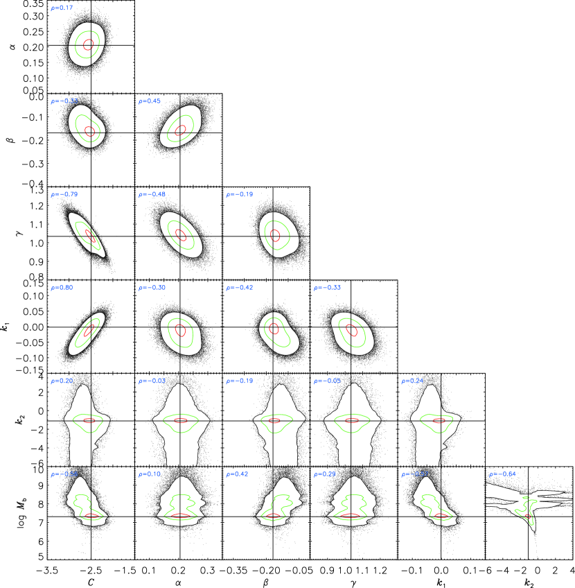
Figure 4: Parameter distributions for $f_{1}$ (equation (6)). Contours enclose 95, 68, and 16 per cent of points. The correlation coefficient, $\rho$, for each pair of parameters is shown in the upper left of each panel.

Fitting the SFR of our simulated galaxies using the method described in Section 3 to the models described in equations (5)-(8) results in the parameters given in Table 1; the full parameter distributions for $f_{1}$ are shown in Fig. 4. The uncertainties are derived from the bootstrap resampling procedure described in Section 3; the first column of Table 1 gives the best-fit parameters to the simulated data, the second gives the mean and standard deviation from the bootstrap distributions, and third shows the modal value with asymmetric errors denoting the $16^{\rm th}$ and $84^{\rm th}$ percentiles. For all three models, the values of $C$, $\alpha$, $\beta$, and $\gamma$ are consistent with one another, and are well-constrained by the data.

We find that SFR depends most strongly on the amount of gas in a galaxy, scaling linearly with $M_{\rm gas}$ ($\gamma\approx 1$). Additionally, galaxies with large stellar mass and high environmental density (low $s_{5}$) show greater SFR, with the dependence on galaxy mass being the more important (i.e., $\alpha>|\beta|$). However, with $f_{1}$ and $f_{3}$, this is tempered by the strong negative correlation between SFR and $M_{\rm BH}$ in galaxies with BHs more massive than $M_{\rm b}$ (i.e., $k_{2}$ is large and negative). Such galaxies tend to be found in the densest environments, at the centre of clusters, implying that satellite galaxies within the cluster have the highest SFRs, while field galaxies tend to have lower SFRs at a given stellar mass. This is consistent with the observational result of Koyama et al. (2013), who found that the SFR of star-forming galaxies increases with environmental density (see also Peng et al., 2010; Wijesinghe et al., 2012, who find weak or no dependence of SFR on environment for star-forming galaxies). In all models, star formation in galaxies with low-mass BHs is not strongly affected, as indicated by the value $k_{1}\sim 0$, i.e. SFR follows the SFMS for $M_{\rm BH}\lesssim M_{\rm b}$ (see Fig. 2).

The relatively large uncertainties on the values of both $k_{2}$ $\log M_{\rm b}$ in $f_{1}$ are due to their distributions, shown in Fig. 4, being highly extended, and, in the case of $\log M_{\rm b}$, nearly bimodal. In addition to the main peak around $\log M_{\rm b}\approx 7.3$, there is an extended plateau of values near $\log M_{\rm b}\sim 8$. $\log M_{\rm b}\gtrsim 8$ is found when very few of the 38 galaxies with $M_{\rm BH}>10^{7}{\,\rm M}_{\odot}$ are included in a bootstrap realisation of the data set. In such cases, none of the data constrains $M_{\rm b}$ other than being larger than the largest $M_{\rm BH}$, and so $M_{\rm b}$ can take any arbitrarily large number without affecting how well the model fits the data. This is also responsible for the very extended distribution of $k_{2}$ seen in Fig. 4.

Function $f_{3}$ produces fairly consistent values with those of $f_{1}$, favouring a slightly higher value $\log M_{\rm b}\approx 7.6$, as well as predicting a wide range of black hole masses over which AGN feedback quenches star formation with $\Delta_{\rm logM}\sim 1-2$. Similar caveats apply to $k_{2}$, $\log M_{\rm b}$, and $\Delta_{\rm logM}$ in this model as for $k_{2}$ and $\log M_{\rm b}$ in $f_{1}$. Fortunately, however, the conclusions we draw in subsequent sections do not depend on the exact values of these parameters.

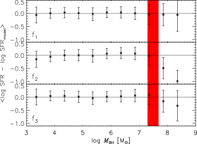
Figure 5: Residuals for the three models (assuming the best fit parameters) presented in Section 3, as a function of BH mass. The mean and standard deviation of the residuals in bins of $\log M_{\rm BH}$ with a width of 0.5 dex are shown. From top to bottom, the panels show this quantity for $f_{1}$, $f_{2}$, and $f_{3}$, respectively. The red band indicates the range of $M_{\rm b}$ from Table 1; $f_{2}$ clearly does not fit the data at $M_{\rm BH}>M_{\rm b}$.

Fig. 5 shows the residuals for each of the models $f_{1}$ to $f_{3}$ as a function of $M_{\rm BH}$. The mean and standard deviation are shown for bins with width 0.5 dex, and the red band shows the range of $M_{\rm b}$ from Table 1. At $\log M_{\rm BH}\lesssim 7$, the three models have residuals that are distributed fairly uniformly around 0, though $f_{2}$ may show a very slight increasing trend with $M_{\rm BH}$. At higher masses, $f_{2}$, which assumes that there is no break mass $M_{\rm b}$, shows a significant systematic decrease in residuals with mass that is not seen in the residuals of $f_{1}$. A similar trend is seen for the residuals of $f_{3}$, though the residuals are consistent with 0 over the full range of $M_{\rm BH}$.

5 Discussion

5.1 BH growth and AGN feedback

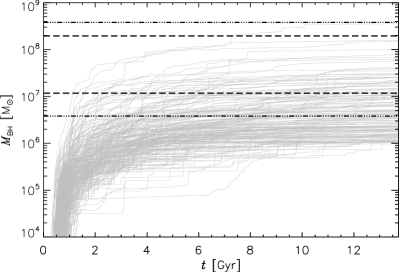
Figure 6: Mass assembly history of all BHs that grow above $10^{6}{\,\rm M}_{\odot}$ by $z=0$, as a function of the age of the Universe.

We focus now on understanding the implications of the value of $\Delta_{\rm logM}$ from $f_{3}$. It is instructive to estimate a timescale over which BHs grow by a factor $10^{\Delta_{\rm logM}}\sim 10-100$. In Fig. 6 we show the mass assembly history of all simulated BHs with final masses greater than $10^{6}{\,\rm M}_{\odot}$, and the horizontal dashed and dot-dashed lines show $M_{\rm BH}=M_{\rm b}\times 10^{\pm\frac{1}{2}\Delta_{\rm logM}}$ assuming the best-fit and modal values, respectively. It is clear that, regardless of the exact values of $M_{\rm b}$ and $\Delta_{\rm logM}$ used, the timescale for BHs to grow by a factor $10^{\Delta_{\rm logM}}$ is at least several Gyr. This should not be interpreted, however, as the timescale over which an individual BH quenches star formation in its host, since we showed in Taylor & Kobayashi (2015a) that star formation in individual galaxies can be quenched abruptly. Rather, this shows that once they grow to $\sim M_{\rm b}$, BHs have the potential to exert influence over the evolution of their galaxy.

The fact that an individual BH can quench star formation in its host much more quickly than it takes to grow by a factor $10^{\Delta_{\rm logM}}$ once it reaches $M_{\rm BH}\approx M_{\rm b}$ implies that attaining a mass $M_{\rm b}$ is a necessary but not sufficient requirement for AGN feedback to become effective. This may suggest that local properties within a galaxy can affect exactly when AGN feedback shuts off star formation, or that a ‘trigger’ for strong AGN feedback may be required once the BH is sufficiently massive, with gas-rich galaxy mergers being a likely candidate (e.g., Comerford et al., 2015; Gatti et al., 2016). The cause of strong AGN activity, such as the AGN-driven outflows described in Taylor & Kobayashi (2015b), will be investigated in detail in a future work.

5.2 Galaxy transition at $3\times 10^{10}{\,\rm M}_{\odot}$

Figure 5 shows that the model that does not include a BH break mass, $f_{2}$, does not describe our simulated data well for $M_{\rm BH}\gtrsim M_{\rm b}$. Therefore we can conclude that the influence of BHs on star formation changes once the BH grows above $M_{\rm b}$. There is an empirical relationship between $M_{\rm BH}$ and the stellar bulge mass of its host galaxy, $M_{\rm bulge}$. Converting the range of fitted values of $M_{\rm b}$ from both $f_{1}$ and $f_{3}$ ($M_{\rm b}\approx 2-5\times 10^{7}{\,\rm M}_{\odot}$) into a stellar bulge mass using the relation given in Graham & Scott (2015) gives $M_{\rm bulge}\approx 1-2\times 10^{10}{\,\rm M}_{\odot}$. At these stellar masses, galaxies typically have bulge-to-disc ($B/D$) ratios of $0.3-0.4$ (Shen et al., 2003), corresponding to bulge-to-total ($B/T$) ratios of $0.23-0.29$ (note that ETGs can have much larger $B/T\sim 0.7$; see, e.g., Morselli et al., 2017). For such values of $B/T$, $M_{\rm b}$ corresponds to a galaxy mass that is consistent with the galaxy mass of $M_{*}=3\times 10^{10}{\,\rm M}_{\odot}$ found by Kauffmann et al. (2003) to separate ETGs and LTGs.

This consistency between our simulations and observational data implies that feedback from super-massive BHs may be responsible for the transition from LTGs to ETGs at $M_{*}=3\times 10^{10}{\,\rm M}_{\odot}$. Such a result is in broad agreement with other studies; Keller et al. (2016) find that even very strong supernova feedback in the form of superbubbles is inefficient in galaxies $M_{*}\gtrsim 4\times 10^{10}{\,\rm M}_{\odot}$, arguing that AGN feedback must dominate in more massive galaxies. Similarly, Bower et al. (2017) find that BH accretion is suppressed by supernova feedback in galaxies less massive than $3\times 10^{10}{\,\rm M}_{\odot}$, with AGN feedback becoming important once supernova feedback can no longer remove gas from the galaxy potential. In this paper, we have not investigated why strong AGN feedback is triggered in massive galaxies, finding only that it is triggered once a BH grows to $M_{\rm b}\approx 2-5\times 10^{7}{\,\rm M}_{\odot}$. The reason for the triggering will be investigated in detail in a future work.

5.3 Connection to the Kennicutt-Schmidt Law

The Kennicutt-Schmidt (KS) law is an empirical relation between SFR surface density $\Sigma_{\rm SFR}$, and gas surface density, $\Sigma_{\rm gas}$ (Schmidt, 1959; Kennicutt, 1989; Kennicutt & Evans, 2012). With $\gamma\approx 1$ (the exponent of $M_{\rm gas}$ in our model), dividing equation (4) by galaxy area gives $\Sigma_{\rm SFR}\sim\Sigma_{\rm gas}$. Observations typically find a super-linear relation when all gas is considered (e.g., Kennicutt, 1989, 1998), as we have done, while a linear or sub-linear relation tends to be found when only dense gas is considered (e.g., Bigiel et al., 2008; Shetty et al., 2013, 2014, but see also Liu et al. 2011; Momose et al. 2013). Shetty et al. (2014) analysed disk galaxies from the STING survey and concluded that galactic properties other than $\Sigma_{\rm gas}$ affect $\Sigma_{\rm SFR}$; such properties were included in our model, which may explain the difference between our linear relationship and observations (though there is significant scatter in the KS relation; see e.g. Krumholz et al., 2012; Federrath, 2013; Salim et al., 2015). We note for completeness that if we only consider SFR and $M_{\rm gas}$, we obtain a slope $1.54\pm 0.03$, in much better agreement with the observed super-linear relation of Kennicutt (1989, 1998).

5.4 The star formation main sequence

Regardless of the form of $f(M_{\rm BH})$ used, Table 1 shows that $\alpha=0.21$, i.e. $\log{\rm SFR}\sim 0.21\log M_{*}$. This is in contrast to observational estimates, which find a present-day slope around 0.75 – 1 (e.g., Elbaz et al., 2007, 2011; Zahid et al., 2012; Renzini & Peng, 2015). This is due to the correlations between stellar mass and other physical properties that are not accounted for in the standard SFMS, but are in this model, as was the case for the KS relation above. Our results suggest that stellar mass is not as important in determining galactic SFR as implied by the standard SFMS, and that there is an environmental dependence as well as strong gas mass dependence on the SFR of star-forming galaxies.

6 Comparison of our new SFR Model to observational data

We test our star formation models by comparing to observations. Ideally, we would wish to repeat the analysis of Section 4 on observational data to critically appraise our star formation model and our simulations. However, there are no overlapping surveys that can provide all of SFR, $M_{*}$, $s_{5}$, $M_{\rm gas}$, and $M_{\rm BH}$ for a large number of galaxies. By searching the literature and various current observational databases, we were able to find a sample of galaxies for which all the required measurements of SFR, $M_{*}$, $s_{5}$, and $M_{\rm gas}$ were available (except $M_{\rm BH}$). We use this set of galaxies to compare their measured SFR with that estimated from our model.

The Galaxy And Mass Assembly survey (GAMA, Driver et al., 2011) is an optical survey using the Anglo-Australian Telescope and AAOmega spectrograph (Sharp et al., 2006). It is $>$98 per cent complete to a depth of $r<19.4$ or $19.8$. The survey is spread over three $12^{\circ}$ by $4^{\circ}$ equatorial regions. Environmental density data are only available for 16,062 galaxies in the region centred at 15h right ascension. In this paper, we use aperture-corrected $M_{*}$ (Taylor et al., 2011), SFR (Gunawardhana et al., 2011), and $s_{5}$ (Brough et al., 2013) data for these galaxies.

For the gas masses, we use data from the Arecibo Legacy Fast ALFA survey (ALFALFA, Giovanelli et al., 2005). ALFALFA is a wide-field survey using the Arecibo radio telescope to map the 21 cm line of atomic hydrogen. Corresponding HI masses, $M_{\rm HI}$ are derived in Haynes et al. (2011); to convert this to total gas mass, we make the simplistic assumptions that 1) $M_{\rm HI}$ is equal to the total mass of hydrogen in the ISM, and 2) the ISM has primordial composition, so that $M_{\rm gas}=M_{\rm HI}/0.75$. We associate HI detections from ALFALFA with an optical counterpart in GAMA if they are separated by less than $0\aas@@fstack{\circ}01$ in RA and Dec. Matching the catalogues in this way gives 14 galaxies with measured $M_{*}$, SFR, $s_{5}$, and $M_{\rm gas}$.

Figure 7: Comparison of measured SFR (SFR_obs) and predicted SFR (SFR_model) from our model, using the best-fit parameters of Model 1 (equations (5) and (6), and Table 1), for galaxies selected from the GAMA and ALFALFA surveys. The solid line denotes SFR${}_{\rm model}={\rm SFR}_{\rm obs}$. Filled circles with error bars show the results of equation (9), while diamond and star symbols are for if $M_{\rm gas}$ or $M_{\rm gas}$ and $s_{5}$ are excluded, respectively. Error bars on SFR_model include both errors on observed quantities and uncertainties in the model parameter values; no error information was available for SFR_obs.

We estimate the SFR of these galaxies assuming the best-fit parameters of Model 1, neglecting any contribution from BHs, i.e.,

$$\begin{split}\log&\left({\rm SFR}_{\rm model}\right)=-2.50+0.21\log\left(\frac{M_{*}}{10^{10}{\,\rm M}_{\odot}}\right)\\ &-0.17\log\left(\frac{s_{5}}{100\,{\rm kpc}}\right)+1.03\log\left(\frac{M_{\rm HI}}{0.75\times 10^{7}{\,\rm M}_{\odot}}\right).\end{split}$$ (9)

The most massive of these 14 galaxies has $M_{*}=1.7\times 10^{10}{\,\rm M}_{\odot}$, and so we expect to be in the parameter space where BH feedback does not play a crucial role for the SFR, i.e. $\log f\sim k_{1}M_{\rm BH}\sim 0$. Higher-mass galaxies with $M_{*}$, $s_{5}$, $M_{\rm gas}$, and simultaneous $M_{\rm BH}$ measurements are needed in the future to test our predicted dependence of the SFR on BH mass.

In Fig. 7 we show the measured SFR (SFR_obs) and the SFR predicted by our model (SFR_model) for these galaxies (filled circles with error bars). The agreement between the observed SFR and those predicted by our model is extremely encouraging, considering the assumptions used to calculate $M_{\rm gas}$ and the fact that $s_{5}$ from the GAMA catalogue is projected, whereas we used the 3-D $s_{5}$ in deriving our model parameters. Also shown in Fig. 7 are the predicted SFRs if $M_{\rm gas}$ or $M_{\rm gas}$ and $s_{5}$ are excluded (diamond and star symbols, respectively). In both cases, the model SFR is significantly less than is observed, and shows little evidence of correlation with the observed values. This reinforces the fact that $M_{\rm gas}$ is the most important quantity in determining SFR. The inclusion of $s_{5}$ alters the predicted SFR very little, but may be more important in more extreme environments such as galaxy groups and clusters (e.g., Schaefer et al., 2017).

In the coming decade, vast radio surveys such as the Square Kilometre Array (SKA) and its precursors will provide HI masses for tens of thousands of galaxies, allowing for a more rigorous test of our model. However, black hole masses are more difficult to measure, and are available for only a relatively small number of galaxies in the local Universe. Directly validating our full model including the effects of BHs will be a challenging, but important task for the near future.

7 Conclusions

We have analysed data from a cosmological hydrodynamical simulation that includes a detailed prescription for star formation and stellar feedback, as well as BH formation and AGN feedback. Our aim was to understand better the relative importance of factors that affect SFR of galaxies. We suggested that SFR could be influenced by the mass of the host galaxy, its environmental density, its gas content, and the mass of its BH. We proposed a relatively simple form for the relation between SFR and host galaxy properties (equation (5)), with which we were able to make quantitative comparisons.

We find that once a BH has grown sufficiently massive ($\sim 2-5\times 10^{7}{\,\rm M}_{\odot}$), it can be triggered to shut off star formation through AGN feedback; the details of such triggering will be investigated in future work. Such a BH mass corresponds, via the Maggorian relation (Graham & Scott, 2015), to a galaxy bulge mass of $\sim 1-2\times 10^{10}{\,\rm M}_{\odot}$, which is consistent with the observed galaxy mass above which ETGs make up the dominant fraction of the galaxy population ($\sim 3\times 10^{10}{\,\rm M}_{\odot}$, Kauffmann et al., 2003). It is important to note that these masses are emergent in our simulations; none of the input parameters of the baryon physics is chosen to yield such a transition mass, but are constrained by other observations.

The SFR depends strongly on the amount of gas in a galaxy, scaling approximately linearly with gas mass, while the dependence on stellar mass is weaker than predicted from the standard SFMS since we take into account the correlations between SFR and the additional physical quantities $M_{\rm gas}$, $s_{5}$, and $M_{\rm BH}$ by fitting all simultaneously. Our simulation cannot resolve the cold molecular gas that would form stars, and in this analysis we have treated all gas equally, regardless of temperature or density. In light of this, it will be useful in future works to analyse galaxies simulated with sufficient resolution to distinguish between gas phases.

We find that star-forming galaxies in high density regions have larger SFR than star-forming galaxies in the field at given mass, in agreement with observations (e.g., Koyama et al., 2013). This would most likely evolve with redshift, with massive galaxies showing the highest SFR in the past. The existence and strength of any such evolution will be investigated in a future work. Furthermore, the size of our simulation box limits the size of our most massive simulated cluster, and it would be informative to investigate if the trends seen here hold for more extreme environments.

We use observational data from the GAMA and ALFALFA surveys to compare the SFR observed with that predicted by our new model (see Fig. 7). There is excellent agreement between these two quantities, lending credence to the model we have presented. The sample is limited by the available observations, but will increase to tens of thousands in the era of the SKA. Further validation of our model will only be possible with a catalogue of BH masses for large numbers of galaxies.

References

- Agarwal et al. (2012) Agarwal B., Khochfar S., Johnson J. L., Neistein E., Dalla Vecchia C., Livio M., 2012, MNRAS, 425, 2854
- Baldry et al. (2006) Baldry I. K., Balogh M. L., Bower R. G., Glazebrook K., Nichol R. C., Bamford S. P., Budavari T., 2006, MNRAS, 373, 469
- Barnes & Hernquist (1996) Barnes J. E., Hernquist L., 1996, ApJ, 471, 115
- Becerra et al. (2015) Becerra F., Greif T. H., Springel V., Hernquist L. E., 2015, MNRAS, 446, 2380
- Bicknell et al. (2000) Bicknell G. V., Sutherland R. S., van Breugel W. J. M., Dopita M. A., Dey A., Miley G. K., 2000, ApJ, 540, 678
- Bieri et al. (2016) Bieri R., Dubois Y., Silk J., Mamon G. A., Gaibler V., 2016, MNRAS, 455, 4166
- Bigiel et al. (2008) Bigiel F., Leroy A., Walter F., Brinks E., de Blok W. J. G., Madore B., Thornley M. D., 2008, AJ, 136, 2846
- Birnboim et al. (2016) Birnboim Y., Padnos D., Zinger E., 2016, ApJ, 832, L4
- Boselli & Gavazzi (2006) Boselli A., Gavazzi G., 2006, PASP, 118, 517
- Bower et al. (2017) Bower R. G., Schaye J., Frenk C. S., Theuns T., Schaller M., Crain R. A., McAlpine S., 2017, MNRAS, 465, 32
- Bromm et al. (2002) Bromm V., Coppi P. S., Larson R. B., 2002, ApJ, 564, 23
- Bromm & Loeb (2003) Bromm V., Loeb A., 2003, ApJ, 596, 34
- Brough et al. (2013) Brough S. et al., 2013, MNRAS, 435, 2903
- Bundy et al. (2006) Bundy K. et al., 2006, ApJ, 651, 120
- Cen (2014) Cen R., 2014, ApJ, 789, L21
- Chabrier (2003) Chabrier G., 2003, PASP, 115, 763
- Cicone et al. (2012) Cicone C., Feruglio C., Maiolino R., Fiore F., Piconcelli E., Menci N., Aussel H., Sturm E., 2012, A&A, 543, A99
- Combes et al. (1990) Combes F., Debbasch F., Friedli D., Pfenniger D., 1990, A&A, 233, 82
- Comerford et al. (2015) Comerford J. M., Pooley D., Barrows R. S., Greene J. E., Zakamska N. L., Madejski G. M., Cooper M. C., 2015, ApJ, 806, 219
- Cowie et al. (1996) Cowie L. L., Songaila A., Hu E. M., Cohen J. G., 1996, AJ, 112, 839
- Darg et al. (2010) Darg D. W. et al., 2010, MNRAS, 401, 1552
- Dekel et al. (2009) Dekel A., Sari R., Ceverino D., 2009, ApJ, 703, 785
- Dressler & Gunn (1983) Dressler A., Gunn J. E., 1983, ApJ, 270, 7
- Driver et al. (2011) Driver S. P. et al., 2011, MNRAS, 413, 971
- Elbaz et al. (2007) Elbaz D. et al., 2007, A&A, 468, 33
- Elbaz et al. (2011) Elbaz D. et al., 2011, A&A, 533, A119
- Elmegreen & Scalo (2004) Elmegreen B. G., Scalo J., 2004, ARA&A, 42, 211
- Federrath (2013) Federrath C., 2013, MNRAS, 436, 3167
- Federrath & Klessen (2012) Federrath C., Klessen R. S., 2012, ApJ, 761, 156
- Feldmann et al. (2016) Feldmann R., Quataert E., Hopkins P. F., Faucher-Giguère C.-A., Kereš D., 2016, ArXiv e-prints:1610.02411
- Feruglio et al. (2010) Feruglio C., Maiolino R., Piconcelli E., Menci N., Aussel H., Lamastra A., Fiore F., 2010, A&A, 518, L155
- Gatti et al. (2016) Gatti M., Shankar F., Bouillot V., Menci N., Lamastra A., Hirschmann M., Fiore F., 2016, MNRAS, 456, 1073
- Gavazzi et al. (1995) Gavazzi G., Randone I., Branchini E., 1995, ApJ, 438, 590
- Giovanelli et al. (2005) Giovanelli R. et al., 2005, AJ, 130, 2598
- Graham & Scott (2015) Graham A. W., Scott N., 2015, ApJ, 798, 54
- Gunawardhana et al. (2011) Gunawardhana M. L. P. et al., 2011, MNRAS, 415, 1647
- Gunn & Gott (1972) Gunn J. E., Gott III J. R., 1972, ApJ, 176, 1
- Haardt & Madau (1996) Haardt F., Madau P., 1996, ApJ, 461, 20
- Haas et al. (2012) Haas M. R., Schaye J., Jeeson-Daniel A., 2012, MNRAS, 419, 2133
- Haynes et al. (2011) Haynes M. P. et al., 2011, AJ, 142, 170
- Heckman et al. (2000) Heckman T. M., Lehnert M. D., Strickland D. K., Armus L., 2000, ApJS, 129, 493
- Hinshaw et al. (2013) Hinshaw G. et al., 2013, ApJS, 208, 19
- Hopkins et al. (2008) Hopkins P. F., Hernquist L., Cox T. J., Kereš D., 2008, ApJS, 175, 356
- Hopkins et al. (2014) Hopkins P. F., Kereš D., Oñorbe J., Faucher-Giguère C.-A., Quataert E., Murray N., Bullock J. S., 2014, MNRAS, 445, 581
- Hosokawa et al. (2016) Hosokawa T., Hirano S., Kuiper R., Yorke H. W., Omukai K., Yoshida N., 2016, ApJ, 824, 119
- Juneau et al. (2005) Juneau S. et al., 2005, ApJ, 619, L135
- Kauffmann et al. (2003) Kauffmann G. et al., 2003, MNRAS, 341, 54
- Kaviraj (2014) Kaviraj S., 2014, MNRAS, 437, L41
- Keller et al. (2016) Keller B. W., Wadsley J., Couchman H. M. P., 2016, MNRAS, 463, 1431
- Kennicutt & Evans (2012) Kennicutt R. C., Evans N. J., 2012, ARA&A, 50, 531
- Kennicutt (1989) Kennicutt Jr. R. C., 1989, ApJ, 344, 685
- Kennicutt (1998) Kennicutt Jr. R. C., 1998, ApJ, 498, 541
- Kobayashi (2004) Kobayashi C., 2004, MNRAS, 347, 740
- Kobayashi et al. (2011) Kobayashi C., Karakas A. I., Umeda H., 2011, MNRAS, 414, 3231
- Kobayashi & Nakasato (2011) Kobayashi C., Nakasato N., 2011, ApJ, 729, 16
- Kobayashi & Nomoto (2009) Kobayashi C., Nomoto K., 2009, ApJ, 707, 1466
- Kobayashi et al. (2007) Kobayashi C., Springel V., White S. D. M., 2007, MNRAS, 376, 1465
- Kobayashi et al. (2006) Kobayashi C., Umeda H., Nomoto K., Tominaga N., Ohkubo T., 2006, ApJ, 653, 1145
- Koushiappas et al. (2004) Koushiappas S. M., Bullock J. S., Dekel A., 2004, MNRAS, 354, 292
- Koyama et al. (2013) Koyama Y. et al., 2013, MNRAS, 434, 423
- Kraft et al. (2009) Kraft R. P. et al., 2009, ApJ, 698, 2036
- Kroupa (2008) Kroupa P., 2008, in Knapen J. H., Mahoney T. J., Vazdekis A., eds, Astronomical Society of the Pacific Conference Series Vol. 390, Pathways Through an Eclectic Universe. p. 3
- Kroupa et al. (2013) Kroupa P., Weidner C., Pflamm-Altenburg J., Thies I., Dabringhausen J., Marks M., Maschberger T., 2013, The Stellar and Sub-Stellar Initial Mass Function of Simple and Composite Populations. Springer, Dordrecht, p. 115
- Krumholz et al. (2012) Krumholz M. R., Dekel A., McKee C. F., 2012, ApJ, 745, 69
- Liu et al. (2011) Liu G., Koda J., Calzetti D., Fukuhara M., Momose R., 2011, ApJ, 735, 63
- Lynds (1967) Lynds C. R., 1967, ApJ, 147, 396
- Mac Low & Klessen (2004) Mac Low M.-M., Klessen R. S., 2004, Reviews of Modern Physics, 76, 125
- Madau & Rees (2001) Madau P., Rees M. J., 2001, ApJ, 551, L27
- McKee & Ostriker (2007) McKee C. F., Ostriker E. C., 2007, ARA&A, 45, 565
- Mihos & Hernquist (1994) Mihos J. C., Hernquist L., 1994, ApJ, 431, L9
- Mihos & Hernquist (1996) Mihos J. C., Hernquist L., 1996, ApJ, 464, 641
- Momose et al. (2013) Momose R. et al., 2013, ApJ, 772, L13
- Moore et al. (1996) Moore B., Katz N., Lake G., Dressler A., Oemler A., 1996, Nat, 379, 613
- Morselli et al. (2017) Morselli L., Popesso P., Erfanianfar G., Concas A., 2017, A&A, 597, A97
- Ohyama et al. (2002) Ohyama Y. et al., 2002, PASJ, 54, 891
- Padoan et al. (2014) Padoan P., Federrath C., Chabrier G., Evans II N. J., Johnstone D., Jørgensen J. K., McKee C. F., Nordlund Å., 2014, Protostars and Planets VI, pp 77–100
- Peng et al. (2010) Peng Y.-j. et al., 2010, ApJ, 721, 193
- Pettini et al. (2000) Pettini M., Steidel C. C., Adelberger K. L., Dickinson M., Giavalisco M., 2000, ApJ, 528, 96
- Press et al. (1992) Press W. H., Teukolsky S. A., Vetterling W. T., Flannery B. P., 1992, Numerical Recipes in C (2Nd Ed.): The Art of Scientific Computing. Cambridge University Press, New York, NY, USA
- Regan et al. (2016) Regan J. A., Johansson P. H., Wise J. H., 2016, MNRAS, 459, 3377
- Renzini & Peng (2015) Renzini A., Peng Y.-j., 2015, ApJ, 801, L29
- Salim et al. (2015) Salim D. M., Federrath C., Kewley L. J., 2015, ApJ, 806, L36
- Salpeter (1955) Salpeter E. E., 1955, ApJ, 121, 161
- Schaefer et al. (2017) Schaefer A. L. et al., 2017, MNRAS, 464, 121
- Schmidt (1959) Schmidt M., 1959, ApJ, 129, 243
- Schneider et al. (2002) Schneider R., Ferrara A., Natarajan P., Omukai K., 2002, ApJ, 571, 30
- Semenov et al. (2016) Semenov V. A., Kravtsov A. V., Gnedin N. Y., 2016, ApJ, 826, 200
- Shabala et al. (2015) Shabala S., Crockett R. M., Kaviraj S., 2015, Highlights of Astronomy, 16, 133
- Sharp et al. (2006) Sharp R. et al., 2006, in Society of Photo-Optical Instrumentation Engineers (SPIE) Conference Series. p. 62690G
- Shen et al. (2003) Shen S., Mo H. J., White S. D. M., Blanton M. R., Kauffmann G., Voges W., Brinkmann J., Csabai I., 2003, MNRAS, 343, 978
- Shetty et al. (2013) Shetty R., Kelly B. C., Bigiel F., 2013, MNRAS, 430, 288
- Shetty et al. (2014) Shetty R., Kelly B. C., Rahman N., Bigiel F., Bolatto A. D., Clark P. C., Klessen R. S., Konstandin L. K., 2014, MNRAS, 437, L61
- Silk (2013) Silk J., 2013, ApJ, 772, 112
- Springel (2005) Springel V., 2005, MNRAS, 364, 1105
- Stringer et al. (2009) Stringer M. J., Benson A. J., Bundy K., Ellis R. S., Quetin E. L., 2009, MNRAS, 393, 1127
- Sutherland & Dopita (1993) Sutherland R. S., Dopita M. A., 1993, ApJS, 88, 253
- Taylor et al. (2011) Taylor E. N. et al., 2011, MNRAS, 418, 1587
- Taylor & Kobayashi (2014) Taylor P., Kobayashi C., 2014, MNRAS, 442, 2751
- Taylor & Kobayashi (2015a) Taylor P., Kobayashi C., 2015a, MNRAS, 448, 1835
- Taylor & Kobayashi (2015b) Taylor P., Kobayashi C., 2015b, MNRAS, 452, L59
- Taylor & Kobayashi (2016) Taylor P., Kobayashi C., 2016, MNRAS, 463, 2465
- Teng et al. (2014) Teng S. H. et al., 2014, ApJ, 785, 19
- Tombesi et al. (2013) Tombesi F., Cappi M., Reeves J. N., Nemmen R. S., Braito V., Gaspari M., Reynolds C. S., 2013, MNRAS, 430, 1102
- Toomre & Toomre (1972) Toomre A., Toomre J., 1972, ApJ, 178, 623
- Wijesinghe et al. (2012) Wijesinghe D. B. et al., 2012, MNRAS, 423, 3679
- Wuyts et al. (2011) Wuyts S. et al., 2011, ApJ, 742, 96
- Zahid et al. (2012) Zahid H. J., Dima G. I., Kewley L. J., Erb D. K., Davé R., 2012, ApJ, 757, 54
- Zubovas et al. (2013) Zubovas K., Nayakshin S., King A., Wilkinson M., 2013, MNRAS, 433, 3079