Solving Constrained Horn Clauses Using
Dependence-Disjoint Expansions

Abstract

Recursion-free Constrained Horn Clauses (CHCs) are logic-programming problems that can model safety properties of programs with bounded iteration and recursion. In addition, many CHC solvers reduce recursive systems to a series of recursion-free CHC systems that can each be solved efficiently.

In this paper, we define a novel class of recursion-free systems, named Clause-Dependence Disjoint (CDD), that generalizes classes defined in previous work. The advantage of this class is that many CDD systems are smaller than systems which express the same constraints but are part of a different class. This advantage in size allows CDD systems to be solved more efficiently than their counterparts in other classes. We implemented a CHC solver named Shara. Shara solves arbitrary CHC systems by reducing the input to a series of CDD systems. Our evaluation indicates that Shara outperforms state-of-the-art implementations in many practical cases.

1 Introduction

Many critical problems in program verification can be reduced to solving systems of Constrained Horn Clauses (CHCs), a class of logic-programming problems [5, 6, 21, 22]. A CHC is a logical implication with the following form:

$$R_{\_}1(\vec{v_{\_}1})\leftarrow R_{\_}2(\vec{v_{\_}2})\land R_{\_}3(\vec{v_{\_}3})\land...\land\varphi(\vec{v_{\_}0},\vec{v_{\_}1},\vec{v_{\_}2},\vec{v_{\_}3},...)$$

Here, the left side of the implication, called the head, contains an uninterpreted relational predicate applied to a vector of variables. The right side has any number of such predicates conjoined together with a constraint ($\varphi$). The constraint is a logical formula in a background theory and may use variables named by the predicates. A CHC system is a set of CHCs. The goal of the CHC solving problem is to find suitable interpretations for each predicate such that each CHC is logically consistent in isolation.

In this work we focus on the subclass of CHC systems which are known as recursion-free. In a recursion-free CHC system, no derivation of a predicate will invoke that predicate. Less formally, a recursion-free CHC system is one where following implication arrows through the system will never reach the same clause twice. Recursion-free CHC systems are an important subclass for two reasons. First, recursion-free systems can be used to model safety properties for hierarchical programs [15, 16] (programs with only bounded iteration and recursion). Second and most importantly, a well-known approach for solving a general CHC system reduces the input problem to solving a sequence of recursion-free systems. Such approaches attempt to synthesize a solution for the original system from the solutions of recursion-free systems [5]. The performance of such solvers relies heavily on the performance of solving recursion-free CHC systems.

Typically, even recursion-free CHC systems are not solved directly. Instead, they are reduced to a more specific subclass of recursion-free CHC system. These classes include those of body-disjoint (or derivation tree) systems [11, 5, 19, 21, 22] and of linear systems [2]. We will discuss these classes in § 2 and § 6. Such classes can be solved by issuing interpolation queries to find suitable definitions for the uninterpreted predicates.

In general, solving a recursion-free CHC system for propositional logic and the theory of linear integer arithmetic is co-NEXPTIME-complete [22]. In contrast, solving a linear system or body-disjoint system with the same logic and theories is in co-NP [22]. We refer to such classes that are solvable in co-NP time as directly solvable. Because solving an arbitrary recursion-free system is harder than solving a directly solvable system, solvers which reduce to directly solvable systems are highly reliant on the size of the reductions.

The first contribution of this paper is the introduction of a novel class of directly solvable systems that we refer to as Clause-Dependence Disjoint (CDD). The formal definition of CDD is given at  Defn. 5. CDD is a strict superset of the union of previously introduced classes of directly solvable systems. The key characteristic of this class is that when an arbitrary recursion-free system is reduced to a CDD system and to a system from a different directly solvable class, the CDD system is frequently the smaller of the two. Therefore, solving recursion-free systems by reducing them to CDD form is often less computationally expensive than reducing them to a system in a different class.

The second contribution of this paper is a solver for CHC systems, named Shara. Given a recursion-free system $S$, Shara reduces the problem of solving $S$ to solving a CDD system $S^{\prime}$. In the worst case, it is possible that the size of $S^{\prime}$ may be exponential in the size of $S$. However, empirically we have found that the size of $S^{\prime}$ is usually close enough to the size of $S$ that Shara frequently outperforms Duality, one of the best known CHC solvers. The procedure implemented in Shara is a generalization of existing techniques that synthesize compact verification conditions for hierarchical programs [7, 15]. Given a general (possibly recursive) CHC system, Shara solves a sequence of recursion-free systems. Each subsystem is a bounded unwinding of the original system. Shara attempts to combine the solutions of these recursion-free systems to synthesize a solution to the original problem, as has been proposed in previous work [22].

We implemented Shara within the Duality CHC solver [5], which is implemented within the Z3 automatic theorem prover [20]. We evaluated the effectiveness of Shara on standard benchmarks drawn from SVCOMP15 [8]. The results indicate that Shara outperforms modern solvers many cases. Futhermore, the results indicate that combining the strengths of Shara with that of other existing approaches (as discussed in § 5) is a promising direction for the future of CHC solving.

The rest of this paper is organized as follows. § 2 illustrates the operation of Shara on a recursion-free CHC system. § 3 reviews technical work on which Shara is based. § 4 describes Shara in technical detail. § 5 gives the results of our empirical evaluation of Shara. § 6 compares Shara to related work.

2 Overview

In § 2.1, we describe a recursion-free CHC system, $\mbox{{S}}_{\mbox{{DA}}}$ (Figure 2), that models the safety of the program dblAbs (Figure 2). In § 2.2, we show that $\mbox{{S}}_{\mbox{{DA}}}$ is a CDD system and how Shara can solve it by encoding it into binary interpolants. In § 2.3, we illustrate that $\mbox{{S}}_{\mbox{{DA}}}$ is not in directly solvable classes introduced in previous work.

2.1 Verifying dblAbs: an example hierarchical program

[2] [.3]

Figure 1: dblAbs: an example hierarchical program.

⬇

1def dbl(int x)

2 return 2 * x

3def main(n)

4 abs = 0

5 if (n >= 0)

6 abs = n

7 else

8 abs = $-$n

9 res = dbl(abs)

10 assert(res >= 0)

Figure 2: A CHC system that models the safety condition of dblAbs, named $\mbox{{S}}_{\mbox{{DA}}}$.

[.66]

$$\mbox{{dbl}}(\mbox{{x}},\mbox{{d}}) \leftarrow\mbox{{d}}=2*\mbox{{x}}$$ (1)

$$\mbox{{L}}_{\_}4(\mbox{{n}},\mbox{{abs}}) \leftarrow\mbox{{abs}}=0$$ (2)

$$\mbox{{L}}_{\_}6(\mbox{{n}},\mbox{{abs}}) \leftarrow\mbox{{L}}_{\_}4(\mbox{{n}},\mbox{{abs}})\land\mbox{{n}}\geq 0$$ (3)

$$\mbox{{L}}_{\_}8(\mbox{{n}},\mbox{{abs}}) \leftarrow\mbox{{L}}_{\_}4(\mbox{{n}},\mbox{{abs}})\land\mbox{{n}}<0$$ (4)

$$\mbox{{L}}_{\_}9(\mbox{{n}},\mbox{{abs'}}) \leftarrow\mbox{{L}}_{\_}6(\mbox{{n}},\mbox{{abs}})\land\mbox{{abs'}}=\mbox{{n}}$$ (5)

$$\mbox{{L}}_{\_}9(\mbox{{n}},\mbox{{abs'}}) \leftarrow\mbox{{L}}_{\_}8(\mbox{{n}},\mbox{{abs}})\land\mbox{{abs'}}=-\mbox{{n}}$$ (6)

$$\mbox{{main}}(\mbox{{n}},\mbox{{res}}) \leftarrow\mbox{{L}}_{\_}9(\mbox{{n}},\mbox{{abs'}})\land\mbox{{dbl}}(\mbox{{x}},\mbox{{d}})\land\mbox{{abs'}}=\mbox{{x}}\land\mbox{{res}}=\mbox{{d}}$$ (7)

$$False \leftarrow\mbox{{main}}(\mbox{{n}},\mbox{{res}})\land\mbox{{res}}<0$$ (8)

dblAbs is a procedure that doubles the absolute value of its input and stores the result in res. The program also asserts that res is greater than or equal to $0$ before exiting. Verifying this assertion reduces to solving a recursion-free CHC system over a set of uninterpreted predicates that represent the control locations in dblAbs. In particular, one such system, $\mbox{{S}}_{\mbox{{DA}}}$, is shown in Figure 2. While $\mbox{{S}}_{\mbox{{DA}}}$ has been presented as the result of a translation from dblAbs, Shara is purely a solver for CHC systems: it does not require access to the concrete representation of a program, or for a given CHC system to be the result of translation from a program at all.

2.2 $\mbox{{S}}_{\mbox{{DA}}}$ as a Clause-Dependence Disjoint System

The recursion-free CHC system $\mbox{{S}}_{\mbox{{DA}}}$ is a Clause-Dependence Disjoint (CDD) system. A CHC system can be classified as CDD when each clause satisfies the following rules: (1) no two predicates in the body of the same clause share any transitive dependencies on other predicates and (2) no clause has more than one occurrence of a given predicate in the body. As an example, clause $(7)$ is dependence disjoint. Two predicates $\mbox{{L}}_{\_}9$ and dbl are in its body. The transitive dependency of $\mbox{{L}}_{\_}9$ is the set $\{\mbox{{L}}_{\_}4,\mbox{{L}}_{\_}6,\mbox{{L}}_{\_}8\}$ while the transitive dependency of dbl is the empty set. Therefore, their transitive dependencies are disjoint: $\{\mbox{{L}}_{\_}4,\mbox{{L}}_{\_}6,\mbox{{L}}_{\_}8\}\cap\varnothing=\varnothing$. All other clauses in $\mbox{{S}}_{\mbox{{DA}}}$ have at most one uninterpreted predicate in the body, so they are trivially disjoint dependent. Therefore $\mbox{{S}}_{\mbox{{DA}}}$ is a CDD system. The formal definition of CDD and its key properties are given in § 4.1. The formal definition of transitive dependency is given in § 3.1.

Shara solves CDD systems directly by issuing a binary interpolation query for each uninterpreted predicate in topological order. Each interpretation of a predicate $P$ can be computed by interpolating (1) the pre-formula, constructed from clauses where $P$ is the head, and (2) the post-formula, constructed from all clauses where the head transitively depends on $P$.

For example, consider $\mbox{{L}}_{\_}9$. By the time Shara attempts to synthesize an interpretation for $\mbox{{L}}_{\_}9$ it will have solutions for $\mbox{{L}}_{\_}4$, $\mbox{{L}}_{\_}6$, $\mbox{{L}}_{\_}8$. Possible interpretations of these predicates are shown in Figure 4. The pre-formula is constructed from the bodies of clauses where $\mbox{{L}}_{\_}9$ is the head. Each relational predicate, $P$, is replaced by a corresponding boolean indicator variable, $\mbox{{b}}_{\_}P$. Each boolean indicator variable implies the solution for its predicate, encoded as the disjunction of the negation of the boolean indicator variable and the solution. In particular, the pre-formula for $\mbox{{L}}_{\_}9$ is constructed from clauses (5) and (6):

$$((\mbox{{b}}_{\_}{\mbox{{L}}_{\_}6}\land\mbox{{abs'}}=\mbox{{n}})\lor(\mbox{{b}}_{\_}{\mbox{{L}}_{\_}8}\land\mbox{{abs'}}=-\mbox{{n}}))\land(\neg\mbox{{b}}_{\_}{\mbox{{L}}_{\_}6}\lor\mbox{{n}}\geq 0)\land(\neg\mbox{{b}}_{\_}{\mbox{{L}}_{\_}8}\lor\mbox{{n}}<0)$$ (9)

The post-formula is constructed from clauses that transitively depend on $\mbox{{L}}_{\_}9$. Again, we replace relational predicates by corresponding boolean indicators. However, we omit the boolean indicator for $\mbox{{L}}_{\_}9$. The post-formula is composed from clauses (1), (7), and (8):

$$(\neg\mbox{{b}}_{\_}{\mbox{{dbl}}}\lor\mbox{{d}}=2*\mbox{{x}})\land(\neg\mbox{{b}}_{\_}{\mbox{{main}}}\lor(\mbox{{b}}_{\_}{\mbox{{dbl}}}\land\mbox{{abs'}}=\mbox{{x}}\land\mbox{{res}}=\mbox{{d}}))\land(\mbox{{b}}_{\_}{\mbox{{main}}}\land\mbox{{res}}<0)$$ (10)

Interpolating the pre and post formulas yields an interpretation of $\mbox{{L}}_{\_}9$: $\mbox{{abs'}}\geq 0$. The procedure for solving a CDD system is described in formal detail in § 4.2.

2.3 $\mbox{{S}}_{\mbox{{DA}}}$ is not in other recursion-free classes

In this section, we show that $\mbox{{S}}_{\mbox{{DA}}}$ is not in other known classes of recursion-free CHC systems. Specifically, we will discuss body-disjoint systems and linear systems.

Body-disjoint (or derivation tree) systems [19, 5, 11, 21, 22] are a class of recursion-free CHC system where each uninterpreted predicate appears in the body of at most one clause and appears in such a clause exactly once. Such systems cannot model a program with multiple control paths that share a common prefix, typically modeled as a CHC system with an uninterpreted predicate that occurs in the body of multiple clauses. $\mbox{{S}}_{\mbox{{DA}}}$ is not a body-disjoint system because $\mbox{{L}}_{\_}4$ appears in the body of both clause (3) and clause (4). In order to handle $\mbox{{S}}_{\mbox{{DA}}}$, a solver that uses body-disjoint systems would have to duplicate $\mbox{{L}}_{\_}4$. Worse, if $\mbox{{L}}_{\_}4$ had dependencies, then each dependency would also need to be duplicated.

Previous work has also introduced the class of linear systems [2], where the body of each clause has at most one uninterpreted predicate. However, such systems cannot directly model the control flow of a program that contains procedure calls. $\mbox{{S}}_{\mbox{{DA}}}$ is not a linear system because the body of clause (7) has two predicates, L9 and dbl. CHC solvers that use linear systems effectively inline the constraints for relational predicates that occur in non-linear clauses [3]. In the case of $\mbox{{S}}_{\mbox{{DA}}}$, inlining the constraints of dbl is efficient, but in general such approaches can generate systems that are exponentially larger than the input. For example, if the procedure dbl were called more than once in dblAbs then multiple copies of the body of the procedure would be inlined. And if the body of this procedure were large, the inlining could become prohibitively expensive.

[2] [.45] [.45]

Figure 3: $\mbox{{S}}_{\mbox{{DA}}}$ as a directed hypergraph. Each relational predicate is depicted as a graph node while each clause is represented by a hyperedge. Each hyperedge is labeled by the constraint in the corresponding CHC. Each node has a valid corresponding interpretation, written in braces.

Figure 4: The hierarchy of classes of recursion-free CHC systems. Body Disjoint and Linear systems are subsumed by CDD systems. Solving Directly Solvable CHC systems is in co-NP while solving general, recursion-free systems is co-NEXPTIME Complete.

The hierarchy of discussed classes of recursion-free systems is depicted in Figure 4. As shown, the class of CDD systems is a superset of both the class of body-disjoint systems and the class of linear systems. So any recursion-free system that is efficiently expressible in body-disjoint or linear form is also efficiently expressible in CDD form. In addition, some systems which are expensive to express in body-disjoint or linear form are efficiently expressible in CDD form. Shara takes advantage of this fact when solving input systems. Given an arbitrary recursion-free CHC system $S$, Shara reduces $S$ to a CDD system $S^{\prime}$ and solves $S^{\prime}$ directly. In general, $S^{\prime}$ may have size exponential in the size of $S$. However, Shara generates CDD systems via heuristics analogous to those used to generate compact verification conditions of hierarchical programs [7, 15]. In practice these heuristics often yield CDD systems which are small with respect to the input system. A general procedure for constructing a CDD expansion of a given CHC system is given in Appendix A.

3 Background

3.1 Constrained Horn Clauses

3.1.1 Structure

A Constrained Horn Clause is a logical implication where the antecedent is called the body and the consequent is called the head. The body is a conjunction of a logical formula, called the constraint, and a vector of uninterpreted predicates. The constraint is an arbitrary formula in some background logic, such as linear integer arithmetic. The uninterpreted predicates are applied to variables which may or may not appear in the constraint. A head can be either an uninterpreted predicate applied to variables or $False$. A clause where the head is $False$ is called a query. A CHC can be defined structurally:

$$\mbox{{chc}}\Coloneqq ~{}\mbox{{head}}\leftarrow\mbox{{body}}$$

$$\mbox{{head}}\Coloneqq ~{}False$$

$$\mid$$ pred

$$\mbox{{body}}\Coloneqq ~{}\varphi\wedge\mbox{{preds}}$$

$$\mbox{{preds}}\Coloneqq ~{}True$$

$$\mid ~{}\mbox{{pred}}\wedge\mbox{{preds}}$$

$$\mbox{{pred}}\Coloneqq$$ an uninterpreted predicate applied to variables

$$\varphi\Coloneqq$$ a formula

For a given CHC $C$, $\mathsf{Body}(C)$ denotes the vector of uninterpreted predicates in the body and $\mathsf{Constraint}(C)$ denotes the constraint in the body. If $C$ is not a query, then $\mathsf{Head}(C)$ denotes the uninterpreted predicate in the head. A CHC system is a set of CHCs where exactly one clause is a query. For a given CHC system $S$, $\mathsf{Pred}(S)$ denotes the set of all uninterpreted predicates and query denotes the body of the query clause.

To explain the structure of a CDD system, we need terminology that relates predicates in a CHC system including the terms predicate dependency, transitive predicate dependency, and sibling.

Definition 1.

Given a CHC system S and two uninterpreted predicates P and $\mbox{{Q}}\in\mathsf{Pred}(S)$, if $\exists\mbox{{C}}\in\mbox{{S}}$ such that $\mbox{{P}}=\mathsf{Head}(C)$ and $\mbox{{Q}}\in\mathsf{Body}(C)$, then Q is a predicate dependency of P.

Example 1.

In $\mbox{{S}}_{\mbox{{DA}}}$, because $\mbox{{L}}_{\_}4$ is in the body of clause (4) and $\mbox{{L}}_{\_}8$ is the head of clause (4), $\mbox{{L}}_{\_}4$ is a predicate dependency of $\mbox{{L}}_{\_}8$.

Given a CHC system S and an uninterpreted predicate P, $\mathsf{Deps}(P)$ denotes the set of all predicate dependencies of P in S.

Definition 2.

Given a CHC system S and three uninterpreted predicates $\mbox{{P}},\mbox{{Q}}$, and $\mbox{{R}}\in\mathsf{Pred}(S)$, if $\mbox{{Q}}\in\mathsf{Deps}(P)$ then Q is a transitive predicate dependency of P. If Q is a transitive predicate dependency of P and R is a transitive predicate dependency of Q, then R is a transitive predicate dependency of P.

Example 2.

In $\mbox{{S}}_{\mbox{{DA}}}$, because $\mbox{{L}}_{\_}4$ is a predicate dependency of $\mbox{{L}}_{\_}8$, $\mbox{{L}}_{\_}4$ is a transitive predicate dependency of $\mbox{{L}}_{\_}8$. And because $\mbox{{L}}_{\_}8$ is an transitive predicate dependency of $\mbox{{L}}_{\_}9$, $\mbox{{L}}_{\_}4$ is a transitive predicate dependency of $\mbox{{L}}_{\_}9$.

Given a CHC system S and an uninterpreted predicate P, $\mathsf{TrDeps}(P)$ denotes the set of all transitive predicate dependencies of P in S.

Definition 3.

Given a CHC system S and two uninterpreted predicates P and $\mbox{{Q}}\in\mathsf{Pred}(S)$, if $\exists\mbox{{C}}\in\mbox{{S}}$ such that $\mbox{{P}}\in\mathsf{Body}(C)$ and $\mbox{{Q}}\in\mathsf{Body}(C)$, then Q and P are siblings.

Example 3.

Because uninterpreted predicates $\mbox{{L}}_{\_}9$ and dbl both appear in the body of clause (7), $\mbox{{L}}_{\_}9$ and dbl are siblings.

For a given CHC system S, if there is no uninterpreted predicate $\mbox{{P}}\in\mathsf{Pred}(S)$ such that $\mbox{{P}}\in\mathsf{TrDeps}(P)$, then S is a recursion-free CHCs system.

A solution to a CHC system $S$ is a map from each predicate $\mbox{{P}}\in\mathsf{Pred}(S)$ to its corresponding interpretation which is a formula. For a solution to be valid, each clause in $S$ must be valid after substituting each predicate by its interpretation.

3.2 Logical interpolation

All logical objects in this paper are defined over a fixed space of first-order variables, $X$. For a theory $T$, the space of $T$ formulas over $X$ is denoted $\mathsf{Forms}(T)$. For each formula $\varphi\in\mathsf{Forms}(T)$, the set of free variables that occur in $\varphi$ (i.e., the vocabulary of $\varphi$) is denoted $\mathsf{Vocab}(\varphi)$. For formulas $\varphi_{\_}0,\ldots,\varphi_{\_}n,\varphi\in\mathsf{Forms}(T)$, the fact that $\varphi_{\_}0,\ldots,\varphi_{\_}n$ entail $\varphi$ is denoted $\varphi_{\_}0,\ldots,\varphi_{\_}n\models\varphi$.

An interpolant of a pair of mutually inconsistent formulas $\varphi_{\_}0$ and $\varphi_{\_}1$ in $\mathsf{Forms}(T)$ is a formula $I$ in $\mathsf{Forms}(T)$ over their common vocabulary that explains their inconsistency.

Definition 4.

For $\varphi_{\_}0,\varphi_{\_}1,I\in\mathsf{Forms}(T)$, if (1) $\varphi_{\_}0\models I$, (2) $I\land\varphi_{\_}1\models\mathsf{False}$, and (3) $\mathsf{Vocab}(I)\subseteq\mathsf{Vocab}(\varphi_{\_}0)\cap\mathsf{Vocab}(\varphi_{\_}1)$, then $I$ is an interpolant of $\varphi_{\_}0$ and $\varphi_{\_}1$.

For the remainder of this paper, all spaces of formulas will be defined for a fixed, arbitrary theory $T$ that supports interpolation, such as the theory of linear arithmetic. Although determining the satisfiability of formulas in such theories is NP-complete in general, decision procedures [20] and interpolating theorem provers [17] for such theories have been proposed that operate on such formulas efficiently.

We define Shara in terms of an abstract interpolating theorem prover for $T$ named Itp. Given two formulas $\varphi_{\_}0$ and $\varphi_{\_}1$, if $\varphi_{\_}0$ and $\varphi_{\_}1$ are mutually inconsistent, Itp returns the interpolant of $\varphi_{\_}0$ and $\varphi_{\_}1$. Otherwise, Itp returns $\mathsf{None}$.

4 Technical Approach

This section presents the technical details of our approach. § 4.1 presents the class of Clause-Dependence Disjoint systems and its key properties. § 4.2 describes how Shara solves CDD systems directly. § 4.3 describes how Shara solves a given recursion-free system by solving an CDD system. Proofs of all theorems stated in this section are in the appendix.

4.1 Clause-Dependence Disjoint Systems

The key contribution of our work is the introduction of the class of Clause-Dependence Disjoint (CDD) CHC systems:

Definition 5.

For a given recursion-free CHC system S, if for all sibling pairs, $P,Q\in\mathsf{Pred}(S)$, the transitive dependencies of $P$ and $Q$ are disjoint ($\mathsf{TrDeps}(P)\cap\mathsf{TrDeps}(Q)=\emptyset$) and no predicate shows more than once in the body of a single clause, then S is Clause-Dependence Disjoint (CDD).

CDD systems model hierarchical programs with branches and procedure calls such that each execution path invokes each statement at most once.

Example 4.

The CHC system $\mbox{{S}}_{\mbox{{DA}}}$ is a CDD system. An argument is given in § 2.2.

As discussed in § 2, CDD is a superset of the union of the class of body-disjoint systems and the class of linear systems. For a given recursion-free system $S$, if each uninterpreted predicate $Q\in\mathsf{Pred}(S)$ appears in the body of at most one clause and no predicate appears more than once in the body of a single clause, then $S$ is body-disjoint [21, 22]. If the body of each clause in S contains at most one relational predicate, then S is linear [2].

Theorem 1.

The class of CDD systems is a strict superset of the union of the class of body-disjoint systems and the class of linear systems.

Proof is given in Appendix B.

4.2 Solving a CDD system

Input : A CDD System S.

Output : If S is solvable, then a solution of S; otherwise, the value $\mathsf{None}$.

1 Procedure $\textsc{SolveCdd}(\mbox{{S}})$

2      $\sigma\mathbin{:=}\emptyset$

3       $\mbox{{Preds}}\mathbin{:=}\textsc{TopologicalSort}(\mathsf{Pred}(S))$

4       for $P\in\mbox{{Preds}}$ do

5            $\mbox{{interpolant}}\mathbin{:=}\textsc{Itp}(\textsc{Pre}(P,\sigma),\textsc{Post}(P,\sigma))$

6             switch interpolant do

7                  case SAT: do return $\mathsf{None}$ ;

8                    case I: do $\sigma$ [$P$] $\mathbin{:=}$ I ;

9                   

10             end switch

11            

12       end for

13      return $\sigma$

14

Algorithm 1 SolveCdd: for a CDD system S, returns a solution to S or the value $\mathsf{None}$ to denote that S has no solution.

Alg. 1 presents SolveCdd, a procedure designed to solve CDD systems. Given a CDD system S, SolveCdd topologically sorts the uninterpreted predicates in S based on their dependency relations (Alg. 1). Then, the algorithm calculates interpretations for each predicate in this order by invoking Itp (Alg. 1). Itp computes a binary interpolant of the pre and post formulas of the given predicate, where these formulas are based on the current, partial solution. The pre and post formulas are computed respectively by Pre and Post, which we define in § 4.2.2 and § 4.2.3. It is possible that the pre and post formulas may be mutually satisifiable, in which case Itp returns SAT (Alg. 1). In this case, SolveCdd returns $\mathsf{None}$ to indicate that S is not solvable. Otherwise, SolveCdd updates the partial solution by setting the interpretation of $P$ to I (Alg. 1). Once all predicates have been interpolated, SolveCdd returns the complete solution, $\sigma$ (Alg. 1).

Example 5.

Given the CDD system $\mbox{{S}}_{\mbox{{DA}}}$, SolveCdd may generate interpolation queries in any topological ordering of the dependency relations. One such ordering is $\mbox{{L}}_{\_}4$, $\mbox{{L}}_{\_}6$, $\mbox{{L}}_{\_}8$, $\mbox{{L}}_{\_}9$, dbl, main.

Theorem 2.

Given a CDD system $S$ over the theory of linear integer arithmetic, SolveCdd either returns the solution of $S$ or $\mathsf{None}$ in co-NP time.

Proof is given in Appendix C.

In order to solve a CDD system, we construct efficiently sized pre and post formulas for each relational predicate and interpolate over these formulas. These pre and post formulas are built from (1) the constraint of a given predicate, which explains under what conditions the predicate holds, and (2) the counterexample characterization, which explains what condition must be true if the predicate holds.

4.2.1 Constructing constraints for predicates

In order to construct efficiently sized pre and post formulas for relational predicates, we use a method for compactly expressing the constraints on a given predicate. For a CDD system $S$, a predicate $P\in\mathsf{Pred}(S)$, and a partial solution $\sigma$ that maps predicates to their solutions, the formula $\mathsf{Ctr}(P,\sigma)$ is a compact representation of the constraints of $P$. If $\sigma$ does not contain $P$, then the constraint of $P$ is constructed from the clauses where $P$ is the head. When $\sigma$ does contain $P$, $\mathsf{Ctr}(P,\sigma)$ is a lookup from $\sigma$. Each $P\in\mathsf{Pred}(S)$ has a corresponding boolean variable $\mbox{{b}}_{\_}P$:

$$\mathsf{Ctr}(P,\sigma)=\begin{dcases}\bigvee_{\_}{(\mbox{{C}}_{\_}i\in\mbox{{S}})\land(\mathsf{Head}(C_{\_}i)=P)}\left(\mathsf{Constraint}(C_{\_}i)\land\bigwedge_{\_}{\mbox{{Q}}\in\mathsf{Body}(C_{\_}i)}\mbox{{b}}_{\_}Q\right),&\text{if }P\notin\sigma\\ \sigma[P],&\text{if }P\in\sigma\end{dcases}$$

The counterexample characterization of $P$ is a small extension of the compact constraint of $P$. It states that if $P$ is used (meaning $\mbox{{b}}_{\_}{P}=True$), then the constraint of $P$ must hold:

$$\textsc{Cex}(P,\sigma)=\neg\mbox{{b}}_{\_}{P}\lor\mathsf{Ctr}(P,\sigma)$$

Example 6.

When SolveCdd solves predicate $\mbox{{L}}_{\_}9$ in $\mbox{{S}}_{\mbox{{DA}}}$, it generates a constraint based on clauses (5) and (6):

$$\mathsf{Ctr}(\mbox{{L}}_{\_}9,\sigma)=(\mbox{{abs'}}=\mbox{{n}}\land\mbox{{b}}_{\_}{\mbox{{L}}_{\_}6})\lor(\mbox{{abs'}}=-\mbox{{n}}\land\mbox{{b}}_{\_}{\mbox{{L}}_{\_}8})$$

The counterexample characterization for $\mbox{{L}}_{\_}9$ is based on its boolean indicator and its constraint:

$$\textsc{Cex}(\mbox{{L}}_{\_}9,\sigma)=\neg\mbox{{b}}_{\_}{\mbox{{L}}_{\_}9}\lor\mathsf{Ctr}(\mbox{{L}}_{\_}9,\sigma)$$

4.2.2 Constructing pre-formulas for predicates

$\textsc{Pre}(P,\sigma)$ denotes the pre-formula for an arbitrary predicate $P$ with respect to the partial solution map, $\sigma$. Due to the topological ordering, when SolveCdd attempts to solve $P$, the interpretations for all dependencies of $P$ will be stored in $\sigma$. The pre-formula is built from these interpretations together with boolean indicators of the dependencies and the constraint of $P$:

$$\textsc{Pre}(P,\sigma)=\mathsf{Ctr}(P,\sigma)\land\left(\bigwedge_{\_}{\mbox{{Q}}\in\mathsf{Deps}(P)}\left(\neg b_{\_}Q\lor\sigma[\mbox{{Q}}]\right)\right)$$

Example 7.

When SolveCdd solves predicate $\mbox{{L}}_{\_}9$ in $\mbox{{S}}_{\mbox{{DA}}}$, $\sigma$ maps $\mbox{{L}}_{\_}6$ to $n\geq 0$ and $\mbox{{L}}_{\_}8$ to $n<0$. The pre-formula for $\mbox{{L}}_{\_}9$ under $\sigma$ is therefore:

$$\mathsf{Ctr}(\mbox{{L}}_{\_}9)\land(\neg\mbox{{b}}_{\_}{\mbox{{L}}_{\_}6}\lor n\geq 0)\land(\neg\mbox{{b}}_{\_}{\mbox{{L}}_{\_}8}\lor n<0)$$

The formula $\mathsf{Ctr}(\mbox{{L}}_{\_}9,\sigma)$ is given in Ex. 6.

4.2.3 Constructing post-formulas for predicates

$\textsc{Post}(P,\sigma)$ denotes the post-formula for an arbitrary predicate $P$ with respect to the partial solution map, $\sigma$. A valid post-formula is mutually inconsistent with the solution of $P$. and is constructed based on the predicates which depend on $P$. Let $D_{\_}0$ be the transitive dependents of $P$ in $S$ (i.e the predicates that have $P$ as a transitive dependency), let $D_{\_}1$ be the siblings in $S$ of $(D_{\_}0\cup{P})$, let $D_{\_}2$ be all transitive dependencies of $D_{\_}1$, and let $D=D_{\_}0\cup D_{\_}1\cup D_{\_}2$. The post-formula for $P$ under $\sigma$ is the conjunction of counterexample characterization of all predicates $Q\in D$ and the query clause:

$$\textsc{Post}(R,\sigma)=\mbox{{query}}\land(\bigwedge_{\_}{\mbox{{Q}}\in D}\textsc{Cex}(Q,\sigma))$$

Example 8.

When SolveCdd solves $\mbox{{L}}_{\_}9$ in $\mbox{{S}}_{\mbox{{DA}}}$, it must consider the dependents of $\mbox{{L}}_{\_}9$. The transitive dependents $D_{\_}0$ of $\mbox{{L}}_{\_}9$ is {main}. The siblings set $D_{\_}1$ is {dbl}. The set of transitive dependencies of $D_{\_}1$ is $\varnothing$. Therefore, $D$ is {main,dbl}. The query is $\mbox{{b}}_{\_}{main}\land res<0$. The post-formula for $\mbox{{L}}_{\_}9$ under $\sigma$ is:

$$\mbox{{query}}\land\textsc{Cex}(\mbox{{main}},\sigma)\land\textsc{Cex}(\mbox{{dbl}},\sigma)$$

4.3 Solving recursion-free systems using CDD systems

Given a recursion-free CHC system $S$, Shara constructs a CDD system $S^{\prime}$. Shara then directly solves $S^{\prime}$ and, from this solution, constructs a solution for $S$. For two given recursion-free CHC systems $S$ and $S^{\prime}$, if there is a homomorphism from $\mathsf{Pred}(S^{\prime})$ to $\mathsf{Pred}(S)$ that preserves the relationship between the clauses of $S^{\prime}$ in the clauses of $S$, then $S^{\prime}$ is an expansion of $S$ (all definitions in this section will be over fixed $S$, and $S^{\prime}$).

Definition 6.

Let $\eta:\mathsf{Pred}(S^{\prime})\to\mathsf{Pred}(S)$ be such that (1) for all $P^{\prime}\in\mathsf{Pred}(S^{\prime})$, $P^{\prime}$ has the same parameters as $\eta(P^{\prime})$; (2) for each clause $C^{\prime}\in S^{\prime}$, the clause $C$, constructed by substituting all predicates $P^{\prime}$ by $\eta(P^{\prime})$, is in $S$; and (3) each predicate $P$ in $S$ has at least one predicate $P^{\prime}$ in $S^{\prime}$ such that $\eta(P^{\prime})=P$. Then $\eta$ is a correspondence from $S^{\prime}$ to $S$.

If there is a correspondence from $S^{\prime}$ to $S$, then $S^{\prime}$ is an expansion of $S$, denoted $S\preceq S^{\prime}$.

Definition 7.

If $S^{\prime}$ is CDD, $S\preceq S^{\prime}$, and there is no CDD system $S^{\prime\prime}$ such that $S\preceq S^{\prime}\preceq S^{\prime\prime}$ and $S^{\prime\prime}\neq S^{\prime}$, then $S^{\prime}$ is a minimal CDD expansion of $S$.

Input : A recursion-free CHC system $S$.

Output : A solution to $S$ or $\mathsf{None}$.

1 Procedure $\mbox{{Shara}}(S)$

2       $(S^{\prime},\eta)\mathbin{:=}\textsc{Expand}(S)$ ;

3       switch  $\textsc{SolveCdd}(S^{\prime})$  do

4             case  $\mathsf{None}$:  do  return $\mathsf{None}$ ;

5              case  $\sigma^{\prime}$:  do  return $\textsc{Collapse}(\eta,\sigma^{\prime})$ ;

6             

7       end switch

8      

9

Algorithm 2 Shara: a solver for recursion-free CHCs, which uses procedures Expand (see Appendix A) and SolveCdd (see § 4.2).

Shara (Alg. 2), given a recursion-free CHC system $S$ (Alg. 2), returns a solution to $S$ or the value $\mathsf{None}$ to denote that $S$ is unsolvable. Shara first runs a procedure Expand on $S$ to obtain a CDD expansion $S^{\prime}$ of $S$ (Expand is given in Appendix A). Shara then invokes SolveCdd on $S^{\prime}$. When SolveCdd returns that $S^{\prime}$ has no solution, Shara propagates $\mathsf{None}$ (Alg. 2). Otherwise, Shara constructs a solution from the CDD solution, $\sigma^{\prime}$, by invoking $\textsc{Collapse}(\eta,\sigma^{\prime})$ (Alg. 2). Collapse is designed to convert the solution for the CDD system back to a solution for the original problem. It does this by taking the conjunction of all interpretations of predicates which correspond to the same predicate in the original problem. That is, given a CDD solution $\sigma^{\prime}$ and a correspondence $\eta$ from $P^{\prime}\in\mathsf{Pred}(S^{\prime})$ to $P\in\mathsf{Pred}(S)$, $\textsc{Collapse}(\eta,\sigma^{\prime})$ generates an entry in $\sigma$ for each predicate in the original system: $\sigma[P]\mathbin{:=}\bigwedge_{\_}{\eta(P^{\prime})=P}\sigma^{\prime}(P^{\prime})$.

Theorem 3.

$S$ is solvable if and only if Shara returns a solution $\sigma$.

Proof is given in Appendix D.

5 Evaluation

We performed an empirical evaluation of Shara to determine how it compares to existing CHC solvers. To do so, we implemented Shara as a modification of Duality CHC solver, which is included in the Z3 theorem prover [9]. We modified Duality to use Shara as its solver for recursion-free CHC systems. We modified the algorithm used by Duality to generate recursion-free unwindings of a given recursive system so that, in each iteration, it generates an unwinding which is converted to CDD form. In the following context, “Shara” refers to this modified version of Duality.

We evaluated Shara and an unmodified version of Duality on 4,309 CHC systems generated from programs in the SV-COMP 2015 [8] verification benchmark suite. To generate CHC systems, we ran the SeaHorn [10] verification framework with its default settings (procedures are not inlined and each loop-free fragment is a clause), set to timeout at 90 seconds. We used the benchmarks in SV-COMP 2015 [8] because they were used to evaluate Duality in previous work [19].

We also compared Shara to the Eldarica CHC solver, but Eldarica could not parse the CHC systems generated by SeaHorn. We compared Shara and Eldarica on an alternative set of benchmarks generated by the UFO model checker [4], and found that Shara outperformed Eldarica by at least an order of magnitude on an overwhelming number of cases. As a result, we focus our discussion on a comparison of Shara and Duality.

All experiments were run using a single thread on a machine with 16 1.4 GHz processors and 128 GB of RAM. We ran the solvers on each benchmark, timing out each implementation after 180 seconds.

Out of 4,309 benchmarks, Shara solved or refuted 2,408 while Duality solved or refuted 2,321. Shara timed out on 762 benchmarks and Duality timed out on 1,145. On the remaining benchmarks, some constraint caused Z3’s interpolating theorem prover to fail, meaning the result was neither a solve nor a refutation. Shara reached this failure on 1,139 benchmarks while Duality failed on 843. The two solvers can induce a failure in Z3 on different systems because in attempting to solve a given system, they generate different interpolation queries.

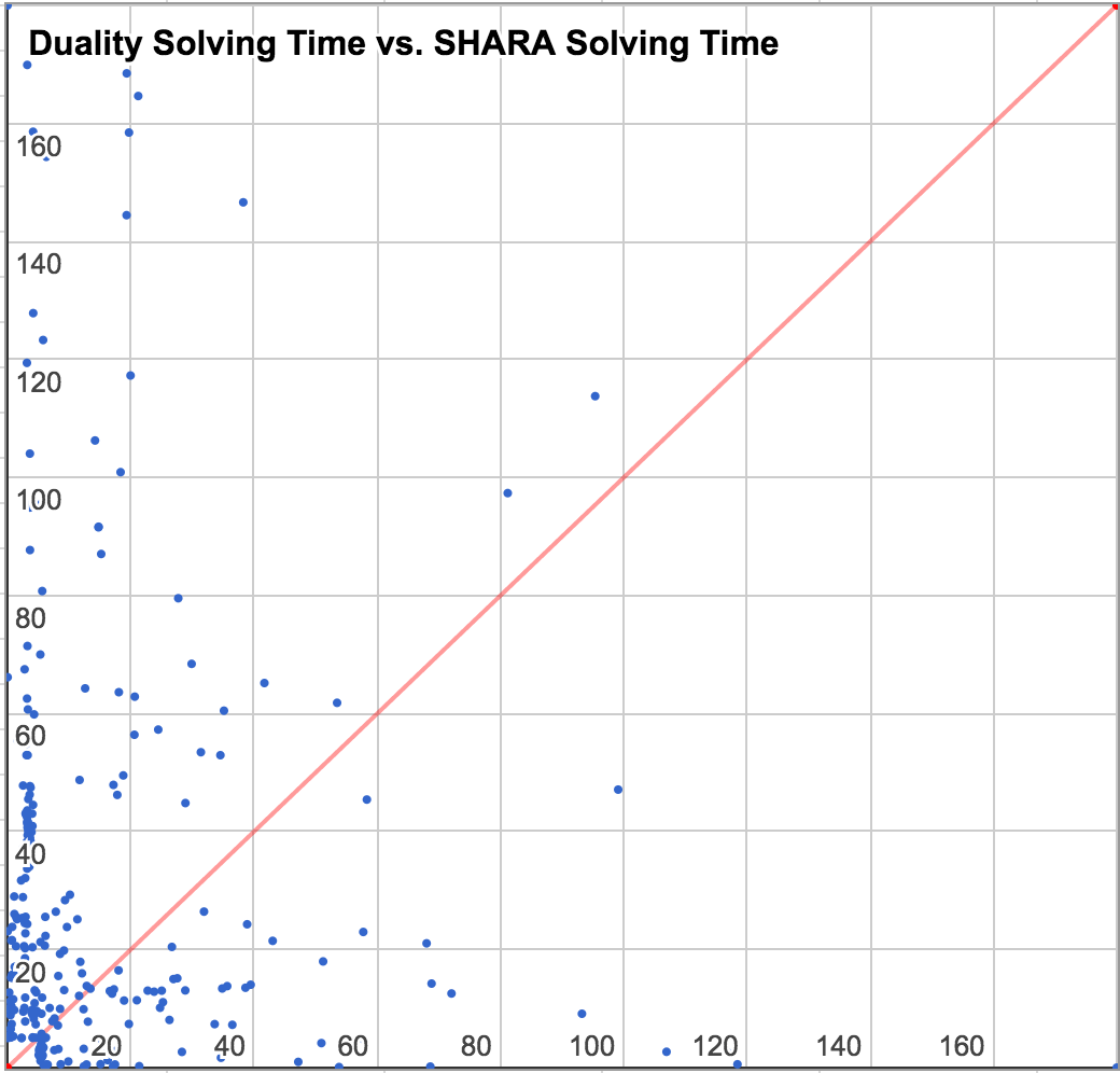
[2] [.48] [.48]

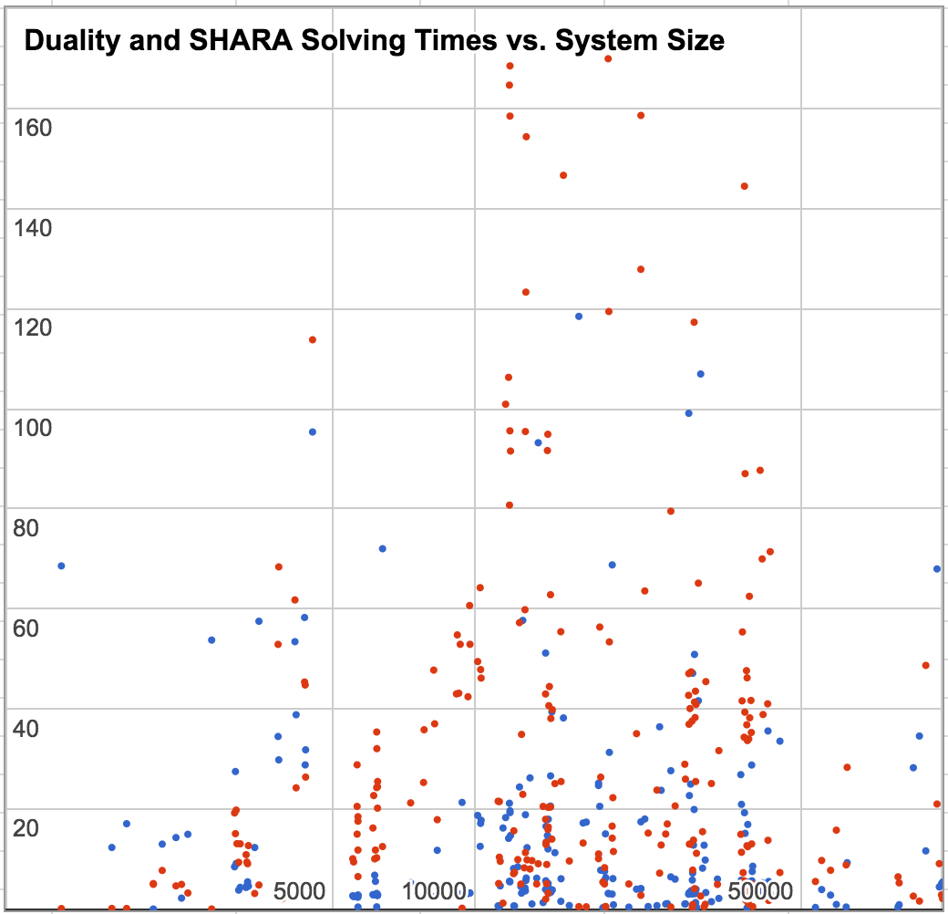
Figure 5: Solving times of Shara vs. Duality. The $x$ and $y$ axes range over the solving times in seconds of Shara and Duality, respectively. Each point depicts the performance of a benchmark. The line $y=x$ is shown in red.

Figure 6: Times of Shara and Duality vs. system size. The $x$-axis ranges over the size of a given system, and the $y$-axis ranges over solvers’ times. Measurements of Shara and Duality are shown in blue and red, respectively.

The results of our evaluation are shown in Figure 6. Of the 4,040 benchmarks on which both solvers took a short amount of time—less than five seconds—Shara solved the benchmarks in an average of 0.51 seconds and Duality solved them in an average of 0.42 seconds. Figure 6 contains data for benchmarks which took longer than five second for both systems to solve. Out of these 269 benchmarks, Shara solved 185 in less time than Duality, and solved 159 in less than half the time of Duality. Duality solved 84 in less time than Shara, and solved 53 in less than half the time of Shara. Of the 762 benchmarks on which Shara timed out, Duality solved or found a counterexample to 185. Of the 1,145 benchmarks on which Duality timed out, Shara solved or found a counterexample to 470.

Figure 6 shows the relationship between the solving times of Duality and Shara and the size of a given system, measured as lines of code in the format generated by SeaHorn. The majority of files have between 1,000 and 100,000 lines, so Figure 6 is restricted to this range. The data indicates that the performance improvement of Shara compared to Duality is consistent across systems of all sizes available.

The results indicate that (1) on a significant number of different verification problems, Shara can perform significantly better than Duality, but (2) there are some cases in which the strengths of each algorithm yield better results. Specifically, the unmodified version of Duality uses a technique called lazy annotation to avoid enumerating all derivation trees. Shara does not use lazy annotation. We collected the differences between sizes of a given system and its minimal CDD expansion generated by Shara and found that they were independent of Shara’s performance compared to Duality. Thus, while Duality may in the worst case enumerate exponentially many derivation trees, it appears to enumerate far fewer than the worst-case bound in some cases, causing it to perform better than Shara. Our results indicate that a third approach that combines the strengths of both Duality and Shara, perhaps by lazily unwinding a given system into a series of CDD systems, could yield further improvements.

6 Related Work

A significant body of previous work has presented solvers for different classes of Constrained Horn Clauses, or finding inductive invariants of programs that correspond to solutions of CHCs. Impact attempts to verify a given sequential procedure by iteratively selecting paths and synthesizing invariants for each path. This approach corresponds to solving a recursive linear CHC system [18].

Previous work also proposed a verifier for recursive programs [11]. The proposed approach selects interprocedural paths of a program and synthesizes invariants for each as nested interpolants. Such an approach corresponds to attempting to solve a recursive CHC system $S$ by selecting derivation trees of $S$ and solving each tree.

Previous work has proposed solvers for recursive systems that, given a system $S$, attempt to solve $S$ by generating and solving a series of recursion-free unwindings of $S$. In particular, Eldarica attempts to solve each unwinding $S^{\prime}$ by reducing to and solving body-disjoint systems [21, 22]. Duality attempts to avoid solving all derivation-trees (i.e body-disjoint systems) by using lazy annotation [5]. Other optimizations select derivation trees to solve using symbolic analogs of Prolog evaluation with tabling [13, 19].

Whale attempts to verify sequential recursive programs by generating and solving hierarchical programs, which correspond to recursion-free CHC systems [3]. To solve a particular recursion-free system, Whale solves a linear inlining of the input using a procedure named Vinta [2]. In general, the linear inlining may be exponentially larger than the input.

Shara is similar to the recursion-free CHC approaches given above in that it reduces the problem to solving a CHC system in a directly-solvable class. Shara is distinct in that it reduces to solving Clause-Dependent Disjoint (CDD) systems. As discussed in § 2, the class of CDD systems is a superset of classes used by the approaches above. CDD systems can also be solved directly.

Shara solves general CHC systems using the same strategy as proposed by the above approaches. Specifically, it solves a series of recursion-free unwindings of the original system, and tries to synthesize a general solution from the recursion-free solutions.

Previous work describes solvers for non-linear Horn clauses over particular theories. In particular, verifiers have been proposed for recursion-free systems over the theory of linear arithmetic [14]. Because the verifier relies on quantifier elimination, it is not clear if it can be extended to richer theories that support interpolation, such as the combination of linear arithmetic with uninterpreted functions. Other work describes a solver for the class of timed pushdown systems, a subclass of CHC systems over the theory of linear real arithmetic [12]. Unlike these approaches, Shara can solve systems over any theory that supports interpolation.

DAG inlining attempts to generate compact verification conditions for hierarchical programs [15]. Shara attempts to solve recursion-free CHC systems by reducing them to compact CDD systems. Because hierarchical programs and recursion-free CHC systems are closely related, algorithms that operate on hierarchical programs correspond to algorithms that operate on recursion-free Horn Clauses. However, it is not apparent whether such algorithms can be used directly to synthesize solutions.

Appendix A Generating a Minimal CDD Expansion

Input : A recursion-free CHC system $S$.

Output : A minimal CDD expansion $S^{\prime}$ of $S$ and a correspondence from $S^{\prime}$ to $S$.

1 Procedure $\textsc{Expand}(S)$

2       Procedure $\textsc{ExpAux}(S^{\prime})$

3             switch $\textsc{SharedRel}(S^{\prime})$ do

4                   case $\mathsf{None}$: do  return $S^{\prime}$ ;

5                    case $C\in S^{\prime},P\in\mathsf{Pred}(S^{\prime})$:  do  return $\textsc{ExpAux}(\textsc{CopyRel}(S^{\prime},C,P))$ ;

6                   

7             end switch

8            

9      

10      return $(\textsc{ExpAux}(S),\textsc{Corr})$

11

Algorithm 3 Expand: given a recursion-free CHC system $S$, returns a minimal CDD expansion $S^{\prime}$ of $S$ and its correspondence.

Given a recursion-free CHC system $S$, Alg. 3 returns a minimal CDD expansion of $S$ (Defn. 7). Expand defines a procedure ExpAux (Alg. 3—Alg. 3) that takes a CHC system $S$ and returns a minimal CDD expansion of $S$. Expand runs ExpAux on $S$ and returns the result, paired with the map $\textsc{Corr}:\mathsf{Pred}(S^{\prime})\to\mathsf{Pred}(S)$ (Alg. 3).

ExpAux, given a recursion-free CHC system $S^{\prime}$, runs a procedure SharedRel on $S^{\prime}$, which tries to find a clause $C\in S^{\prime}$ and a predicate $P\in\mathsf{Body}(C)$ such that $P$ is in the transitive dependencies of two sibling predicates. In such a case, we say that $(C,P)$ is a sibling-shared dependency.

If SharedRel determines that no sibling-shared dependency exists, then ExpAux returns $S^{\prime}$ (Alg. 3).

Otherwise, SharedRel must have located a sibling-shared dependency $(C,P)$. In this case, ExpAux runs CopyRel on $S^{\prime}$, $C$, and $P$, which returns an expansion of $S^{\prime}$ by creating a fresh copy of $P$ and updating $\mathsf{Body}(C)$ to avoid the shared dependency. ExpAux recurses on this expansion and returns the result (Alg. 3).

Expand always returns a CDD expansion of its input (see Appendix D, Lemma 3) that is minimal. Expand is certainly not unique as an algorithm for generating a minimal CDD expansion. In particular, feasible variations of Expand can be generated from different implementations of SharedRel, each of which chooses clause-relation pairs to return based on different heuristics. We expect that other expansion algorithms can also be developed by generalizing algorithms introduced in previous work on generating compact verification conditions of hierarchical programs [15].

Appendix B Proof of characterization of CDD systems

The following is a proof of Thm. 1.

Proof.

To prove that CDD is a strict superset of the union of the class of linear systems and the class of body-disjoint systems, we prove (1) CDD contains the class of linear systems, (2) CDD contains the class of body-disjoint systems, and (3) there is some CDD system that is neither linear nor body-disjoint.

For goal (1), let $S$ be an arbitrary linear system. $S$ is CDD if for each clause $C$ in $S$ (1) and each pair of distinct predicates in the body of $C$ has disjoint transitive dependencies and (2) no predicate appears more than once in the body of $C$. (Defn. 5). Let $C$ be an arbitrary clause in $S$. Since $C$ is a linear clause, it has at most one relational predicate in its body. And since the system is recursion-free, the transitive dependencies are trivially disjoint and there can be no repeated predicate. Therefore, $S$ is CDD.

For goal (2), let $S$ be an arbitrary body-disjoint system. The dependence relation of $S$ is a tree $T$, by the definition of a body-disjoint system. Let $C$ be an arbitrary clause in $S$, with distinct relational predicates $R_{\_}0$ and $R_{\_}1$ in its body. All dependencies of $R_{\_}0$ and $R_{\_}1$ are in subtrees of $T$, which are disjoint by the definition of a tree. Thus, $S$ is CDD, by Defn. 5.

For goal (3), the system $\mbox{{S}}_{\mbox{{DA}}}$ is CDD, but is neither linear nor body-disjoint. ∎

Appendix C Proof SolveCdd is in co-NP

The following is a proof of Thm. 2. Namely, SolveCdd is in co-NP.

Proof.

Pre and Post construct formulas linear in the size of the CHC system. The satisfiability problem for the constructed formulas are in NP for linear arithmetic. SolveCdd issues (at worst) a linear number of interpolation queries in terms of number of predicate. Therefore, the upper bound of SolveCdd is co-NP. ∎

Appendix D Proof of Correctness

In this section, we prove that Shara is correct when applied to recursion-free CHC systems. We first establish lemmas for the correctness of each procedure used by Shara, namely Collapse (Lemma 1 and Lemma 2), Expand (Lemma 3), and SolveCdd (Lemma 4, Lemma 6, and Lemma 7). We combine the lemmas to prove Shara is correct (Thm. 3).

For two recursion-free CHC systems $S$ and $S^{\prime}$, if $S^{\prime}$ is an expansion of $S$, then the result of collapsing a solution of $S^{\prime}$ is a solution of $S$.

Lemma 1.

For two recursion-free CHC system $S^{\prime}$ and $S$ such that $\sigma^{\prime}$ is a solution of $S^{\prime}$ and $\eta$ is a correspondence from $S^{\prime}$ to $S$, $\textsc{Collapse}(\eta,\sigma^{\prime})$ is a solution of $S$.

Proof.

For each predicate $P^{\prime}\in\mathsf{Pred}(S^{\prime})$ such that $\eta(P^{\prime})=P$, there must exist some clause $C^{\prime}\in S^{\prime}$ such that $P^{\prime}\in\mathsf{Body}(C^{\prime})$ because $S^{\prime}$ is an expansion of $S$. Let predicate $Q^{\prime}\in\mathsf{Pred}(S^{\prime})$ be the head of $C^{\prime}$. $\sigma^{\prime}[P^{\prime}]\land\mathsf{Constraint}(C^{\prime})\models\sigma^{\prime}[Q^{\prime}]$ by the fact that $\sigma^{\prime}$ is a solution of $S^{\prime}$. Therefore,

$$\textsc{Collapse}(\eta,\sigma^{\prime})[P]\land\mathsf{Constraint}(C^{\prime})\models\left(\bigwedge_{\_}{\begin{subarray}{c}Q^{\prime}\in\mathsf{Pred}(S^{\prime})\\ \eta(Q^{\prime})=Q\end{subarray}}\sigma(Q^{\prime})=\textsc{Collapse}(\eta,\sigma^{\prime})[Q^{\prime}]\right)$$

Therefore, $\textsc{Collapse}(\eta,\sigma^{\prime})$ has a solution for $P$. Since $\textsc{Collapse}(\eta,\sigma^{\prime})$ has a solution for each predicate in $S$, $\textsc{Collapse}(\eta,\sigma^{\prime})$ is a solution of $S$. ∎

Every expansion of a solvable recursion-free CHC system is also solvable.

Lemma 2.

If a recursion-free CHC system $S$ is solvable and $S^{\prime}$ is an expansion of $S$, then $S^{\prime}$ is solvable.

Proof.

Let $\sigma$ be a solution of $S$, and let $\eta$ be a correspondence from $S^{\prime}$ to $S$. Let $\sigma^{\prime}$ be such that for each $P^{\prime}\in\mathsf{Pred}(S^{\prime})$, $\sigma^{\prime}(P^{\prime})=\sigma(\eta(P^{\prime}))$. Then $\sigma^{\prime}$ is a solution of $S^{\prime}$. ∎

Expand always returns a CDD expansion of its input.

Lemma 3.

For two recursion-free CHC systems $S$ and $S^{\prime}$ and a correspondence from $S^{\prime}$ to $S$, $\eta$, such that $(S^{\prime},\eta)=\textsc{Expand}(S)$, $S^{\prime}$ is a CDD system and an expansion of $S$.

Proof.

By induction over the evaluation of Expand on an arbitrary recursion-free CHC system $S$. The inductive fact is that for each evaluation step Corr is a correspondence from argument $S^{\prime}$ to $S$. In the base case, ExpAux is called initially on $S$, by Alg. 3. Corr is a correspondence from $S$ to itself, by the definition of Corr (Appendix A).

In the inductive case, ExpAux constructs an argument $\textsc{CopyRel}(S,C,P)$ where $C$ is a clause and $P$ is a predicate in $S$. ExpAux recusively invokes itself with this argument. For each recursion-free CHC system $S^{\prime}$ generated by $\textsc{CopyRel}(S,C,P)$, Corr is a correspondence from $S^{\prime}$ to $S$ by definition of CopyRel (Appendix A). By this fact and the inductive hypothesis, Corr is a correspondence from $\textsc{CopyRel}(S^{\prime},C,P)$ to $S$.

ExpAux returns its parameter at some step, by Alg. 3. Therefore, ExpAux returns an expansion of $S$.

For a given recursion-free CHC system $S^{\prime}$, if $(S^{\prime},\eta)=\textsc{Expand}(S^{\prime})$, then $\textsc{SharedRel}(S^{\prime})=\mathsf{None}$, by the definition of Expand. If $\textsc{SharedRel}(S^{\prime})=\mathsf{None}$, then $S^{\prime}$ is CDD, by the definition of SharedRel and CDD systems (Defn. 5). Therefore, $S^{\prime}$ is CDD. ∎

Furthermore, Expand returns a minimal CDD expansion of its input. This fact is not required to prove Thm. 3, and thus a complete proof is withheld.

For each recursion-free CHC system $S$, $S$ has a solution if and only if all interpolation queries return interpolants.

Lemma 4.

Given a recursion-free CHC system $S$ that is CDD and solvable, for all predicates $P\in\mathsf{Pred}(S)$, Itp returns an interpolant $I$.

Proof.

Assume that $S$ has a solution $\sigma$ and there are some predicates $P\in\mathsf{Pred}(S)$ such that Itp returns $SAT$. This means there must be a model $m$ for the conjunction of $\textsc{Pre}(\mbox{{P}},\sigma^{\prime})$ and $\textsc{Post}(\mbox{{P}},\sigma^{\prime})$. But $\textsc{Post}(\mbox{{P}},\sigma)=\mathsf{False}$, by the definition of a solution of a CHC system. Therefore, there can be no such model $m$. Therefore, Itp always returns interpolant. ∎

Lemma 5.

Given a recursion-free CHC system $S$ that is CDD, if for all predicates $P\in\mathsf{Pred}(S)$, Itp returns an interpolant $I$, then $\textsc{SolveCdd}(S)$ is a solution of $S$.

Proof.

By induction on the $\textsc{SolveCdd}(S)$ calls to Itp over all predicates $P\in\mathsf{Pred}(S)$ in topological order. The inductive fact is that after each call to Itp, $\sigma$ is a partial solution of $S$. In the base case, $\mathsf{Pred}(S)=\varnothing$, Therefore, $\sigma$ is a solution of $S$.

In the inductive case, SolveCdd calls Itp on a predicate $P\in\mathsf{Pred}(S)$ with partial solution $\sigma$. Due to the topological ordering, $\sigma$ contains interpretations for each predicate $P\in\mathsf{Deps}(S)$. Based on the definition of an interpolant (Defn. 4), $\textsc{Pre}(\mbox{{P}},\sigma)$ and $\textsc{Post}(\mbox{{P}},\sigma)$ are inconsistent. The interpolant of these two formulas returned by Itp, $I$, is entailed by each clause $C$ where $P$ is the head where the predicates in $\mathsf{Body}(C)$ are substituted by their interpretations in $\sigma$. $I$ is also inconsistent with all constraints that appear after $P$ that support the query clause. Therefore, when SolveCdd updates $\sigma$ by binding $P$ to $I$ the result is a partial solution of $S$. ∎

The output of SolveCdd is correct for a given input CDD system.

Lemma 6.

For a given CDD system $S$, and $\sigma=\textsc{SolveCdd}(S)$, $\sigma$ is a solution of $S$.

Proof.

The fact that $\textsc{SolveCdd}(S)$ returns $\sigma$ implies that for each predicate $P\in\mathsf{Pred}(S)$, Itp returns a valid interpolant (Alg. 1). Therefore, Lemma 5 implies that SolveCdd returns a complete solution of $S$. ∎

Lemma 7.

For a CDD system $S$ such that $S$ is solvable, there is some $\sigma$ such that $\sigma=\textsc{SolveCdd}(S)$.

Proof.

For all predicates $P\in\mathsf{Pred}(S)$, Itp returns a interpolant $I$, by Lemma 4 and the fact that $S$ is solvable. Therefore, by Lemma 5 and the fact that $S$ is solvable, $\textsc{SolveCdd}(S)$ returns a solution of $S$. ∎

The output of Shara is correct for a given input CDD system. (§ 4, Thm. 3).

Proof.

Given two recursion-free CHC systems $S$ and $S^{\prime}$ and a $\eta$ such that $(S^{\prime},\eta)=\textsc{Expand}(S)$, $S^{\prime}$ is minimal CDD expansion of $S$ and $\eta$ is a correspondence from $S^{\prime}$ to $S$ (Lemma 3). Assume that $S$ is solvable. Then so is $S^{\prime}$, by Lemma 2. Therefore, there exists some $\sigma^{\prime}$ such that $\sigma^{\prime}=\textsc{SolveCdd}(S^{\prime})$, by the definition of Shara. $\sigma^{\prime}$ is a solution of $S^{\prime}$, by Lemma 6. $\textsc{Collapse}(\eta,\sigma^{\prime})$ is a solution of $S$, by Lemma 1. Therefore, Shara returns a valid solution of $S$. ∎

References

- [1]
- [2] Aws Albarghouthi, Arie Gurfinkel & Marsha Chechik (2012): Craig Interpretation. In: SAS, 10.1007/978-3-642-33125-121.
- [3] Aws Albarghouthi, Arie Gurfinkel & Marsha Chechik (2012): Whale: An Interpolation-Based Algorithm for Inter-procedural Verification. In: VMCAI, 10.1007/978-3-642-27940-94.
- [4] Aws Albarghouthi, Yi Li, Arie Gurfinkel & Marsha Chechik (2012): UFO: A Framework for Abstraction- and Interpolation-Based Software Verification. In: CAV, 10.1007/978-3-642-31424-748.
- [5] Nikolaj Bjørner, Kenneth L. McMillan & Andrey Rybalchenko (2013): On Solving Universally Quantified Horn Clauses. In: SAS, 10.1007/978-3-642-38856-98.
- [6] Cormac Flanagan (2003): Automatic Software Model Checking Using CLP. In: ESOP, 10.1007/3-540-36575-314.
- [7] Cormac Flanagan & James B. Saxe (2001): Avoiding exponential explosion: generating compact verification conditions. In: POPL, 10.1145/360204.360220.
- [8] (2016): GitHub - sosy-lab/sv-benchmarks: svcomp15. https://github.com/sosy-lab/sv-benchmarks/releases/tag/svcomp15. Accessed: 2016 Dec 13.
- [9] (2016): GitHub - Z3Prover/z3: The Z3 Theorem Prover. https://github.com/Z3Prover/z3. Accessed: 2016 Dec 13.
- [10] Arie Gurfinkel, Temesghen Kahsai, Anvesh Komuravelli & Jorge A. Navas (2015): The SeaHorn Verification Framework. In: CAV, 10.1007/978-3-319-21690-420.
- [11] Matthias Heizmann, Jochen Hoenicke & Andreas Podelski (2010): Nested interpolants. In: POPL, 10.1145/1706299.1706353.
- [12] Krystof Hoder & Nikolaj Bjørner (2012): Generalized Property Directed Reachability. In: SAT, 10.1007/978-3-642-31612-813.
- [13] Joxan Jaffar, Andrew E. Santosa & Razvan Voicu (2009): An Interpolation Method for CLP Traversal. In: CP, 10.1007/978-3-642-04244-737.
- [14] Anvesh Komuravelli, Arie Gurfinkel & Sagar Chaki (2014): SMT-Based Model Checking for Recursive Programs. In: CAV, 10.1007/978-3-319-08867-92.
- [15] Akash Lal & Shaz Qadeer (2015): DAG inlining: a decision procedure for reachability-modulo-theories in hierarchical programs. In: PLDI, 10.1145/2813885.2737987.
- [16] Akash Lal, Shaz Qadeer & Shuvendu K. Lahiri (2012): A Solver for Reachability Modulo Theories. In: CAV, 10.1007/978-3-642-31424-732.
- [17] Kenneth L. McMillan (2004): An Interpolating Theorem Prover. In: TACAS, 10.1016/j.tcs.2005.07.003.
- [18] Kenneth L. McMillan (2006): Lazy Abstraction with Interpolants. In: CAV, 10.1007/1181796314.
- [19] Kenneth L. McMillan (2014): Lazy Annotation Revisited. In: CAV, 10.1007/978-3-319-08867-916.
- [20] Leonardo Mendonça de Moura & Nikolaj Bjørner (2008): Z3: An Efficient SMT Solver. In: TACAS, 10.1007/978-3-540-78800-324.
- [21] Philipp Rümmer, Hossein Hojjat & Viktor Kuncak (2013): Classifying and Solving Horn Clauses for Verification. In: VSTTE, 10.1007/978-3-642-54108-71.
- [22] Philipp Rümmer, Hossein Hojjat & Viktor Kuncak (2013): Disjunctive Interpolants for Horn-clause Verification. In: CAV, 10.1007/978-3-642-39799-824.