Figure 1. Our proposed method colorizes a grayscale image (left), guided by sparse user inputs (second), in real-time, providing the capability for quickly generating multiple plausible colorizations (middle to right). Photograph of Migrant Mother by Dorothea Lange, 1936 (Public Domain).

Real-Time User-Guided Image Colorization with Learned Deep Priors

Abstract.

We propose a deep learning approach for user-guided image colorization. The system directly maps a grayscale image, along with sparse, local user “hints” to an output colorization with a Convolutional Neural Network (CNN). Rather than using hand-defined rules, the network propagates user edits by fusing low-level cues along with high-level semantic information, learned from large-scale data. We train on a million images, with simulated user inputs. To guide the user towards efficient input selection, the system recommends likely colors based on the input image and current user inputs. The colorization is performed in a single feed-forward pass, enabling real-time use. Even with randomly simulated user inputs, we show that the proposed system helps novice users quickly create realistic colorizations, and offers large improvements in colorization quality with just a minute of use. In addition, we demonstrate that the framework can incorporate other user “hints” to the desired colorization, showing an application to color histogram transfer. Our code and models are available at https://richzhang.github.io/ideepcolor.

1. Introduction

There is something uniquely and powerfully satisfying about the simple act of adding color to black and white imagery. Whether as a way of rekindling old, dormant memories or expressing artistic creativity, people continue to be fascinated by colorization. From remastering classic black and white films, to the enduring popularity of coloring books for all ages, to the surprising enthusiasm for various (often not very good) automatic colorization bots online, this topic continues to fascinate the public.

In computer graphics, two broad approaches to image colorization exist: user-guided edit propagation and data-driven automatic colorization. In the first paradigm, popularized by the seminal work of Levin et al. (2004), a user draws colored strokes over a grayscale image. An optimization procedure then generates a colorized image that matches the user’s scribbles, while also adhering to hand-defined image priors, such as piecewise smoothness. These methods can achieve impressive results but often require intensive user interaction (sometimes over fifty strokes), as each differently colored image region must be explicitly indicated by the user. Because the system purely relies on user inputs for colors, even regions with little color uncertainty, such as green vegetation, need to be specified. Less obviously, even if a user knows what general color an object should take on, it can be surprisingly difficult to select the exact desired natural chrominance.

To address these limitations, researchers have also explored more data-driven colorization methods. These methods colorize a grayscale photo in one of two ways: either by matching it to an exemplar color image in a database and non-parametrically “stealing” colors from that photo, an idea going back to Image Analogies (Hertzmann et al., 2001), or by learning parametric mappings from grayscale to color from large-scale image data. The most recent methods in this paradigm proposed by Iizuka et al. (2016), Larsson et al. (2016), and Zhang et al. (2016), use deep networks and are fully automatic. Although this makes colorizing a new photo cheap and easy, the results often contain incorrect colors and obvious artifacts. More fundamentally, the color of an object, such as a t-shirt, is often inherently ambiguous – it could be blue, red, or green. Current automatic methods aim to choose a single colorization, and do not allow a user to specify their preference for a plausible, or perhaps artistic, alternative.

Might we be able to get the best of both worlds, leveraging large-scale data to learn priors about natural color imagery, while at the same time incorporating user control from traditional edit propagation frameworks? We propose to train a CNN to directly map grayscale images, along with sparse user inputs, to an output colorization. During training, we randomly simulate user inputs, allowing us to bypass the difficulty of collecting user interactions. Though our network is trained with ground truth natural images, the network can colorize objects with different, or even unlikely colorizations, if desired.

Most traditional tools in interactive graphics are defined either procedurally – e.g., as a designed image filter – or as constraints applied in a hand-engineered optimization framework. The behavior of the tool is therefore fully specified by human fiat. This approach is fundamentally limited by the skill of engineers to design complex operations/constraints that actually accomplish what is intended of them. Our approach differs in that the effect of interaction is learned. Through learning, the algorithm may come up with a more powerful procedure for translating user edits to colorized results than would be feasible by human design.

Our contribution are as follows: (1) We end-to-end learn how to propagate sparse user points from large-scale data, by training a deep network to directly predict the mapping from grayscale image and user points to full color image. (2) To guide the user toward making informed decisions, we provide a data-driven color palette, which suggests the most probable colors at any given location. (3) We run a study, showing that even given minimal training with our interface and limited time to colorize an image (1 min), novice users can quickly learn to produce colorizations that can often fool real human judges in a real vs. fake test. (4) Though our system is trained on natural images, it can also generate unusual colorizations. (5) We demonstrate that this framework is not limited to user points, and can, in principle, be trained with any statistic of the output, for example, global color distribution or average image saturation.

Figure 2. Network architecture We train two variants of the user interaction colorization network. Both variants use the blue layers for predicting a colorization. The Local Hints Network also uses red layers to (a) incorporate user points $\mathbf{U}_{l}$ and (b) predict a color distribution $\mathbf{\widehat{Z}}$. The Global Hints Network uses the green layers, which transforms global input $\mathbf{U}_{g}$ by $1\times 1$ conv layers, and adds the result into the main colorization network. Each box represents a conv layer, with vertical dimension indicating feature map spatial resolution, and horizontal dimension indicating number of channels. Changes in resolution are achieved through subsampling and upsampling operations. In the main network, when resolution is decreased, the number of feature channels are doubled. Shortcut connections are added to upsampling convolution layers.

2. Related Work

User-guided colorization

Prior interactive colorization work focused on local control, such as user strokes (Levin et al., 2004; Huang et al., 2005). Because the strokes are propagated using low-level similarity metrics, such as spatial offset and intensity difference, numerous user edits are typically required to achieve realistic results. To reduce user efforts, later methods focused on designing better similarity metrics (Qu et al., 2006; Luan et al., 2007) and utilizing long-range connections (An and Pellacini, 2008; Xu et al., 2009). Learning machinery, such as boosting (Li et al., 2008), local linear embeddings (Chen et al., 2012), feature discrimination (Xu et al., 2013), and more recently, neural networks (Endo et al., 2016), have been proposed to automatically learn similarity between pixels given user strokes and input images. In addition to local control, varying the color theme (Wang et al., 2010; Li et al., 2015) and color palette (Chang et al., 2015) are popular methods of expressive global control. We show that we can integrate global hints to our network and control colorization results by altering the color distribution and average saturation (see Section 3.3). Concurrently, Sangkloy et al. (2017) developed a system to translate sketches to real images, with support for user color strokes, while PaintsChainer (2017) and Frans  (2017) have developed open-source interactive online applications for line-drawing colorization.

Automatic colorization

Early semi-automatic methods (Welsh et al., 2002; Irony et al., 2005; Liu et al., 2008; Chia et al., 2011; Gupta et al., 2012) utilize an example-based approach that transfers color statistics from a reference image or multiple images (Morimoto et al., 2009; Liu et al., 2014) to the input grayscale image with techniques such as color transfer (Reinhard et al., 2001) and image analogies (Hertzmann et al., 2001). These methods work remarkably well when the input and the reference share similar content. However, finding reference images is time-consuming and can be challenging for rare objects or complex scenes, even when using semi-automatic retrieval methods (Chia et al., 2011). In addition, some algorithms  (Irony et al., 2005; Chia et al., 2011) involve tedious manual efforts on defining corresponding regions between images.

Recently, fully automatic methods (Deshpande et al., 2015; Cheng et al., 2015; Iizuka et al., 2016; Zhang et al., 2016; Larsson et al., 2016; Isola et al., 2017) have been proposed. The recent methods from train CNNs (LeCun et al., 1998) on large-scale image collections (Russakovsky et al., 2015; Zhou et al., 2014) to directly map grayscale images to output colors. The networks can learn to combine low and high-level cues to perform colorization, and have been shown to produce realistic results, as determined by human judgments (Zhang et al., 2016). However, these approaches aim to produce a single plausible result, even though colorization is intrinsically an ill-posed problem with multi-modal uncertainty (Charpiat et al., 2008). Larsson et al. (2016) provide some post-hoc control through globally biasing the hue, or by matching global statistics to a target histogram. Our work addresses this problem by learning to integrate input hints in an end-to-end manner.

Deep semantic image editing

Deep neural networks (Krizhevsky et al., 2012) excel at extracting rich semantics from images, from middle-level concepts like material (Bell et al., 2015; Wang et al., 2016) and segmentation (Xie and Tu, 2015), to high-level knowledge such as objects (Girshick et al., 2014) and scene categories (Zhou et al., 2014). All of this information could potentially benefit semantic image editing, i.e. changing the high-level visual content with minimal user interaction. Recently, neural networks have shown impressive results for various image processing tasks, such as photo enhancement (Yan et al., 2016), sketch simplification (Simo-Serra et al., 2016), style transfer (Gatys et al., 2016; Selim et al., 2016), inpainting (Pathak et al., 2016), image blending (Zhu et al., 2015) and denoising (Gharbi et al., 2016). Most of these works built image filtering pipelines and trained networks that produce a filtered version of the input image with different low-level local details. However, none of these methods allowed dramatic, high-level modification of the visual appearance, nor do they provide diverse outputs in a user controllable fashion. On the contrary, we train a network that takes an input image as well as minimal user guidance and produces global changes in the image with a few clicks. Barnes et al. (2009) emphasize that control and interactivity are key to image editing, because user intervention not only can correct errors, but can also help explore the vast design space of creative image manipulation. We incorporate this concept into an intuitive interface that provides expressive controls as well as real-time feedback. Zhu et al.  (2016) provided an interactive deep image synthesis interface that builds on an image prior learned by a deep generative network. Xu et al. (2016) train a deep network for interactive object segmentation. Isola et al. (2017) and Sangkloy et al. (2017) train networks to generate images from sketches, using synthetic sketches generated by edge detection algorithms for training data.

3. Methods

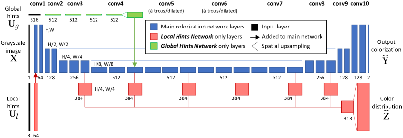
We train a deep network to predict the color of an image, given the grayscale version and user inputs. In Section 3.1, we describe the objective of the network. We then describe the two variants of our system (i) the Local Hints Network in Section 3.2, which uses sparse user points, and (ii) the Global Hints Network in Section 3.3, which uses global statistics. In Section 3.4, we define our network architecture.

3.1. Learning to Colorize

The inputs to our system are a grayscale image $\mathbf{X}\in\mathds{R}^{H\times W\times 1}$, along with an input user tensor $\mathbf{U}$. The grayscale image is the $L$, or lightness in the CIE $Lab$ color space, channel. The output of the system is $\mathbf{\widehat{Y}}\in\mathds{R}^{H\times W\times 2}$, the estimate of the $ab$ color channels of the image. The mapping is learned with a CNN $\mathcal{F}$, parameterized by $\theta$, with the network architecture specified in Section 3.4 and shown in Figure 2. We train the network to minimize the objective function in Equation 1, across $\mathcal{D}$, which represents a dataset of grayscale images, user inputs, and desired output colorizations. Loss function $\mathcal{L}$ describes how close the network output is to the ground truth.

(1) $$\mathcal{\theta}^{*}=\arg\min_{\mathcal{\theta}}\mathds{E}_{\mathbf{X},\mathbf{U},\mathbf{Y}\sim\mathcal{D}}[\mathcal{L}(\mathcal{F}(\mathbf{X},\mathbf{U};\theta),\mathbf{Y})]\\$$

We train two variants of our network, with local user hints $\mathbf{U}_{l}$ and global user hints $\mathbf{U}_{g}$. During training, the hints are generated by giving the network a “peek”, or projection, of the ground truth color $\mathbf{Y}$ using functions $\mathcal{P}_{l}$ and $\mathcal{P}_{g}$, respectively.

(2) $$\mathbf{U}_{l}=\mathcal{P}_{l}(\mathbf{Y})\hskip 28.45274pt\mathbf{U}_{g}=\mathcal{P}_{g}(\mathbf{Y})$$

The minimization problems for the Local and Global Hints Networks are then described below in Equation 3. Because we are using functions $\mathcal{P}_{l},\mathcal{P}_{g}$ to synethtically generate user inputs, our dataset only needs to contain grayscale and color images. We use the 1.3M ImageNet dataset (Russakovsky et al., 2015).

(3) $$\begin{split}&\mathcal{\theta}^{*}_{l}=\arg\min_{\mathcal{\theta}_{l}}\mathds{E}_{\mathbf{X},\mathbf{Y}\sim\mathcal{D}}[\mathcal{L}(\mathcal{F}_{l}(\mathbf{X},\mathbf{U}_{l};\theta_{l}),\mathbf{Y})]\\ &\mathcal{\theta}^{*}_{g}=\arg\min_{\mathcal{\theta}_{g}}\mathds{E}_{\mathbf{X},\mathbf{Y}\sim\mathcal{D}}[\mathcal{L}(\mathcal{F}_{g}(\mathbf{X},\mathbf{U}_{g};\theta_{g}),\mathbf{Y})]\end{split}$$

Figure 3. Suggested Palette Our interface provides suggested colors for any pixel, sorted by likelihood, based on the predicted color distribution given by our network. In this example, we show first suggested colors on the background vegetation (top palette), sorted by decreasing likelihood. The suggested colors are common colors for vegetation. We also show the top six suggested colors (bottom palette) of a pixel on the image of the bird. On the right, we show the resulting colorizations, based on the user selecting these top six suggested colors. Photograph of blue-and-yellow macaw by Luc Viatour, 2009.

Loss Function

The choice of an appropriate loss function $\mathcal{L}$, which measures network performance and guides learning, requires some consideration. Iizuka et al. (2016) use an $\ell_{2}$ loss. Previous work (Zhang et al., 2016; Larsson et al., 2016; Charpiat et al., 2008) note that this loss is not robust to the inherent multi-modal nature of the problem, and instead use a classification loss, followed by a fixed inference step. Another challenge is the large imbalance in natural image statistics, with many more pixels in desaturated regions of the color gamut. This can often lead to desaturated and dull colorizations. Zhang et al. (2016) use a class-rebalancing step to oversample more colorful portions of the gamut during training. This results in more colorizations which are vibrant and able to fool humans, but at the expense of images which are over-aggressively colorized. In the pix2pix framework, Isola et al. (2017) use an $\ell_{1}$ regression loss with a Generative Adversarial Network (GAN) (Goodfellow et al., 2014) term, which can help generate exciting, higher frequency patterns.

However, in our work, we forgo the use of class rebalancing from (Zhang et al., 2016) and GAN term from  (Isola et al., 2017) and use a smooth-$\ell_{1}$ (or Huber) loss, described in Equation 4. In the Local Hints Network, from a user experience standpoint, we found it more pleasing to start with a conservative colorization and allow the user to inject desired colors, rather than starting with a more vibrant but artifact-prone setting and having the user fix mistakes. Much of the multi-modal ambiguity of the problem is quickly resolved by a few user clicks. In cases where there is ambiguity, the smooth-$\ell_{1}$ is also a robust estimator (Huber, 1964), which can help avoid the averaging problem. In addition, using a regression loss, described in Equation 4 with $\delta=1$, enables us to perform end-to-end learning without a fixed inference step.

(4) $$\ell_{\delta}(x,y)=\tfrac{1}{2}(x-y)^{2}\mathds{1}_{\big{\{}|x-y|<\delta\big{\}}}+\delta(|x-y|-\tfrac{1}{2}\delta)\mathds{1}_{\big{\{}|x-y|\geq\delta\big{\}}}$$

The loss function $\ell_{\delta}$ is evaluated at each pixel and summed together to evaluate the loss $\mathcal{L}$ for a whole image.

(5) $$\mathcal{L}(\mathcal{F}(\mathbf{X},\mathbf{U};\theta),\mathbf{Y})=\sum_{h,w}\sum_{q}\ell_{\delta}\big{(}\mathcal{F}(\mathbf{X,U};\theta)_{h,w,q},\mathbf{Y}_{h,w,q}\big{)}$$

Next, we describe the specifics of the local and global variants.

3.2. Local Hints Network

The Local Hints Network uses sparse user points as input. We describe the input, how we simulate user points, and features of our user interface.

System Input

The user points are parameterized as $\mathbf{X}_{ab}\in\mathds{R}^{H\times W\times 2}$, a sparse tensor with $ab$ values for the points provided by the user and $\mathbf{B}_{ab}\in\mathds{B}^{H\times W\times 1}$, a binary mask indicating which points are provided by the user. The mask differentiates unspecified points from user-specified gray points with $(a,b)=0$. Together, the tensors form input tensor $\mathbf{U}_{l}=\{\mathbf{X}_{ab},\mathbf{B}_{ab}\}\in\mathds{R}^{H\times W\times 3}$.

Simulating User Interactions

One challenge in training deep networks is collecting training data. While data for automatic colorization is readily available – any color image can be broken up into its color and grayscale components – an appropriate mechanism for acquiring user interaction data is far less obvious. Gathering this on a large scale is not only expensive, but also comes with a chicken and egg problem, as user interaction behavior will be dependent on the system performance itself. We bypass this issue by training with synthetically generated user interactions. A concern with this approach is the potential domain gap between the generated data and test-time usage. However, we found that even through randomly sampling, we are able to cover the input space adequately and train an effective system.

We sample small patches and reveal the average patch color to the network. For each image, the number of points are drawn from a geometric distribution with $p=\tfrac{1}{8}$. Each point location is sampled from a 2-D Gaussian with $\mu=\tfrac{1}{2}[H,W]^{T},\Sigma=diag\big{(}\big{[}\big{(}\tfrac{H}{4}\big{)}^{2},\big{(}\tfrac{W}{4}\big{)}^{2}\big{]}\big{)}$, as we expect users to more often click on points in the center of the image. The revealed patch size is drawn uniformly from size $1\times 1$ to $9\times 9$, with the average $ab$ within the patch revealed to the network. Lastly, we desire the correct limiting characteristic – given all of the points by the user, the network should simply copy the colors from the input to the output. To encourage this, we provide the full ground truth color to the image for 1% of the training instances. Though the network should implicitly learn to copy any provided user points to the output, there is no explicit constraint for the network to do so exactly. Note that these design decisions for projection function $\mathcal{P}_{l}(\mathbf{Y})$ were initially selected based on intuition, found to work well, but not finely tuned.

User interface

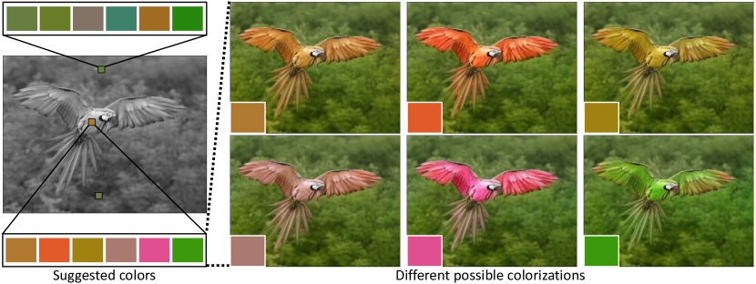
Our interface consists of a drawing pad, showing user points overlaid on the grayscale input image, a display updating the colorization result in real-time, a data-driven color palette that suggests likely color for a given location (as shown in Figure 3), and a regular $ab$ gamut based on the lightness of the current point. A user is always free to add, move, delete, or change the color of any existing points. Please see our supplemental video for a detailed introduction of our interface, along with several demonstrations.

Data-driven color palette

Picking a plausible color is an important step towards realistic colorization. Without the proper tools, selecting a color can be difficult for a novice user to intuit. For every pixel, we predict a probability distribution over output colors $\mathbf{\widehat{Z}}\in\mathds{R}^{H\times W\times Q}$, where $Q$ is the number of quantized color bins. We use the parametrization of the CIE $Lab$ color space from Zhang et al. (2016) – the $ab$ space is divided into $10\times 10$ bins, and the $Q=313$ bins that are in-gamut are kept. The mapping from the input grayscale image and user points to predicted color distribution $\mathbf{\widehat{Z}}$ is learned with network $\mathcal{G}_{l}$, parametrized by $\psi_{l}$. Ground truth distribution $\mathbf{Z}$ is encoded from ground truth colors $\mathbf{Y}$ with the soft-encoding scheme from (Zhang et al., 2016) – a real $ab$ color value is expressed as a convex combination of its 10 nearest bin centers, weighted by a Gaussian kernel with $\sigma=5$. We use a cross-entropy loss function for every pixel to measure the distance between predicted and ground truth distributions, and sum over all pixels.

(6) $$\mathcal{L}_{cl}(\mathcal{G}_{l}(\mathbf{X,U}_{l};\psi_{l}),\mathbf{Z})=-\sum_{h,w}\sum_{q}\mathbf{Z}_{h,w,q}\log(\mathcal{G}_{l}(\mathbf{X,U}_{l};\psi_{l})_{h,w,q})$$

Network $\mathcal{G}_{l}$ is trained to minimize expected classification loss over the training set. We further describe the network architecture in Section 3.4.

(7) $$\psi_{l}^{*}=\arg\min_{\psi_{l}}\mathds{E}_{\mathbf{X},\mathbf{Y}\sim\mathcal{D}}[\mathcal{L}_{cl}(\mathcal{G}_{l}(\mathbf{X,U}_{l};\psi_{l}),\mathbf{Y})]\\$$

To provide discrete color suggestions, we soften the softmax distribution at the queried pixel, to make it less peaky, and perform weighted k-means clustering (with $K=9$) to find modes of the distribution. For example, the system often recommends plausible colors based on the type of object, material and texture, for example, suggesting different shades of green the vegetation in Figure 3. For objects with diverse colors such as a parrot, our system will provide a wide range of suggestions. Once a user selects a suggested color, our system will produce the colorization result in real-time. In Figure 3, we show six possible colorizations based on the different choices for the parrot’s feather. The color suggestions are continuously updated as the user adds additional points.

Figure 4. User study results These results are collected from novice users using our Local Hints Network system for 1 minute for each image, with minimal training. Users were not given the ground truth image, and were instructed to create a “realistic colorization”. The first column shows the grayscale input image. Columns 2-5 show automatic results from previous methods, as well as our system without user points. Column 6 shows input points from a user, collected in 1 minute of time from a novice user. Columns 7-8 show the results from the seminal method of (Levin et al., 2004) and our model, incorporating user points, on the right. The final column shows the ground truth image (which was not provided to the user). In the selected examples in rows 1-4, our system produces higher quality colorizations given sparse inputs than (Levin et al., 2004), and produce nearly photorealistic results given little user interaction. Rows 5-6 show some failures of our system. In row 5, the green color by the user on the top-right is not successfully propagated to the top-left of the image. In row 6, the colors selected on the jeans are propagated to the background, demonstrating undesired non-local effects. All of the user study results are publicly available on https://richzhang.github.io/ideepcolor/. Images are from the ImageNet dataset (Russakovsky et al., 2015).

Figure 5. Selected User Study Results We show grayscale images with user inputs, alongside the output from our algorithm. Each image was colorized in only 1 minute of time by a novice user. All of the user study results are publicly available on https://richzhang.github.io/ideepcolor/. Images are from the Imagenet dataset (Russakovsky et al., 2015).

3.3. Global Hints Network

An advantage of the end-to-end learning framework is that it may be easily adapted to different types of user inputs. We show an additional use case, where the user provides global statistics, described by a global histogram $\mathbf{X}_{hist}\in\Delta^{Q}$ and average image saturation $\mathbf{X}_{sat}\in[0,1]$. Whether or not the inputs are provided is indexed by indicator variables $\mathbf{B}_{hist},\mathbf{B}_{sat}\in\mathds{B}$, respectively. The user input to the system is then $\mathbf{U}_{g}=\{\mathbf{X}_{hist},\mathbf{B}_{hist},\mathbf{X}_{sat},\mathbf{B}_{sat}\}\in\mathds{Re}^{1\times 1\times(Q+3)}$.

We compute global histograms by resizing the color $\mathbf{Y}$ to quarter resolution using bilinear interpolation, encoding each pixel in quantized $ab$ space, and averaging spatially. Saturation is computed by converting the ground truth image to HSV colorspace and averaging over the S channel spatially. We randomly reveal the ground truth colorization distribution, ground truth saturation, both, or neither, to the network during training.

3.4. Network Architecture

We show our network architecture in Figure 2. The main colorization branch is used by both Local Hints and Global Hints networks. We then describe the layers which are only used for the Local Hints Network, namely processing the sparse user input $\mathbf{U}_{l}$ and the color distribution prediction branch, both shown in red. Finally, we describe the Global Hints Network-specific input branch, shown in green, as well as its integration in the main network.

3.4.1. Main colorization network

The main branch of our network, $\mathcal{F}$, uses a U-Net architecture (Ronneberger et al., 2015), which has been shown to work well for a variety of conditional generation tasks (Isola et al., 2017). We also utilize design principles from (Simonyan and Zisserman, 2014) and (Yu and Koltun, 2016). The network is formed by 10 convolutional blocks, conv1-10. In conv1-4, in every block, feature tensors are progressively halved spatially, while doubling in the feature dimension. Each block contains 2-3 conv-relu pairs. In the second half, conv7-10, spatial resolution is recovered, while feature dimensions are halved. In block conv5-6, instead of halving the spatial resolution, dilated convolutions with factor 2 is used. This has an equal effect on the receptive field of each unit with respect to the input pixels, but allows the network to keep additional information in the bottleneck. Symmetric shortcut connections are added to help the network recover spatial information (Ronneberger et al., 2015). For example, the conv2 and conv3 blocks are connected to the conv8 and conv9 blocks, respectively. This also enables easy accessibility to important low-level information for later layers; for example, the lightness value will limit the extent of the $ab$ gamut. Changes in spatial resolution are achieved using subsampling or upsampling operations, and each convolution uses a $3\times 3$ kernel. BatchNorm layers are added after each convolutional block, which has been shown to help training.

A subset of our network architecture, namely conv1-8 without the shortcut connections, was used by Zhang et al. (2016). For these layers, we fine-tune from these pre-trained weights. The added conv9, conv10 layers and shortcut connections are trained from scratch. A last conv layer, which is a $1\times 1$ kernel, maps between conv10 and the output color. Because the $ab$ gamut is bounded, we add a final tanh layer on the output, as is common practice when generating images (Goodfellow et al., 2014; Zhu et al., 2016).

3.4.2. Local Hints Network

The layers specific to the Local Hints Network are shown in red in Figure 2. Sparse user points are integrated by concatenation with the input grayscale image. As a side task, we also predict a color distribution at each pixel (conditioned on the grayscale and user points) to recommend to the user. The task of predicting a color distribution is undoubtedly related to the task of predicting a single colorization, so we reuse features from the main branch. We use a hypercolumn approach (Hariharan et al., 2015; Larsson et al., 2016) by concatenating features from multiple layers of the main branch, and learning a two-layer classifier on top. Network $\mathcal{G}_{l}$ is composed of the main branch, up to conv8, along with this side branch. The side task should not affect the main task’s representation, so we do not back-propagate the gradients from the side task into the main branch. To save computation, we predict the distribution at a quarter resolution, and apply bilinear upsampling to predict at full resolution.

3.4.3. Global Hints Network

Because the global inputs have no spatial information, we choose to integrate the information into the middle of the main colorization network. As shown in the top green branch in Figure 2, the inputs are processed through 4 conv-relu layers, with kernel size $1\times 1$ and 512 channels each. This feature map is repeated spatially to match the size of the conv4 feature in the main branch, $\mathds{R}^{\nicefrac{{H}}{{8}}\times\nicefrac{{W}}{{8}}\times 512}$, and merged by summation, a similar strategy to the one used by Iizuka et al. (2016).

Figure 6. Average PSNR vs Number of Revealed Points We measure the average PSNR from our ImageNet test set across different algorithms. Points are revealed to each algorithm by random or max-error sampling. Max-error sampling selects the point with maximum $\ell_{2}$ error in $ab$ space between predicted and ground truth. Random sampling uses a uniformly drawn random point. The average color on a $7\times 7$ patch is revealed to the algorithm. The x-axis is on a logarithmic scale. Baselines (Levin et al., 2004; Barron and Poole, 2016; Endo et al., 2016) are computed with publicly available code from the authors. Because our algorithm is learned on a large-scale corpus of data, our system provides more accurate colorizations given little user supervision. With large amounts of input points (approximately 500 for random sampling), (Levin et al., 2004) begins to achieve equal accuracy to ours. For reference, we show our network without user inputs, Ours (auto), and predicting Gray for every pixel.

4. Experiments

We detail qualitative and quantitative experiments with our system. In Section 4.1, we first automatically test the Local Hints Network. We then describe our user study in Section 4.2. The results suggest that even with little training and just 1 minute to work with an image, novice users can quickly create realistic colorizations. In Section 4.3, we show qualitative examples on unusual colorizations. In Section 4.4 we evaluate our Global Hints Network. In Section 4.5, we investigate how the Local Hints Network reconciles two colors within a single segment. Finally, we show qualitative examples on legacy grayscale images in Section 4.6.

Method	Added Inputs	PSNR (dB)
Predict gray	–	22.82$\pm$0.18
Zhang et al. (2016)	automatic	22.04$\pm$0.11
Zhang et al. (2016) (no-rebal)	automatic	24.51$\pm$0.15
Larsson et al. (2016)	automatic	24.93$\pm$0.14
Iizuka et al. (2016)	automatic	23.69$\pm$0.13
Ours (Local)	automatic	24.43$\pm$0.14
Ours (Global)	+ global hist	27.85$\pm$0.13
Ours (Global)	+ global sat	25.78$\pm$0.15
Ours (Local)	+ gt colors	37.70$\pm$0.14
Edit propagation	+ gt colors	$\infty$

Table 1. PSNR with added information. Run on 1000 held-out test images, in the ILSVRC2012 (Russakovsky et al., 2015) validation dataset. Ours (Local)-automatic is run completely automatically, with no user inputs. Methods (Zhang et al., 2016; Larsson et al., 2016; Iizuka et al., 2016) are recently automatic colorization methods. Even though our network is trained primarily for interactive colorization, it performs competitively for automatic colorization as well by this metric. Ours (Global) +global hist provides global distribution of colors in the $ab$ gamut; Ours (Global) +global sat provides global saturation to the system. Our Global Hints Network learns to incorporate global statistics for more accurate colorizations.

4.1. How well does the system incorporate inputs?

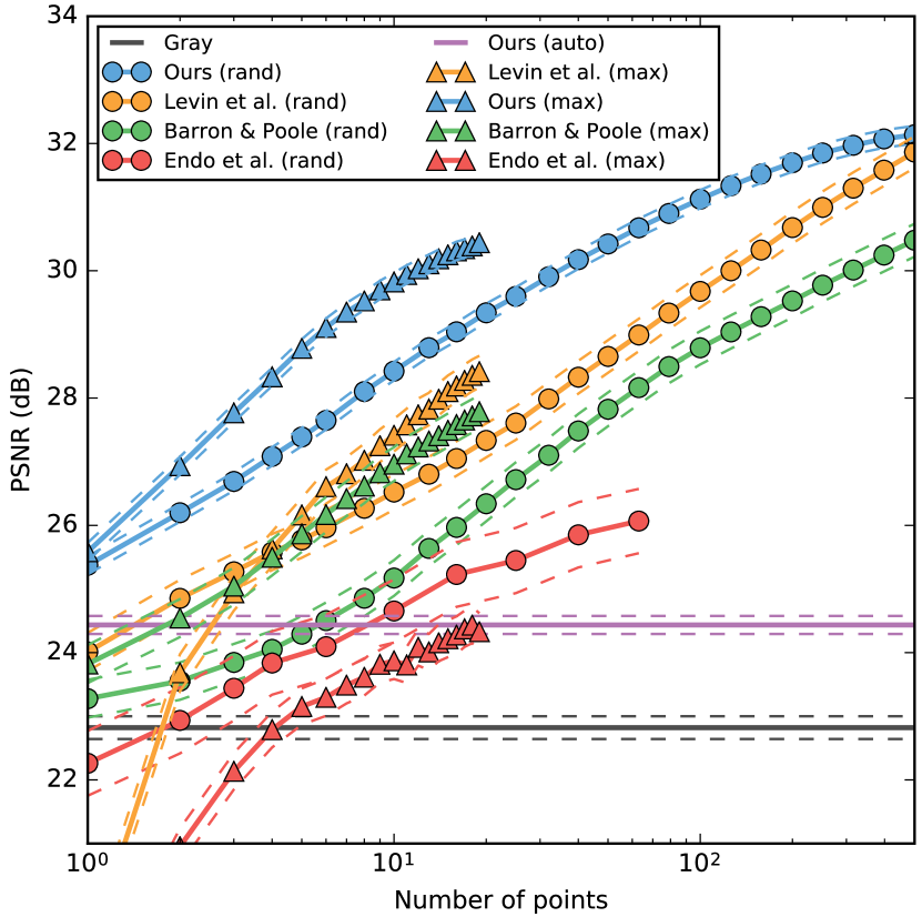
We test the system automatically by randomly revealing patches to the algorithm, and measuring PSNR, as shown in Figure 6. The pitfalls of using low-level or per-pixel metrics have been discussed in the automatic colorization regime (Zhang et al., 2016). A system which chooses a plausible but different mode than the ground truth color will be overly penalized, and may even achieve a lower score than an implausible but neutral colorization, such as predicting gray for every pixel (PSNR 22.8). In this context, however, since ground truth colors are revealed to the algorithm, the problem is much more constrained, and PSNR is a more appropriate metric.

With no revealed information, edit propagation methods will default to gray for the whole image. Our system will perform automatic colorization, and provide its best estimate (PSNR 24.4), as described in Table 1. As points are revealed, PSNR incrementally increases across all methods. Our method achieves a higher PSNR than other methods, even up to 500 random points. As the number of points increases, edit propagation techniques such as (Levin et al., 2004) approach our method, and will inevitably surpass it. In the limiting case, where every point is revealed, edit propagation techniques such as (Levin et al., 2004; Barron and Poole, 2016; Endo et al., 2016) will correctly copy the inputs to the outputs (PSNR $\infty$). Our system is taught to do this, based on $1\%$ of the training examples, but will not do so perfectly (PSNR 37.70). As the number of points increases to the hundreds, knowledge of mid-to-high-level natural image statistics has diminishing importance, and the problem can be solved using low-level optimization.

We also run the same test, but with points sampled in a more intelligent manner. Given an oracle which provides the ground truth image, we compute the $\ell_{2}$ error between the current prediction and the ground truth, and average over a $25\times 25$ window. We then select the point with the maximum error to reveal a $7\times 7$ patch, excluding points which overlap with previously revealed patches. As expected, this sampling strategy typically achieves a higher PSNR, and the same trend holds – our method achieves higher accuracy than the current state-of-the-art method. Inferring the full colorization of an image given sparsely revealed points has been previously exploited in the image compression literature (Cheng and Vishwanathan, 2007; He et al., 2009). An interesting extension of our network would be to optimally choose which points to reveal.

We also note that our method has been designed with point inputs, whereas previous work has been designed with stroke and point-based inputs in mind. In an interactive setting, the collection cost of strokes versus points is difficult to define, and will heavily depend on factors such as proper optimization of the user interface. However, the results strongly suggest that our method is able to accurately propagate sparse, point-based inputs.

4.2. Does our system aid the user in generating realistic colorizations?

Method	AMT Fooling Rate
Ours-automatic	18.58% $\pm$ 1.09
Ours-no recommendation	26.98% $\pm$ 1.76
Ours	30.04% $\pm$ 1.80

Table 2. Amazon Mechanical Turk real vs fake fooling rate We test how often colorizations generated by novice users fool real humans. Ours is our full method, with color recommendations. Ours-no recommendation is our method, without the color recommendation system. Ours-automatic is our method with no user inputs. Note that the 95% confidence interval shown is not accounting for possible inter-subject variation (all subjects are assumed to be identical).

We run a user study, with the goal of evaluating if novice users, given little training, can quickly produce realistic colorizations using our system. We provide minimal training for 28 test subjects, briefly walking them through our interface for 2 minutes. The subjects are given the goal of producing “realistic colorizations” (without benefit of seeing the ground truth), and are provided 1 minute for each image. Images are randomly drawn from our ImageNet test set. Each subject is given 20 images – 10 images with our algorithm and full interface, including suggested colors, and 10 images with our algorithm but no color suggestions, for a total of 560 images (280 per test setting). We evaluate the resulting colorizations, along with automatic colorization, by running a real vs. fake test on Amazon Mechanical Turk (AMT), using the procedure proposed by Zhang et al. (2016). AMT evaluators are shown two images in succession for 1 second each – one ground truth and one synthesized – and asked to identify the synthesized. We measure the “fooling rate” of each algorithm; one which produces ground truth colorizations every time would achieve $50\%$ by this metric. The results are shown in Table 2. Note that the results may differ on an absolute scale from previous iterations of this test procedure (Zhang et al., 2016; Isola et al., 2017), due to shifts or biases in the AMT population when the algorithm has been tested. Our network produces a fooling rate of $18.6\%$ when run completely automatically (no user inputs). We test our interface without recommended colors, but with HSV sliders and 48 common colors. With this baseline interface, the fooling rate increases dramatically to $27.0\%$, indicating that users quickly acclimated to our network and made dramatic improvements with just 1 minute. When provided the data-driven color palette, the fooling rate further increases to $30.0\%$. This suggests that the color prediction feature can aid users in quickly selecting a desired color.

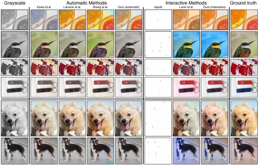
We show example results from our study in Figures 4 and 5. We compare the annotations to the seminal method proposed by Levin et al. (2004), along with the automatic output from our network. Qualitatively, the added user points typically add (1) saturation when the automatic result is lacking and (2) accurate higher frequency detail, that automatic methods have difficulty producing. Comparing our method to Levin et al. (2004), our method is more effective at finding segment boundaries given sparse user inputs. We do note that the user points are collected by running our system, which provides an advantage. However, collecting these points, with the right colors, is enabled by the interactive nature of our algorithm and our color recommendation system.

(a)

(b)

(c)

Figure 7. Unusual colorization (a) User inputs with unusual colors (b) Output colorization using user points with unusual colors (c) Output colorization with user points using conventional colors. Photograph by Corporal Michael Guinto, 2014 (Public Domain).

(a)

(b)

(c)

(d)

(e)

(f)

Figure 8. Multiple user colors within a segment. (a) Input grayscale image. (b,c) Output colorization conditioned on a single centered user point colored (b-blue, c-red). (d) Locations used for user points for (e) and (f). (e,f) Outputs given different user input colors (e-blue&red, f-green&pink).

Figure 9. Global histogram transfer Using our Global Hints Network, we colorize the grayscale version of the image on the left using global histograms from the top-right inset images. Images are from the Imagenet dataset (Russakovsky et al., 2015).

Figure 10. Legacy black and white photographs Our method applied to legacy black and white photographs. Top left: The Tetons and Snake River, Ansel Adams, 1942; Bottom left: Photo by John Rooney of Muhammad Ali versus Sonny Liston, 1965 (c.f. color photo by Neil Leifer at almost exactly the same moment); Right: V-J Day in Times Square, Alfred Eisenstaedt, 1945.

4.3. Does the network generalize to unusual colorizations?

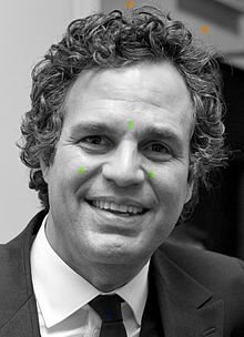
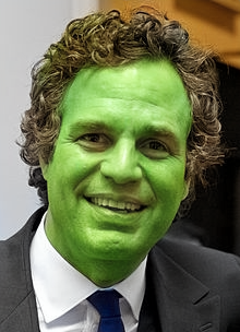
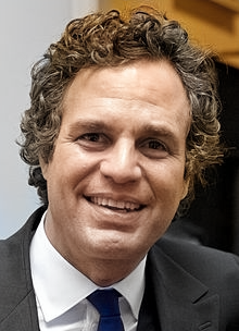
During training, we use natural images, and reveal the ground truth colors to simulate user input. However, there are use cases where the user may intentionally desire an unusual colorization. Will the network be able to follow the inputs in these cases? In Figure 7, we show an unusual colorization guided by the user, giving the actor a green face with three user points on the face. These results suggest that in the absence of nearby user inputs, the network will attempt to find an appropriate colorization for the object, based on the training corpus. However, once an input is provided by the user, the system fills in the segment with the desired color.

4.4. Is the system able to incorporate global statistics?

We train a variant of our system, taking global statistics as inputs, instead of local points. As described in Table 1, when given the ground truth statistics, such as the global histogram of colors or average saturation, the network achieves a higher PSNR scores, 27.9 and 25.6, respectively, than when performing automatic colorization (24.4), indicating that the network has learned how to fuse global statistics. We also test on the SUN-6 dataset, shown in Table 3, proposed by Deshpande et al. (2015). We show higher performance than Despande et al. (2015) and almost equal performance with Larsson et al. (2016), which fuses the predictions from an automatic colorization network with a ground truth histogram using an energy minimization procedure.

The network has only been trained on images with its own ground truth histogram. In Figure 9, we qualitatively the network’s generalization ability by computing the global histogram on separate reference images, and apply them to a photograph. The bird is an interesting test case, as it can be plausibly colorized in many different ways. We observe that that the color distributions of the reference input image is successfully transferred to the target grayscale image. Furthermore, the colorizations are realistic and diverse.

Method	Added Inputs	PSNR (dB)
Deshpande et al. (2015)	automatic	23.18 $\pm$ 0.20
Larsson et al. (2016)	automatic	25.60 $\pm$ 0.23
Ours	automatic	25.65 $\pm$ 0.23
Deshpande et al. (2015)	+ global hist	23.85 $\pm$ 0.23
Larsson et al. (2016)	+ global hist	28.62 $\pm$ 0.23
Ours	+ global hist	28.57 $\pm$ 0.21

Table 3. Global Histogram We test our Global Hints Network at incorporating the global truth histogram on 240 images from SUN used by (Deshpande et al., 2015).

4.5. How does the system respond to multiple colors within an equiluminant segment?

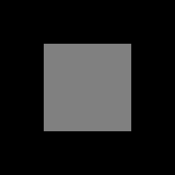
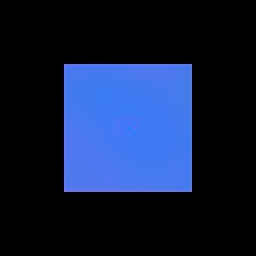
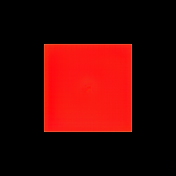
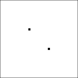
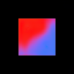
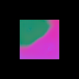
In natural images, chrominance changes almost never appear without a lightness change. In Figure 8(a), we show a toy example of an image of a gray square on top of a black square. If given a $7\times 7$ point in the center of the image, the system will successfully propagate the color to the center region, as shown in Figures 8(a)(b). However, how does the system respond if given two different colors within the same segment, as shown in Figure 8(d)? Given blue and red points, the system draws a seam between the two colors, as shown in Figure 8(e), where two points are placed symmetrically around the center of the image. Because our system is learned from data, it is difficult to characterize how the system will exactly behave in such a scenario. Qualitatively, we observe that the seam is not straight, and the shape as well as the sharpness of the transition is dependent on the colors. For example, in Figure 8(f), green and pink points produce a harder seam. We found similar behavior under similar scenarios in natural images as well.

4.6. Is the system able to colorize legacy photographs?

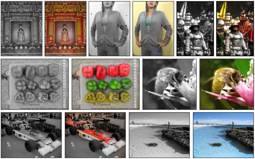
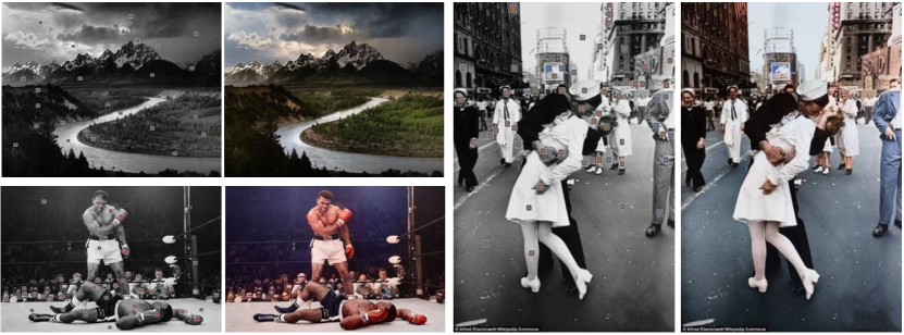
Our system was trained on “synthetic” grayscale images by removing the chrominance channels from color images. We qualitatively test our system on legacy grayscale images, and show some selected results in Figure 10.

5. Limitations and Discussion

A benefit of our system is that the network predicts user-intended actions based on learned semantic similarities. However, the network can also be over-optimistic and produce undesired non-local effects. For example, points added on a foreground object may cause an undesired change in the background, as shown on the last row in Figure 4. Qualitatively, we found that adding some control points can remedy this. In addition, the network can also fail to completely propagate a user point, as shown in the fifth row in Figure 4. In these instances, the user can fill in the region with additional input.

For scenes with difficult segmentation boundaries, the user sometimes needs to define boundaries explicitly by densely marking either side. Our system can continuously incorporate this information, even with hundreds of input points, as shown on Figure 6. Points can be added to fix color bleeding artifacts when the system has poor underlying segmentation. However, our interface is mainly designed for the “few seconds to couple minutes” interaction regime. For users wanting high-precision control and willing to spend hours per photograph, working in Photoshop is likely a better solution.

Our system is currently trained on points; we find that in this regime random sampling covers the low-dimensional workspace surprisingly well. However, a future step is to better simulate the user, and to effectively incorporate stroke-based inputs that traditional methods utilize. Integration between the local user points and global statistics inputs would be an interesting next step. Our interface code and models are publicly available at https://richzhang.github.io/ideepcolor, along with all images generated from the user study and random global histogram transfer results.

Change Log

v1 Initial release. SIGGRAPH camera ready version. DOI: http://dx.doi.org/10.1145/3072959.3073703

References

- (1)
- An and Pellacini (2008) Xiaobo An and Fabio Pellacini. 2008. AppProp: all-pairs appearance-space edit propagation. 27, 3 (2008), 40.
- Barnes et al. (2009) Connelly Barnes, Eli Shechtman, Adam Finkelstein, and Dan Goldman. 2009. PatchMatch: a randomized correspondence algorithm for structural image editing. ACM Transactions on Graphics (TOG) 28, 3 (2009), 24.
- Barron and Poole (2016) Jonathan T Barron and Ben Poole. 2016. The Fast Bilateral Solver. ECCV (2016).
- Bell et al. (2015) Sean Bell, Paul Upchurch, Noah Snavely, and Kavita Bala. 2015. Material recognition in the wild with the materials in context database. In CVPR. 3479–3487.
- Chang et al. (2015) Huiwen Chang, Ohad Fried, Yiming Liu, Stephen DiVerdi, and Adam Finkelstein. 2015. Palette-based photo recoloring. ACM Transactions on Graphics (TOG) 34, 4 (2015), 139.
- Charpiat et al. (2008) Guillaume Charpiat, Matthias Hofmann, and Bernhard Schölkopf. 2008. Automatic image colorization via multimodal predictions. In ECCV.
- Chen et al. (2012) Xiaowu Chen, Dongqing Zou, Qinping Zhao, and Ping Tan. 2012. Manifold preserving edit propagation. ACM Transactions on Graphics (TOG) 31, 6 (2012), 132.
- Cheng and Vishwanathan (2007) Li Cheng and SVN Vishwanathan. 2007. Learning to compress images and videos. In Proceedings of the 24th international conference on Machine learning. ACM, 161–168.
- Cheng et al. (2015) Zezhou Cheng, Qingxiong Yang, and Bin Sheng. 2015. Deep Colorization. In ICCV. 415–423.
- Chia et al. (2011) Alex Yong-Sang Chia, Shaojie Zhuo, Raj Kumar Gupta, Yu-Wing Tai, Siu-Yeung Cho, Ping Tan, and Stephen Lin. 2011. Semantic colorization with internet images. In ACM Transactions on Graphics (TOG), Vol. 30. ACM, 156.
- Deshpande et al. (2015) Aditya Deshpande, Jason Rock, and David Forsyth. 2015. Learning Large-Scale Automatic Image Colorization. In ICCV. 567–575.
- Endo et al. (2016) Yuki Endo, Satoshi Iizuka, Yoshihiro Kanamori, and Jun Mitani. 2016. DeepProp: Extracting Deep Features from a Single Image for Edit Propagation. In Computer Graphics Forum, Vol. 35. Wiley Online Library, 189–201.
- Frans (2017) Kevin Frans. 2017. Outline Colorization through Tandem Adversarial Networks. In arXiv:1704.08834.
- Gatys et al. (2016) Leon A Gatys, Alexander S Ecker, and Matthias Bethge. 2016. Image style transfer using convolutional neural networks. In CVPR. 2414–2423.
- Gharbi et al. (2016) Michaël Gharbi, Gaurav Chaurasia, Sylvain Paris, and Frédo Durand. 2016. Deep joint demosaicking and denoising. ACM Transactions on Graphics (TOG) 35, 6 (2016), 191.
- Girshick et al. (2014) Ross Girshick, Jeff Donahue, Trevor Darrell, and Jitendra Malik. 2014. Rich feature hierarchies for accurate object detection and semantic segmentation. In CVPR.
- Goodfellow et al. (2014) Ian Goodfellow, Jean Pouget-Abadie, Mehdi Mirza, Bing Xu, David Warde-Farley, Sherjil Ozair, Aaron Courville, and Yoshua Bengio. 2014. Generative adversarial nets. In NIPS. 2672–2680.
- Gupta et al. (2012) Raj Kumar Gupta, Alex Yong-Sang Chia, Deepu Rajan, Ee Sin Ng, and Huang Zhiyong. 2012. Image colorization using similar images. In Proceedings of the 20th ACM international conference on Multimedia. ACM, 369–378.
- Hariharan et al. (2015) Bharath Hariharan, Pablo Arbeláez, Ross Girshick, and Jitendra Malik. 2015. Hypercolumns for object segmentation and fine-grained localization. In CVPR. 447–456.
- He et al. (2009) Xiaofei He, Ming Ji, and Hujun Bao. 2009. A unified active and semi-supervised learning framework for image compression. In CVPR. IEEE, 65–72.
- Hertzmann et al. (2001) Aaron Hertzmann, Charles E Jacobs, Nuria Oliver, Brian Curless, and David H Salesin. 2001. Image analogies. In Proceedings of the 28th annual conference on Computer graphics and interactive techniques. ACM.
- Huang et al. (2005) Yi-Chin Huang, Yi-Shin Tung, Jun-Cheng Chen, Sung-Wen Wang, and Ja-Ling Wu. 2005. An adaptive edge detection based colorization algorithm and its applications. In Proceedings of the 13th annual ACM international conference on Multimedia. ACM, 351–354.
- Huber (1964) Peter J Huber. 1964. Robust estimation of a location parameter. The Annals of Mathematical Statistics 35, 1 (1964), 73–101.
- Iizuka et al. (2016) Satoshi Iizuka, Edgar Simo-Serra, and Hiroshi Ishikawa. 2016. Let there be Color!: Joint End-to-end Learning of Global and Local Image Priors for Automatic Image Colorization with Simultaneous Classification. SIGGRAPH 35, 4 (2016).
- Inc (2017) Preferred Networks Inc. 2017. Paints Chainer. (2017). https://github.com/pfnet/PaintsChainer
- Irony et al. (2005) Revital Irony, Daniel Cohen-Or, and Dani Lischinski. 2005. Colorization by example. In Eurographics Symp. on Rendering, Vol. 2. Citeseer.
- Isola et al. (2017) Phillip Isola, Jun-Yan Zhu, Tinghui Zhou, and Alexei A Efros. 2017. Image-to-image translation with conditional adversarial networks. CVPR (2017).
- Krizhevsky et al. (2012) Alex Krizhevsky, Ilya Sutskever, and Geoffrey E Hinton. 2012. Imagenet classification with deep convolutional neural networks. In NIPS. 1097–1105.
- Larsson et al. (2016) Gustav Larsson, Michael Maire, and Gregory Shakhnarovich. 2016. Learning Representations for Automatic Colorization. In ECCV.
- LeCun et al. (1998) Yann LeCun, Léon Bottou, Yoshua Bengio, and Patrick Haffner. 1998. Gradient-based learning applied to document recognition. Proc. IEEE 86, 11 (1998), 2278–2324.
- Levin et al. (2004) Anat Levin, Dani Lischinski, and Yair Weiss. 2004. Colorization using optimization. In ACM Transactions on Graphics (TOG), Vol. 23. ACM, 689–694.
- Li et al. (2015) Xujie Li, Hanli Zhao, Guizhi Nie, and Hui Huang. 2015. Image recoloring using geodesic distance based color harmonization. Computational Visual Media 1, 2 (2015), 143–155.
- Li et al. (2008) Yuanzhen Li, Edward Adelson, and Aseem Agarwala. 2008. ScribbleBoost: Adding Classification to Edge-Aware Interpolation of Local Image and Video Adjustments. In Computer Graphics Forum, Vol. 27. Wiley Online Library, 1255–1264.
- Liu et al. (2008) Xiaopei Liu, Liang Wan, Yingge Qu, Tien-Tsin Wong, Stephen Lin, Chi-Sing Leung, and Pheng-Ann Heng. 2008. Intrinsic colorization. In ACM Transactions on Graphics (TOG), Vol. 27. ACM, 152.
- Liu et al. (2014) Yiming Liu, Michael Cohen, Matt Uyttendaele, and Szymon Rusinkiewicz. 2014. AutoStyle: automatic style transfer from image collections to users’ images. In Computer Graphics Forum, Vol. 33. Wiley Online Library, 21–31.
- Luan et al. (2007) Qing Luan, Fang Wen, Daniel Cohen-Or, Lin Liang, Ying-Qing Xu, and Heung-Yeung Shum. 2007. Natural image colorization. In Proceedings of the 18th Eurographics conference on Rendering Techniques. Eurographics Association, 309–320.
- Morimoto et al. (2009) Yuji Morimoto, Yuichi Taguchi, and Takeshi Naemura. 2009. Automatic colorization of grayscale images using multiple images on the web. In SIGGRAPH’09: Posters. ACM, 32.
- Pathak et al. (2016) Deepak Pathak, Philipp Krähenbühl, Jeff Donahue, Trevor Darrell, and Alexei Efros. 2016. Context Encoders: Feature Learning by Inpainting. In CVPR.
- Qu et al. (2006) Yingge Qu, Tien-Tsin Wong, and Pheng-Ann Heng. 2006. Manga colorization. In ACM Transactions on Graphics (TOG), Vol. 25. ACM, 1214–1220.
- Reinhard et al. (2001) Erik Reinhard, Michael Ashikhmin, Bruce Gooch, and Peter Shirley. 2001. Color Transfer Between Images. IEEE Comput. Graph. Appl. 21, 5 (Sept. 2001), 34–41. DOI:http://dx.doi.org/10.1109/38.946629
- Ronneberger et al. (2015) Olaf Ronneberger, Philipp Fischer, and Thomas Brox. 2015. U-net: Convolutional networks for biomedical image segmentation. In International Conference on Medical Image Computing and Computer-Assisted Intervention. Springer, 234–241.
- Russakovsky et al. (2015) Olga Russakovsky, Jia Deng, Hao Su, Jonathan Krause, Sanjeev Satheesh, Sean Ma, Zhiheng Huang, Andrej Karpathy, Aditya Khosla, Michael Bernstein, and others. 2015. Imagenet large scale visual recognition challenge. IJCV 115, 3 (2015).
- Sangkloy et al. (2017) Patsorn Sangkloy, Jingwan Lu, Chen Fang, Fisher Yu, and James Hays. 2017. Scribbler: Controlling Deep Image Synthesis with Sketch and Color. CVPR (2017).
- Selim et al. (2016) Ahmed Selim, Mohamed Elgharib, and Linda Doyle. 2016. Painting style transfer for head portraits using convolutional neural networks. ACM Transactions on Graphics (TOG) 35, 4 (2016), 129.
- Simo-Serra et al. (2016) Edgar Simo-Serra, Satoshi Iizuka, Kazuma Sasaki, and Hiroshi Ishikawa. 2016. Learning to simplify: fully convolutional networks for rough sketch cleanup. ACM Transactions on Graphics (TOG) 35, 4 (2016), 121.
- Simonyan and Zisserman (2014) Karen Simonyan and Andrew Zisserman. 2014. Very deep convolutional networks for large-scale image recognition. arXiv preprint arXiv:1409.1556 (2014).
- Wang et al. (2010) Baoyuan Wang, Yizhou Yu, Tien-Tsin Wong, Chun Chen, and Ying-Qing Xu. 2010. Data-driven image color theme enhancement. In ACM Transactions on Graphics (TOG), Vol. 29. ACM, 146.
- Wang et al. (2016) Ting-Chun Wang, Jun-Yan Zhu, Ebi Hiroaki, Manmohan Chandraker, Alexei A Efros, and Ravi Ramamoorthi. 2016. A 4D light-field dataset and CNN architectures for material recognition. In ECCV. Springer, 121–138.
- Welsh et al. (2002) Tomihisa Welsh, Michael Ashikhmin, and Klaus Mueller. 2002. Transferring color to greyscale images. ACM Transactions on Graphics (TOG) 21, 3 (2002), 277–280.
- Xie and Tu (2015) Saining Xie and Zhuowen Tu. 2015. Holistically-nested edge detection. In ICCV.
- Xu et al. (2009) Kun Xu, Yong Li, Tao Ju, Shi-Min Hu, and Tian-Qiang Liu. 2009. Efficient affinity-based edit propagation using kd tree. ACM Transactions on Graphics (TOG) 28, 5 (2009), 118.
- Xu et al. (2013) Li Xu, Qiong Yan, and Jiaya Jia. 2013. A sparse control model for image and video editing. ACM Transactions on Graphics (TOG) 32, 6 (2013), 197.
- Xu et al. (2016) Ning Xu, Brian Price, Scott Cohen, Jimei Yang, and Thomas S Huang. 2016. Deep interactive object selection. In CVPR.
- Yan et al. (2016) Zhicheng Yan, Hao Zhang, Baoyuan Wang, Sylvain Paris, and Yizhou Yu. 2016. Automatic photo adjustment using deep neural networks. ACM Transactions on Graphics (TOG) 35, 2 (2016), 11.
- Yu and Koltun (2016) Fisher Yu and Vladlen Koltun. 2016. Multi-Scale Context Aggregation by Dilated Convolutions. International Conference on Learning Representations (2016).
- Zhang et al. (2016) Richard Zhang, Phillip Isola, and Alexei A Efros. 2016. Colorful Image Colorization. In ECCV.
- Zhou et al. (2014) Bolei Zhou, Agata Lapedriza, Jianxiong Xiao, Antonio Torralba, and Aude Oliva. 2014. Learning deep features for scene recognition using places database. In NIPS.
- Zhu et al. (2015) Jun-Yan Zhu, Philipp Krahenbuhl, Eli Shechtman, and Alexei A Efros. 2015. Learning a discriminative model for the perception of realism in composite images. In CVPR.
- Zhu et al. (2016) Jun-Yan Zhu, Philipp Krähenbühl, Eli Shechtman, and Alexei A Efros. 2016. Generative visual manipulation on the natural image manifold. (2016).